A microscopic instability in neutral magnetized plasmas

Abstract

We show that in a neutral magnetized plasma there exist microscopic oscillatory modes, with wavelengths of the order of magnitude of the mean interparticle distance, which become unstable when the electron density exceeds a limit proportional to the square of the magnetic field. The model we consider is just a linearization of the classical one for neutral plasmas, namely a system of electrons subjected to Coulomb interactions among themselves and with a uniform positive neutralizing background. This model is here dealt with as an actual many-body problem, without introducing any averaging over the individual particles. The expression of the density limit coincides, apart possibly from a numerical factor of order one, with the well-known Brillouin density limit for a nonneutral plasma, which has however a macroscopic origin. The density limit here found has the same order of magnitude as the operational density limit observed in several conventional tokamak devices. We finally show that, when the full electromagnetic interactions are taken into account, dispersion relations are obtained which for short wavelengths reduce to those obtained here in the purely Coulomb case, and for long wavelengths reproduce the familiar ones of MHD.

I Introduction

It is well known that the magnetic confinement of a pure electron plasma is possible only for electron densities $n_{e}$ below the so-called Brillouin density limit brill ; davidson given by

$$n_{e}^{M}=\eta^{M}\frac{\epsilon_{0}B^{2}}{m_{e}}\,,$$ (1)

where $\eta^{M}=1/2$, while $B$, $\epsilon_{0}$ and $m_{e}$ are the magnetic field, the permittivity of free space, and the electron mass. The condition $n_{e}<n_{e}^{M}$ can be equivalently expressed as $\eta<\eta^{M}$ in terms of the dimensionless parameter

$$\eta\equiv\frac{m_{e}n_{e}}{\epsilon_{0}B^{2}}=\frac{\omega_{p}^{2}}{\omega_{c}^{2}}\,,$$ (2)

where $\omega_{p}=e\sqrt{n_{e}/\epsilon_{0}m_{e}}$ and $\omega_{c}=Be/m_{e}$ are the electron plasma frequency and cyclotron frequency respectively, $-e$ being the electron charge. The Brillouin density limit for a nonneutral plasma is usually derived by studying under a mean-field approximation the motion of a single generic electron of the plasma: for densities beyond the limit, the electrostatic repulsion due to the other charges cannot be counterbalanced by the Lorentz confining force exerted by the magnetic field.

In the present paper we show that a density limit exactly of the form (1) — possibly with a slightly different value of the critical parameter $\eta^{M}$ — exists for neutral plasmas too, inasmuch as the plasma presents an internal dynamical instability beyond that limit. Here however the instability can be revealed only by dealing with a microscopic many-body model involving the mutual Coulomb interaction of the individual charges, because it mainly concerns modes of wavelength of the order of the interparticle distance.

The model we consider is just the classical one of point electrons obeying Newton’s equations in an external magnetic field, with Coulomb interactions both among themselves and with a smeared-out positive neutralizing background. Such a model is considered for example in the works of Bohm, Gross and Pines bg1 ; bp1 ; pb2 , and in the previous ones of Langmuir and Tonks langmuir ; tonks . In the impossibility of dealing with the general analytical solution for such a many-body problem, those authors introduced in the equations of motion some averaging with respect to the individual particle positions, and as a consequence were compelled to consider only plasma oscillations with wavelengths much longer than the mean interparticle distance. Since, on the contrary, we are interested in the study of modes with short wavelengths, we have to adopt a different approach. We thus choose to stick with the original many-body problem, and to retain in the description of the system the microscopic coordinates of all the individual electrons. In order to simplify the mathematical equations, we then perform a linearization about an equilibrium configuration of the system. As already pointed out in a classical paper by Langmuir langmuir , the equilibrium condition requires the electrons to lie on the sites of some regular lattice. It turns out that the normal mode solutions of the linearized equations can be studied analytically, leading to dispersion relations which depend parametrically on the plasma density. If one considers in particular oscillations about a simple cubic lattice it turns out that, for densities larger than a limit of the form (1), there exists a relevant fraction of modes for which the frequency becomes complex, and so the system becomes unstable. This instability concerns modes of wavelength of the order of the interparticle distance, and so cannot be revealed by the methods of Bohm, Gross and Pines, or by the equations of magnetohydrodynamics (MHD).

The essential microscopic nature of the phenomenon discussed here also emerges from considerations of an energetic type. The origin of the instability lies in the fact that the equilibrium configuration here considered is not a minimum of the potential energy of the system. Indeed, it will be shown that the potential energy decreases for global displacements involving all the electrons of the system, when such displacements are described by plane waves with wavevectors having certain directions. In the absence of a magnetic field, the normal modes associated with such wavevectors are thus unstable. For a fixed density, an external magnetic field of large enough magnitude can stabilize them, but below a critical value the modes of shortest wavelengths along those directions become unstable.

We will also briefly discuss the possible significance of this instability in connection with the density limit empirically encountered in the operation of tokamaks for fusion research on magnetic confinement, pointing out that in several cases the density limit found here is of the same order of magnitude as the experimental one.

The equations of motion and their linearization are given in section II, together with the equation for the normal modes and the corresponding expression of the energy. In section III the form of the dispersion relations is studied in dependence of the relevant parameter $\eta=\omega_{p}^{2}/\omega_{c}^{2}$, and the existence of the instability is exhibited. In section IV a generalization of the model is considered, in which the full electromagnetic interactions are introduced, including retardation and radiative terms. We prove that the purely Coulomb model considered in the previous sections is recovered for short wavelengths, while in the long wavelength limit the dispersion relations exactly coincide with those provided by the macroscopic equations of MHD for a low temperature plasma. Finally, the possible physical relevance of the instability discussed here is briefly addressed in the Conclusion.

Three appendices are devoted to the technical details of some calculations. They concern respectively the effective field acting on an electron inside the plasma, the electrostatic energy in the equilibrium configuration of the plasma, and the dependence of the instability threshold on the orientation of the magnetic field.

II The model

II.1 The equations of motion and their linearization

Denoting by $\mathbf{z}_{i}$ the position vector of the $i$-th electron, its equation of motion is

$$m_{e}\ddot{\mathbf{z}}_{i}=-e{\mathbf{e}}_{i}({\mathbf{z}}_{i},t)-e\dot{\mathbf{z}}_{i}\times{\mathbf{B}}\,,$$ (3)

where ${\mathbf{e}}_{i}$ is the Coulomb field generated by all the other electrons and by the positive background, and ${\mathbf{B}}$ is an external magnetic field, which is supposed to be constant.

In order to obtain a linearized system of equations of motion, we look for an equilibrium configuration for the electrons. If the plasma is assumed to be infinite (i.e., if all edge effects are neglected), it is easy to see that such an equilibrium configuration is given by the points of any arbitrary simple Bravais lattice. Naming ${\bf a}_{1}$, ${\bf a}_{2}$, ${\bf a}_{3}$ the primitive translation vectors of the lattice, we have $n_{e}=1/V$, where $V=|{\bf a}_{1}\cdot{\bf a}_{2}\times{\bf a}_{3}|$ is the volume of the primitive cell, so that $a=V^{1/3}$ represents the lattice parameter. We denote by ${\bf r}_{{\bf n}}=n_{1}{\bf a}_{1}+n_{2}{\bf a}_{2}+n_{3}{\bf a}_{3}$ the position vector of an arbitrary point of the lattice, labelled by the triple of relative integers $\mathbf{n}=(n_{1},n_{2},n_{3})\in\mathbf{Z}^{3}$. We shall also label with ${\mathbf{n}}$ the electron associated with this lattice site, and so we denote by ${\mathbf{z}}_{\mathbf{n}}$ its position vector. Finally, we introduce the corresponding displacement ${\mathbf{x}}_{\mathbf{n}}$ by

$${\mathbf{z}}_{\mathbf{n}}(t)={\mathbf{r}}_{\mathbf{n}}+{\mathbf{x}}_{\mathbf{n}}(t)\,.$$

The linearized equations of motion about the chosen equilibrium configuration of the system can be shown, for all $\mathbf{n}\in\mathbf{Z}^{3}$, to be

$$m_{e}\ddot{\mathbf{x}}_{\mathbf{n}}=-\frac{n_{e}e^{2}}{3\epsilon_{0}}{\mathbf{x}}_{\mathbf{n}}-e\dot{\mathbf{x}}_{\mathbf{n}}\times{\mathbf{B}}+\frac{e^{2}}{4\pi\epsilon_{0}}\sum_{{\mathbf{m}}\neq{\mathbf{n}}}\widehat{\mathbf{D}}_{\mathbf{n}-\mathbf{m}}\cdot\mathbf{x}_{\mathbf{m}}\,,$$ (4)

where $\widehat{\mathbf{D}}_{\mathbf{m}}$, for $\mathbf{m}\in\mathbf{Z}^{3}$, $\mathbf{m}\neq\mathbf{0}$, is a symmetric matrix whose elements depend on the lattice geometry, namely

$$(\widehat{\mathbf{D}}_{\mathbf{m}})_{ij}=\bigg{[}3\frac{({\mathbf{r}}_{\mathbf{m}})_{i}({\mathbf{r}}_{\mathbf{m}})_{j}}{|{\mathbf{r}}_{\mathbf{m}}|^{5}}-\frac{\delta_{ij}}{|{\mathbf{r}}_{\mathbf{m}}|^{3}}\bigg{]}\,.$$ (5)

In order to prove (4), let us start from the general equation (3), and observe that up to first order in the displacements ${\mathbf{x}}_{\mathbf{m}}$ of the electrons one can write

$${\mathbf{e}}_{\mathbf{n}}({\mathbf{z}}_{\mathbf{n}},t)={\mathbf{e}}_{\mathbf{n}}^{(0)}({\mathbf{z}}_{\mathbf{n}})+{\mathbf{e}}_{\mathbf{n}}^{(1)}({\mathbf{r}}_{\mathbf{n}},t)\,,$$

where ${\mathbf{e}}_{\mathbf{n}}^{(0)}$ and ${\mathbf{e}}_{\mathbf{n}}^{(1)}$ are respectively the contributions to the field ${\mathbf{e}}_{\mathbf{n}}$ of order zero and one in the ${\mathbf{x}}_{\mathbf{m}}$.

It is clear that ${\mathbf{e}}^{(0)}_{\mathbf{n}}$ is given by the constant electrostatic field generated by the background and by the electrons ${\mathbf{m}}\neq{\mathbf{n}}$, when all these electrons are kept fixed at their equilibrium positions. Since the Bravais lattice is invariant under spatial reflections, we have ${\mathbf{e}}^{(0)}_{\mathbf{n}}({\mathbf{r}}_{\mathbf{n}})=0$. This is actually the reason why, as we said before, the points of the lattice are equilibrium positions for the electrons. Moreover, since the plasma is assumed to be globally neutral, the charge density of the background must be $\rho_{\rm bg}=n_{e}e$. From $\textrm{div}\,{\mathbf{e}}^{(0)}_{\mathbf{n}}({\mathbf{r}}_{\mathbf{n}})=\rho_{\rm bg}/\epsilon_{0}=n_{e}e/\epsilon_{0}$, assuming that the lattice is isotropic it then follows that $\partial({\mathbf{e}}^{(0)}_{\mathbf{n}})_{i}/\partial x_{j}({\mathbf{r}}_{\mathbf{n}})=\delta_{ij}n_{e}e/3\epsilon_{0}$. Hence, to first order in ${\mathbf{x}}_{\mathbf{n}}$ we can write

$${\mathbf{e}}^{(0)}_{\mathbf{n}}({\mathbf{z}}_{\mathbf{n}})=\frac{n_{e}e}{3\epsilon_{0}}{\mathbf{x}}_{\mathbf{n}}\,.$$ (6)

Concerning ${\mathbf{e}}_{\mathbf{n}}^{(1)}$, it is given by the sum of the Coulomb fields generated by all the electrons ${\mathbf{m}}\neq{\mathbf{n}}$, computed at order one in their displacements ${\mathbf{x}}_{\mathbf{m}}$. Such contributions are given by the well-known expression (see for instance chapter 4 of ref. Jackson ) of the field $\mathbf{E}_{\mathbf{m}}$ generated by an electric dipole $-e{\mathbf{x}}_{\mathbf{m}}$ located at $\mathbf{r}_{\mathbf{m}}$, that is

$$\mathbf{E}_{\mathbf{m}}(\mathbf{x})=-\frac{e}{4\pi\epsilon_{0}}\left(3\frac{\mathbf{x}_{\mathbf{m}}\cdot\mathbf{y}}{y^{5}}\mathbf{y}-\frac{\mathbf{x}_{\mathbf{m}}}{y^{3}}\right)\,,$$ (7)

with $\mathbf{y}=\mathbf{x}-\mathbf{r}_{\mathbf{m}}$. It follows that

$${\mathbf{e}}_{\mathbf{n}}^{(1)}({\mathbf{r}}_{\mathbf{n}},t)=\sum_{{\mathbf{m}}\neq{\mathbf{n}}}\mathbf{E}_{\mathbf{m}}(\mathbf{r}_{\mathbf{n}})=-\frac{e}{4\pi\epsilon_{0}}\sum_{{\mathbf{m}}\neq{\mathbf{n}}}\widehat{\mathbf{D}}_{\mathbf{n}-\mathbf{m}}\cdot\mathbf{x}_{\mathbf{m}}\,,$$ (8)

with $\widehat{\mathbf{D}}$ given by (5). From (6) and (8), equation (4) is then readily obtained.

II.2 The equation for the normal modes

In order to deal with the infinite system of linear differential equations (4), we shall look as usual for normal mode solutions of the form

$${\mathbf{x}}_{{\mathbf{n}}}={\mathbf{C}}\exp\left[i({\mathbf{k}}\cdot{\bf r}_{{\bf n}}-\omega t)\right]\,,$$ (9)

where the wavevector ${\mathbf{k}}$, the frequency $\omega$ and the polarization vector ${\mathbf{C}}$ are constants. For such an ansatz, the field ${\mathbf{e}}_{\mathbf{n}}^{(1)}({\mathbf{r}}_{\mathbf{n}},t)$ becomes

$${\mathbf{e}}_{\mathbf{n}}^{(1)}({\mathbf{r}}_{\mathbf{n}},t)=-\frac{en_{e}}{\epsilon_{0}}\widehat{\mathbf{M}}({\mathbf{q}})\cdot\mathbf{C}\exp[i(\mathbf{k}\cdot\mathbf{r}_{\mathbf{n}}-\omega t)]\,,$$ (10)

where we have introduced the real dimensionless symmetric matrix

$$\widehat{\mathbf{M}}({\mathbf{q}})=\frac{V}{4\pi}\sum_{{\mathbf{m}}\neq{\mathbf{0}}}\widehat{\mathbf{D}}_{\mathbf{m}}\exp(2\pi i\mathbf{q}\cdot\mathbf{r}_{\mathbf{m}}/a)\,,$$ (11)

which depends on the wavevector $\mathbf{k}$ and on the lattice parameter $a$ only through their product

$$\mathbf{q}\equiv\mathbf{k}a/2\pi\,.$$

Note that the series in (11) converges only in an improper sense. In appendix A, using techniques analogous to those already developed in mcg , we obtain an expression for $\widehat{\mathbf{M}}({\mathbf{q}})$ given by the sum of an absolutely convergent series. For an isotropic lattice, this expression can be written as

$$M_{ij}({\mathbf{q}})=\frac{\delta_{ij}}{3}-\frac{q_{i}q_{j}}{{\mathbf{q}}^{2}}+N_{ij}({\mathbf{q}})\,,$$ (12)

with

$$N_{ij}({\mathbf{q}})=\ (\alpha/3-2\beta){\bf q}^{2}\delta_{ij}+(\alpha-4\beta)q_{i}q_{j}$$

$$+2(5\beta-\alpha)q_{i}^{2}\delta_{ij}-\sum_{\mathbf{m}\neq 0}\bar{c}_{ij}(\mathbf{H}_{\mathbf{m}},\mathbf{q})\,.$$ (13)

Here the sum runs over all the points of the dimensionless reciprocal lattice with $\mathbf{m}\neq 0$, namely

$$\mathbf{H}_{\mathbf{m}}\equiv\frac{1}{a^{2}}(m_{1}\mathbf{a}_{2}\times\mathbf{a}_{3}+m_{2}\mathbf{a}_{3}\times\mathbf{a}_{1}+m_{3}\mathbf{a}_{1}\times\mathbf{a}_{2})\,,$$ (14)

and the function $\bar{c}_{ij}$ is obtained by subtracting to the function

$$c_{ij}(\mathbf{H},\mathbf{q})=\frac{(H_{i}+q_{i})(H_{j}+q_{j})}{({\bf H}+{\bf q})^{2}}$$ (15)

the terms of order $k\leq 3$ of its Taylor expansion in the variable $\mathbf{q}/H$ about the origin. Finally, the constants $\alpha$ and $\beta$ can be numerically computed for any given geometry of the lattice using formulas (40)–(41). Note that ${\rm Tr}\,\widehat{\mathbf{N}}(\mathbf{q})=0$ for all $\mathbf{q}$.

The term $\delta_{ij}/3$ on the right-hand side of (12) is the equivalent of the so-called “Lorentz term” in the expression of the local field inside isotropic dielectrics. Its contribution to the equation of motion exactly cancels the first term on the right-hand side of (4).

In conclusion, the normal mode ansatz (9) for the linearized equation of motion (4) leads to a linear equation for the polarization vector $\mathbf{C}$, namely

$$i\frac{\omega e}{m_{e}}\mathbf{B}\times\mathbf{C}-\omega^{2}\mathbf{C}=\omega_{p}^{2}\left[-\frac{\mathbf{q}}{\mathbf{q}^{2}}\mathbf{q}\cdot\mathbf{C}+\widehat{\mathbf{N}}({\mathbf{q}})\cdot\mathbf{C}\right]\,,$$ (16)

where $\omega_{p}=e\sqrt{n_{e}/\epsilon_{0}m_{e}}$ is the electron plasma frequency. This is an equation of the form $\widehat{\mathbf{A}}\cdot\mathbf{C}=0$, with the matrix $\widehat{\mathbf{A}}$ given by

$$A_{ij}(\mathbf{q},\omega)=\ i\frac{\omega e}{m_{e}}\epsilon_{ijk}B_{k}+\omega^{2}\delta_{ij}-\omega_{p}^{2}\left[\frac{q_{i}q_{j}}{q^{2}}-N_{ij}({\mathbf{q}})\right]\,,$$ (17)

where $\epsilon_{ijk}$ denotes the completely antisymmetric tensor such that $\epsilon_{123}=1$. The condition for the existence of nontrivial solutions is ${\rm det}\,\widehat{\mathbf{A}}(\mathbf{q},\omega)=0$. By solving this last equation with respect to $\omega$ for a given $\mathbf{q}$, one obtains the dispersion relation for the oscillations in our model of magnetized plasma.

II.3 The energy

As the normal modes discussed here have a purely electrostatic nature, it is of interest to have available an analytical expression for the electrostatic energy $U$ of the system. It is easy to see that

$$U=-\frac{e}{2}\sum_{\mathbf{n}}\phi_{\mathbf{n}}(\mathbf{z}_{\mathbf{n}})\,,$$ (18)

where $\phi_{\mathbf{n}}$ is the electrostatic potential generated by all the charges of the plasma (electrons and background) except the electron $\mathbf{n}$. The energy $U_{0}$, corresponding to the configuration in which all the electrons are at their equilibrium positions, i.e. $\mathbf{z}_{\mathbf{n}}=\mathbf{r}_{\mathbf{n}}$ for all $\mathbf{n}\in\mathbf{Z}^{3}$, can be evaluated by means of a suitable modification of the Ewald method for the calculation of the electrostatic energy of a ionic lattice (see for instance appendix B of kittel ). If $N$ is the total number of electrons in the plasma, which is assumed to be so big that the surface effects can be neglected, we have

$$U_{0}=-N\frac{be^{2}}{8\pi\epsilon_{0}a}\,,$$ (19)

where the dimensionless constant $b$ can be calculated using the formula

$$b= -\sum_{\mathbf{m}\neq\mathbf{0}}\frac{\exp(-\pi\mathbf{H}_{\mathbf{m}}^{2}/\xi)}{\pi\mathbf{H}_{\mathbf{m}}^{2}}-\sum_{\mathbf{n}\neq\mathbf{0}}\frac{F(\sqrt{\pi\xi}|\mathbf{r}_{\mathbf{n}}|/a)}{|\mathbf{r}_{\mathbf{n}}|/a}$$

$$+\frac{1}{\xi}+2\sqrt{\xi}\,,$$ (20)

involving a positive parameter $\xi$. In this formula the function $F$ is defined as

$$F(x)=\frac{2}{\pi}\int_{x}^{+\infty}e^{-s^{2}}ds\,.$$ (21)

It can be proved that the right-hand side of (II.3) is independent of the value of $\xi$, and that both sums converge very quickly for $\xi$ of order unity. The calculations leading to (II.3) are carried out in appendix B.

Since ${\mathbf{e}}_{\mathbf{n}}({\mathbf{z}}_{\mathbf{n}},t)=-{\mathbf{\nabla}}\phi_{\mathbf{n}}(\mathbf{z}_{\mathbf{n}})$, it follows from (6) and (8) that up to second order in the displacements $\mathbf{x}_{\mathbf{n}}$ we have

$$U=U_{0}+\frac{n_{e}e^{2}}{6\epsilon_{0}}\sum_{\mathbf{n}}{\mathbf{x}}_{\mathbf{n}}^{2}-\frac{e^{2}}{8\pi\epsilon_{0}}\sum_{{\mathbf{m}}\neq{\mathbf{n}}}\mathbf{x}_{\mathbf{n}}\cdot\widehat{\mathbf{D}}_{\mathbf{n}-\mathbf{m}}\cdot\mathbf{x}_{\mathbf{m}}\,.$$ (22)

The total energy, which is conserved on the solutions of the equations of the motion, is then $E=T+U$, where $T=(m_{e}/2)\sum_{\mathbf{n}}\dot{\mathbf{x}}_{\mathbf{n}}^{2}$ is the kinetic energy.

For a normal mode of the form (9), it follows from (22) that the electrostatic energy per electron $U/N$ is given by

$$\frac{U}{N}= -\frac{be^{2}}{8\pi\epsilon_{0}a}+\frac{m_{e}\omega_{p}^{2}}{4}\mathbf{C}^{*}\cdot\left[\hat{\mathbf{1}}/3-\hat{\mathbf{M}}(\mathbf{q})\right]\cdot\mathbf{C}$$ (23)

$$= -\frac{be^{2}}{8\pi\epsilon_{0}a}+\frac{m_{e}\omega_{p}^{2}}{4}\left[\frac{|\mathbf{q}\cdot\mathbf{C}|^{2}}{\mathbf{q}^{2}}-\mathbf{C}^{*}\cdot\hat{\mathbf{N}}(\mathbf{q})\cdot\mathbf{C}\right]\,.$$

Then, for the total energy per electron $E/N$ of the normal mode we obtain

$$\frac{E}{N}= -\frac{be^{2}}{8\pi\epsilon_{0}a}+\frac{m_{e}\omega_{p}^{2}}{4}\mathbf{C}^{*}\cdot\left[\hat{\mathbf{1}}/3-\hat{\mathbf{M}}(\mathbf{q})\right]\cdot\mathbf{C}$$

$$+\frac{m_{e}\omega^{2}}{4}|\mathbf{C}|^{2}$$

$$= -\frac{be^{2}}{8\pi\epsilon_{0}a}+\frac{m_{e}\omega^{2}}{2}|\mathbf{C}|^{2}-i\frac{\omega e}{4}\mathbf{B}\cdot\mathbf{C}\times\mathbf{C}^{*}\,,$$

where the last equality follows from the equation of motion (16).

Equation (22) shows that the potential energy always increases when a single electron is displaced from its equilibrium position, all the others being kept fixed. We see however from (23) that, if for some $\mathbf{q}$ the matrix $\omega_{p}^{2}(\hat{\mathbf{1}}/3-\hat{\mathbf{M}}(\mathbf{q}))$ has a negative eigenvalue corresponding to some eigenvector $\mathbf{C}$, then the potential energy is decreased by a simultaneous displacement of all the electrons according to the pattern described by the polarization vector $\mathbf{C}$ and the wavevector $\mathbf{q}$. This means that, in such a case, the potential energy at the equilibrium configuration does not present a minimum. This is directly connected with the existence of unstable modes since, according to the dynamical equation (16), for $\mathbf{B}=0$ the squared frequency $\omega^{2}$ of the normal modes is just given by an eigenvalue of the matrix $\omega_{p}^{2}(\hat{\mathbf{1}}/3-\hat{\mathbf{M}}(\mathbf{q}))$. Hence negative eigenvalues give rise to imaginary values of the frequency. We will see in the next section that negative eigenvalues actually exist in the case of the simple cubic lattice, when $\mathbf{q}$ is parallel to one of the three principal axes.

III Unstable modes of oscillation

III.1 Dispersion relations and existence of unstable modes

To find the dispersion relations we have to solve the linear equation (16). This contains the function ${\mathbf{N}}({\mathbf{q}})$ given by (II.2), which depends on the particular geometry of the Bravais lattice. In the present paper we limit ourselves to considering the easiest possible case, namely that of a simple cubic lattice, for which the primitive translation vectors are parallel to the three basic unit vectors of a cartesian frame: $\mathbf{a}_{i}=a\mathbf{u}_{i}$, $i=1,2,3$. In this case the reciprocal lattice is also simple cubic, and we have from (14) $\mathbf{H}_{\mathbf{m}}=\mathbf{m}$, with ${\mathbf{m}}\in\mathbf{Z}^{3}$. For this lattice the geometrical constants appearing in (II.2) are $\alpha\cong 8.9136$ and $\beta\cong 1.2267$. Moreover, the constant $b$ appearing in the expression (19) of the electrostatic energy at equilibrium is $b\cong 2.8373$.

Let us consider the particular case in which the wavevector $\mathbf{k}$ is parallel to a principal lattice axis, say $\mathbf{u}_{3}$. In such a case the matrix ${\mathbf{N}}({\mathbf{q}})$ becomes diagonal. We shall denote $N_{11}(q{\mathbf{u}}_{3})=N_{22}(q{\mathbf{u}}_{3})\equiv\bar{N}(q)$, so that $N_{33}(q{\mathbf{u}}_{3})=-2\bar{N}(q)$. The graph of the function $\bar{N}(q)$ is displayed in Fig. 1. It is easily seen from (16) that the dispersion relations, when expressed in terms of the quantities $q$ and

$$\widetilde{\omega}\equiv\omega/\omega_{c}\,,$$

contain the single positive parameter $\eta=\omega_{p}^{2}/\omega_{c}^{2}$. For instance, if $\mathbf{B}$ is also parallel to $\mathbf{u}_{3}$, then the dispersion relation for transversal normal modes is implicitly expressed by the equation

$$\widetilde{\omega}^{2}-\widetilde{\omega}+\eta\bar{N}(q)=0\,.$$ (24)

For these modes, the electrons move along circular orbits in planes orthogonal to $\mathbf{B}$.

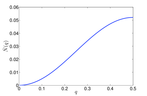
Figure 1: Graph of the function $\bar{N}(q)$.

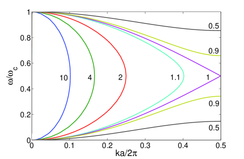
Figure 2: Dispersion curves for $\mathbf{k}$ and $\mathbf{B}$ both parallel to an axis of the simple cubic lattice, and circular transversal polarization. The number next to each curve gives the corresponding value of the ratio $\eta/\eta_{C}$, with $\eta=\omega_{p}^{2}/\omega_{c}^{2}$ and $\eta_{C}\cong 4.80$.

In Fig. 2 we plot the dispersion curves obtained from a numerical solution of (24) for various values of $\eta$. This is the figure in which the phenomenon of microscopic plasma instabilities manifests itself. We see in fact that the curves are defined in the whole Brillouin zone $0\leq q\leq 1/2$ only for $\eta$ below a certain critical value $\eta_{C}\cong 4.80$. This obviously follows from the fact that (24) is a second degree equation in $\widetilde{\omega}$, which admits two real solutions only for $\eta\leq 1/(4\bar{N}(q))$. For $\eta=\eta_{C}$ there exists a double real solution for $q=1/2$, hence

$$\eta_{C}=\frac{1}{4\bar{N}(1/2)}\cong 4.80\,.$$

If $\eta>\eta_{C}$, for $q$ sufficiently near to 1/2 (i.e. for sufficiently short wavelengths) the two solutions of (24) are complex conjugate. For one of these solutions the electrons simultaneously spiral away from their equilibrium positions, so that the normal mode becomes unstable.

Considering again the case in which both $\mathbf{k}$ and $\mathbf{B}$ are parallel to $\mathbf{u}_{3}$, from (16) we have for the longitudinal modes

$$\widetilde{\omega}^{2}=\eta\left(1+2\bar{N}(q)\right)\,.$$ (25)

Since the right-hand side of this equality is always positive, we see that for these modes $\omega$ is real for all $q$ and all $\eta$.

Let us now consider the case in which $\mathbf{k}$ is still parallel to $\mathbf{u}_{3}$, but $\mathbf{B}$ is parallel to $\mathbf{u}_{2}$. For the transversal mode with $\mathbf{C}$ parallel to $\mathbf{B}$ we find the relation $\omega^{2}=-\omega_{p}^{2}\bar{N}(q)$, or

$$\widetilde{\omega}^{2}=-\eta\bar{N}(q)\,.$$ (26)

The right-hand side is in this case always negative, hence this equation provides two opposite imaginary values for $\omega$. This means that, for all $\eta>0$, there exists an unstable mode for which the electrons move exponentially away from the equilibrium positions along the direction of $\mathbf{B}$. Furthermore, for elliptic orbits orthogonal to $\mathbf{B}$ we have

$$\widetilde{\omega}^{4}-\left[1+(1+\bar{N}(q))\eta\right]\widetilde{\omega}^{2}-\bar{N}(q)(1+2\bar{N}(q))\eta^{2}=0\,.$$ (27)

This second degree equation in $\widetilde{\omega}^{2}$ always admits two real solutions of opposite signs, hence there exist a stable and an unstable mode of this type for all $q$ and all $\eta>0$.

The dispersion curves for all the stable modes considered above, with $\mathbf{q}$ parallel to a lattice axis, are reported in the right part of Fig. 3 for the particular value $\eta=3$. The solid lines correspond to the cases in which $\mathbf{B}$ is parallel to $\mathbf{q}$. In particular, the two lower ones refer to transversal modes and are derived from (24). They can thus be compared with the curves of Fig. 2, noticing that $\eta=3$ corresponds to $\eta/\eta_{C}=0.625$. The top solid line refers instead to the longitudinal modes described by (25). Finally, the dashed line corresponds to the case in which $\mathbf{B}$ is orthogonal to $\mathbf{q}$, and is derived from (27).

The left part of Fig. 3 shows the behavior of the same curves in the long-wavelength limit, i.e. for $q\ll 1$, as resulting from the full electromagnetic treatment given in section IV. We will show that in this limit the dispersion relations derived from our model exactly coincide with those provided by the equations of MHD for a zero temperature plasma.

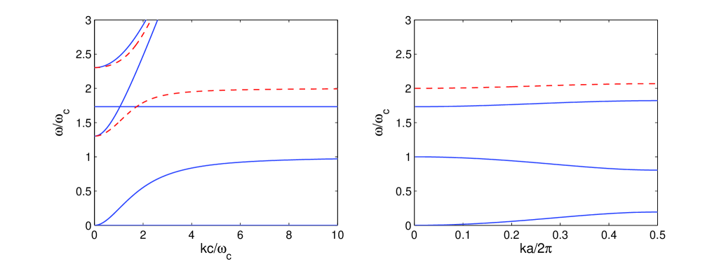
Figure 3: Dispersion curves obtained from our model for $\omega_{p}^{2}/\omega_{c}^{2}=3$, at two different scales of the $k$ axis. It is assumed that $\omega_{c}a/2\pi c\approx 10^{-5}$, so the left graph shows the behavior for $ka/2\pi\lesssim 10^{-4}$ of the curves of the right graph. The left graph (see section IV) is independent of the lattice structure, whereas the right graph is specific of the modes propagating along an axis of a simple cubic lattice. Solid lines describe modes with $\mathbf{B}$ parallel to $\mathbf{k}$, dashed lines modes with $\mathbf{B}$ perpendicular to $\mathbf{k}$.

III.2 Estimate of the critical parameter $\eta^{M}$

From the cases just considered it appears that the threshold $\eta_{C}$ for the onset of plasma instabilities depends on the angle $\theta$ between $\mathbf{B}$ and $\mathbf{q}=\mathbf{k}a/2\pi$. We can thus write $\eta_{C}=\eta_{C}(\cos\theta)$, with $\eta_{C}(0)=0$, $\eta_{C}(1)\cong 4.80$. For a generic $\theta$, since $\bar{N}$ is an increasing function of $q$, the instability will first manifest itself at the edge $q=1/2$ of the Brillouin zone. Hence, to determine $\eta_{C}(\cos\theta)$ we look for the solutions $\omega$ of the equation ${\rm det}\,\widehat{\mathbf{A}}(\mathbf{k},\omega)=0$, where $\widehat{\mathbf{A}}(\mathbf{k},\omega)$ is given by formula (17) for $\mathbf{q}=(1/2)\mathbf{u}_{3}$. The critical value $\eta_{C}(\cos\theta)$ is determined as the largest $\eta$ for which all these solutions are real (see appendix C for the details of the calculation). The graph of the function $\eta_{C}(\cos\theta)$ obtained in this way is shown in Fig. 4.

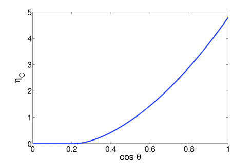
Figure 4: Graph of the function $\eta_{C}$ versus $\cos\theta$.

Since there is no a priori correlation between the direction of $\mathbf{B}$ and the orientation of the cubic lattice, it seems reasonable to associate to our model of plasma the critical parameter $\eta^{M}$ which is obtained by averaging the function $\eta_{C}(\cos\theta)$ over the full solid angle. One thus finds with a numerical integration

$$\eta^{M}=\int_{0}^{1}\eta_{C}(\cos\theta)d(\cos\theta)\cong 1.40\,.$$

Recalling the definition (2) of the parameter $\eta$, we conclude that to any given value of $B$ one can associate a critical value $n_{e}^{M}$ of the electronic density given by (1), with $\eta^{M}\cong 1.40$. For densities above this threshold, unstable normal modes are expected to arise within the plasma in a significant way.

By means of a more extensive study of the behavior of the matrix $\widehat{\mathbf{M}}(\mathbf{q})$ as a function of $\mathbf{q}$, it is possible to show that there exist also unstable modes for which the wave propagates along other lattice directions. However, the case considered in this section, for which $\mathbf{q}$ is parallel to a lattice axis, is the most significant one, since for any such $\mathbf{q}$ there are two independent transversally polarized unstable modes. Moreover, the instability of these modes can be removed by the presence of a suitable external magnetic field. This is precisely the mechanism which is responsible for the prediction of a density limit proportional to the squared magnetic field.

Of course, we could have taken a different Bravais lattice, instead of a simple cubic one, as the equilibrium configuration of the electrons. In such a case, the number and the properties of the unstable modes would in general have been different, since the matrix $\widehat{\mathbf{M}}(\mathbf{q})$ depends on the specific geometry of the lattice. As a consequence, also the value of the critical parameter $\eta^{M}$ is expected to be dependent on the choice of the equilibrium lattice. However, a systematic investigation of this dependence falls outside the scope of the present work.

IV The electrodynamical extension of the model

IV.1 The equation for the normal modes

The characteristic feature of the present approach consists in linearizing the equations of motion of the classical plasma model about an equilibrium configuration. By considering purely coulombian interactions, we have exhibited the existence of instabilities at short wavelengths which were not revealed by other treatments of the model. In the present section we want to show that, on the other hand, the present approach exactly reproduces for long wavelengths the dispersion relations which are usually obtained for cold plasmas by applying the continuum equations of MHD or the methods of references bg1 ; bp1 ; pb2 .

To this end, we note that the analytical treatment of plasma oscillations in the dipole approximation, which has been given in section II for purely coulombian interactions, can be generalized in a straightforward way so as to make use of the full electrodynamical expression of the field, thus taking into account also radiative terms and retardation. This amounts to replacing the electrostatical expression (7) of the dipole field with the complete one (see for instance chapter 9 of ref. Jackson )

$$\mathbf{E}_{\mathbf{m}}(\mathbf{x},t)= -\frac{e}{4\pi\epsilon_{0}}\bigg{[}3\frac{({\mathbf{x}}_{\mathbf{m}}\cdot{\mathbf{y}}){\mathbf{y}}}{y^{5}}-\frac{{\mathbf{x}}_{\mathbf{m}}}{y^{3}}+3\frac{(\dot{\mathbf{x}}_{\mathbf{m}}\cdot{\mathbf{y}}){\mathbf{y}}}{cy^{4}}$$

$$-\frac{\dot{\mathbf{x}}_{\mathbf{m}}}{cy^{2}}+\frac{(\ddot{\mathbf{x}}_{\mathbf{m}}\cdot{\mathbf{y}}){\mathbf{y}}}{c^{2}y^{3}}-\frac{\ddot{\mathbf{x}}_{\mathbf{m}}}{c^{2}y}\bigg{]}\,,$$ (28)

where $\mathbf{y}=\mathbf{x}-{\mathbf{r}}_{\mathbf{m}}$. In this formula the vector ${\mathbf{x}}_{\mathbf{m}}$ and all its time derivatives are evaluated at the retarded time $t_{\rm ret}=t-y/c$. The resulting equations for a normal mode essentially coincide with those obtained in reference mcg , so we will here limit ourselves to briefly recalling the results. By summing the retarded fields $\mathbf{E}_{\mathbf{m}}$ generated by all the individual electrons $\mathbf{m}\neq\mathbf{n}$, we obtain in place of (10)

$${\mathbf{e}}_{\mathbf{n}}^{(1)}({\mathbf{r}}_{\mathbf{n}},t)= \left[-\frac{en_{e}}{\epsilon_{0}}\widehat{\mathbf{M}}({\mathbf{q}},f)\cdot{\mathbf{C}}+\frac{ie\omega^{3}}{6\pi\epsilon_{0}c^{3}}{\mathbf{C}}\right]$$

$$\times\exp\left[i({\mathbf{k}}\cdot{\bf r}_{{\bf n}}-\omega t)\right]\,,$$ (29)

where $\widehat{\mathbf{M}}({\mathbf{q}},f)$ is a dimensionless symmetric matrix which depends on the rescaled wavevector $\mathbf{q}\equiv\mathbf{k}a/2\pi$ and the rescaled frequency $f\equiv\omega a/2\pi c$. A remarkable fact is that $\widehat{\mathbf{M}}({\mathbf{q}},f)$ is real when its arguments $\mathbf{q}$ and $f$ are real. Moreover, the term $(ie\omega^{3}/6\pi\epsilon_{0}c^{3}){\mathbf{C}}$ inside the square brackets of (IV.1) is exactly cancelled by the term $(e^{2}/6\pi\epsilon_{0}c^{3})\,\dddot{\mathbf{z}}_{\mathbf{n}}$ which, according to the Lorentz–Dirac equation (see dirac ; marino and chapter 17 of Jackson ), has to be added to the right-hand side of the equation of motion (3) in order to take into account radiation reaction. Comments on the profound mathematical and physical meaning of this cancellation are given in references cg and mcg . It has however to be noted that, in any case, the strength of the radiation reaction is completely negligible as far as the study of the dispersion relations in a plasma is concerned.

It is useful to decompose the matrix $\widehat{\mathbf{M}}$ as

$$\widehat{\mathbf{M}}({\mathbf{q}},f)=\widehat{\mathbf{M}}^{\rm lw}({\mathbf{q}},f)+\widehat{\mathbf{N}}({\mathbf{q}},f)\,,$$

where $\widehat{\mathbf{M}}^{\rm lw}({\mathbf{q}},f)$ is the dominant term for long-wavelengths, i.e. for $q\ll 1$, while $\widehat{\mathbf{N}}({\mathbf{q}},f)$ is a short-wavelength term, which becomes relevant only when $a$ is not negligible with respect to the wavelength $\lambda=2\pi/k$. For an isotropic lattice one obtains

$$\widehat{\mathbf{M}}^{\rm lw}({\mathbf{q}},f)=\widehat{\mathbf{M}}^{\rm mac}({\mathbf{k}},\omega)+\frac{\widehat{\mathbf{1}}}{3}\,,$$ (30)

where $\widehat{\mathbf{1}}$ is the $3\times 3$ identity matrix, and

$$M_{ij}^{\rm mac}({\mathbf{k}},\omega)=\frac{\omega^{2}\delta_{ij}-c^{2}k_{i}k_{j}}{c^{2}{\mathbf{k}}^{2}-\omega^{2}}=\frac{f^{2}\delta_{ij}-q_{i}q_{j}}{{\mathbf{q}}^{2}-f^{2}}$$

is the term associated with the macroscopic field ${\mathbf{E}}^{\rm mac}$ inside the plasma. In the long-wavelength limit we have in fact

$${\mathbf{E}}^{\rm mac}(\mathbf{x},t)=-\frac{en_{e}}{\epsilon_{0}}\widehat{\mathbf{M}}^{\rm mac}({\mathbf{k}},\omega)\cdot\mathbf{C}\exp\left[i({\mathbf{k}}\cdot\mathbf{x}-\omega t)\right]\,.$$

We have finally for the short-wavelength part:

$$N_{ij}({\mathbf{q}},f)=\ [(\alpha/3-2\beta){\bf q}^{2}-(2\alpha/3)f^{2}]\delta_{ij}$$

$$+(\alpha-4\beta)q_{i}q_{j}+2(5\beta-\alpha)q_{i}^{2}\delta_{ij}$$

$$-\sum_{\mathbf{m}\neq 0}\bar{c}_{ij}(\mathbf{H}_{\mathbf{m}},\mathbf{q},f)\,,$$ (31)

where the function $\bar{c}_{ij}$ is obtained by subtracting to the function

$$c_{ij}(\mathbf{H},\mathbf{q},f)=\frac{(H_{i}+q_{i})(H_{j}+q_{j})-f^{2}\delta_{ij}}{({\bf H}+{\bf q})^{2}-f^{2}}$$

the terms of order $k\leq 3$ of its Taylor expansion in the variables $\mathbf{q}/H$ and $f/H$ about the origin. This implies that in the long wavelength limit (i.e. $q\ll 1$, $f\ll 1$) $\bar{c}_{ij}$ is of order four in the variables $q$ and $f$. It follows that in this limit the leading term of $\widehat{\mathbf{N}}({\mathbf{q}},f)$ is represented by the second-degree homogeneous polynomial appearing on the right-hand side of (IV.1).

From these results, one deduces that the linearized dynamical equation for a normal mode is

$$i\frac{\omega e}{m_{e}}\mathbf{B}\times\mathbf{C}-\omega^{2}\mathbf{C}$$

$$=\ \omega_{p}^{2}[\widehat{\mathbf{M}}^{\rm mac}({\mathbf{k}},\omega)+\widehat{\mathbf{N}}({\mathbf{q}},f)]\cdot\mathbf{C}\,,$$ (32)

which represents the generalization of (16) when the full electrodynamic interaction is taken into account.

IV.2 The Coulomb limit

It is now interesting to establish under which conditions the purely coulombian equation (16) represents a good approximation of (IV.1). We first note in this respect that the proportionality factor $\beta$ between $f$ and $\tilde{\omega}=\omega/\omega_{c}$ is $\beta=f/\tilde{\omega}=\omega_{c}a/2\pi c=(\omega_{c}r_{e}/2\pi^{2}\eta c)^{1/3}$, where $\eta=\omega_{p}^{2}/\omega_{c}^{2}$, while $r_{e}=e^{2}/4\pi\epsilon_{0}m_{e}c^{2}$ is the so-called classical electron radius. In all experimental situations, one always has $\omega_{c}\ll c/r_{e}\cong 1.06\times 10^{23}$ Hz (i.e. $B\ll 10^{11}$ T), whence $\beta\ll 1$. For instance, for $\eta=3$ and $\omega_{c}\approx 10^{12}$ Hz, which is a typical value for a tokamak, we find $\beta\approx 5\times 10^{-5}$. It follows that, for all dispersion curves discussed in section III, for which $\tilde{\omega}$ was at most of order unity, one has $f=\beta\tilde{\omega}\ll 1$. This implies that, for wavelengths not too much longer than the lattice parameter, $f$ is negligible with respect to $q$. Hence, with very good approximation one can operate the substitution $\widehat{\mathbf{M}}({\mathbf{q}},f)\to\widehat{\mathbf{M}}({\mathbf{q}},0)$, and it is immediate to see that $\widehat{\mathbf{M}}({\mathbf{q}},0)$ is just the matrix $\widehat{\mathbf{M}}({\mathbf{q}})$ we introduced in section II. In particular, for $f\to 0$ we have $M_{ij}^{\rm mac}({\mathbf{k}},\omega)\to-q_{i}q_{j}/{\mathbf{q}}^{2}$ and $\widehat{\mathbf{N}}({\mathbf{q}},f)\to\widehat{\mathbf{N}}({\mathbf{q}},0)=\widehat{\mathbf{N}}({\mathbf{q}})$, where $\widehat{\mathbf{N}}({\mathbf{q}})$ is the matrix defined by (II.2). It follows that the dynamical equation (IV.1) reduces to (16) in this approximation. We have thus verified that the formulas derived by considering purely coulombian interactions give a fully satisfactory description of the dispersion relations discussed in section III.

IV.3 The long-wavelength limit

Let us now examine the form of the dispersion relations in the long-wavelength limit $\lambda\gg a$. In this case $q\ll 1$, so that $f$ in general is no longer negligible with respect to $q$. On the other hand, as we have already observed, in this limit $\widehat{\mathbf{N}}({\mathbf{q}},f)$ can be neglected, so that (IV.1) can be simplified as

$$i\frac{\omega e}{m_{e}}\mathbf{B}\times\mathbf{C}-\omega^{2}\mathbf{C}=\omega_{p}^{2}\widehat{\mathbf{M}}^{\rm mac}({\mathbf{k}},\omega)\cdot\mathbf{C}\,.$$ (33)

It is then easy to see that (33) leads to the same dispersion relations as those which are provided by the usual macroscopic treatment of high frequency waves in a magnetized plasma.

For instance, let us consider modes with $\mathbf{k}$ parallel to $\mathbf{B}$. If $\mathbf{C}$ is parallel to $\mathbf{k}$, then $\mathbf{B}\times\mathbf{C}=0$ and $\widehat{\mathbf{M}}^{\rm mac}({\mathbf{k}},\omega)\cdot\mathbf{C}=-\mathbf{C}$. It then follows from (33) that longitudinal waves (i.e. waves which involve an oscillation of the electronic density) have frequency $\omega=\omega_{p}$ independently of the magnetic field $B$ and of the wavelength $\lambda$, for $\lambda\gg a$. Hence $\omega_{p}$ plays indeed the role of “plasma frequency” also in this model. Moreover, for transversal waves, i.e. $\mathbf{C}\cdot\mathbf{k}=0$, we find that the normal modes allowed by (33) correspond to circularly polarized waves with dispersion relation

$$\frac{c^{2}k^{2}}{\omega^{2}}=1-\frac{\omega_{p}^{2}}{\omega(\omega-\omega_{c})}\,.$$ (34)

This result exactly coincides with that obtained in the approximation of MHD at zero temperature, represented by formula (17.35) and figures 17.4–17.5 of reference gold .

Similarly, let us consider the modes with $\mathbf{k}$ perpendicular to $\mathbf{B}$ and $k\ll 1/a$. For $\mathbf{C}$ parallel to $\mathbf{B}$, we deduce from (33) the existence of transversal waves unaffected by the magnetic field, with dispersion relation

$$c^{2}k^{2}=\omega^{2}-\omega_{p}^{2}\,.$$ (35)

These modes correspond to formula (16.32) and figure 16.4 of gold . In addition, for $\mathbf{C}\cdot\mathbf{B}=0$ we have modes in which the electrons describe elliptical orbits in planes orthogonal to $\mathbf{B}$. For these modes, (33) provides the dispersion relation

$$\frac{c^{2}k^{2}}{\omega^{2}}=1-\frac{\omega_{p}^{2}(\omega^{2}-\omega_{p}^{2})}{\omega^{2}(\omega^{2}-\omega_{p}^{2}-\omega_{c}^{2})}\,,$$ (36)

which corresponds to formula (17.12) and figure 17.1 of gold .

The behavior of the dispersion curves in the long-wavelength limit, for $\mathbf{B}$ either parallel or perpendicular to $\mathbf{k}$, is shown in the left part of Fig. 3 for $\omega_{p}^{2}/\omega_{c}^{2}=3$. In order to compare the scales of the abscissa in the two graphs of this figure, recall that, for $\omega_{c}\approx 10^{12}$ Hz, we have $\omega_{c}a/2\pi c\approx 5\times 10^{-5}$, so that $kc/\omega_{c}=10$ corresponds to $q=ka/2\pi\approx 5\times 10^{-4}$. This means that the long-wavelength region, represented in the left graph of Fig. 3, appears so narrow in the right graph that it becomes practically invisible. It is clear however that the left graph displays the behavior for low $k$ of the curves of the right graph. It has to be noted in particular that equation (33) is satisfied for $\mathbf{C}\cdot\mathbf{k}=0$ and $\omega=0$ independently of $k$, provided $k\ll 1/a$. Solutions of this type simply correspond to static deformations of the equilibrium lattice, and represent the limit for $q\ll 1$ of the lowest solid curve in the right part of Fig. 3.

V Conclusion

The main result obtained in this paper is that the classical model of a neutral plasma (as constituted by point electrons with Coulomb interactions, moving in a smeared-out positive background), when linearized about an equilibrium position, generally presents unstable normal modes. A relevant part of these modes is stabilized by an external magnetic field only for plasma densities below a maximal one, which is expressed by a Brillouin-type formula.

A natural question is then whether our result, which essentially refers to a zero temperature situation inasmuch as it deals with normal modes about an equilibrium configuration, may be significant also for high temperature plasmas. Indeed, it is well known that disruptive instabilities occur beyond a density limit in fusion machines with magnetic confinement green . In this connection one may remark that we are dealing here with an instability property, and that the raising of temperature tends to increase disorder rather than creating order. Thus the occurrence of an instability at zero temperature should imply instability at high temperatures as well.

An indication that the instability discussed here for the linearized system might perhaps be of interest for fusion plasmas, comes from the remark that the density limit found here turns out in several cases to be in a fairly good agreement with the limit empirically encountered in the operation of the tokamaks for fusion research. For example, for a magnetic field $B$ = 5 T the Alcator C-Mod device shows a limit $n_{e}^{M}\simeq 3.8\times 10^{20}$ m^-3 labombard , whereas formula (1), with $\eta^{M}\simeq 1.4$ as obtained for a simple cubic lattice, predicts $n_{e}^{M}\simeq 3.4\times 10^{20}$ m^-3. Analogously, at $B$ = 2 T, the DIII-D device petrie presents a density limit of $n_{e}^{M}\simeq 6\times 10^{19}$ m^-3, which has to be compared to the prediction $n_{e}^{M}\simeq 5.4\times 10^{19}$ m^-3 of formula (1).

Although a $B^{2}$ dependence of the density limit had been noticed by Granetz granetz for the Alcator C experiment, it is generally believed that the currently available global set of experimental data on the density limit of toroidal machines is best fitted by Greenwald’s empirical scaling law green , according to which the limit is proportional to the plasma current density in the tokamak. However, it must be recalled that, despite the large theoretical work on the subject, at the moment no widely accepted, first principles model for the density limit in tokamak devices appears to exist green . Thus, the results here presented might provide a motivation for further experimental investigations, in order to establish whether a quadratical dependence on the magnetic field may provide a good description of the data for at least some class of machines. This might have relevant implications on the expected performances of future tokamaks.

Appendix A Calculation of the field acting on an electron

We start from the expression of the charge density within the plasma

$$\rho(\mathbf{x},t)=e\sum_{\mathbf{n}}\delta^{3}(\mathbf{x}-\mathbf{z}_{\mathbf{n}}(t))+\rho_{\rm bg}\,.$$

Up to first order in $\mathbf{c}\equiv\mathbf{C}\exp(-i\omega t)$, we can write $\rho=\rho^{(0)}+\rho^{(1)}$, where

$$\rho^{(0)}(\mathbf{x}) =\frac{e}{V}-e\sum_{\mathbf{n}}\delta^{3}(\mathbf{x}-\mathbf{r}_{\mathbf{n}})$$

$$=-\frac{e}{V}\sum_{\mathbf{m}\neq\mathbf{0}}\exp(i\mathbf{G}_{\mathbf{m}}\cdot\mathbf{x})\,,$$

$$\rho^{(1)}(\mathbf{x},t) =e\sum_{\mathbf{n}}\exp(i\mathbf{k}\cdot\mathbf{r}_{\mathbf{n}})\,\mathbf{c}\cdot\mathbf{\nabla}\delta^{3}(\mathbf{x}-\mathbf{r}_{\mathbf{n}})$$

$$=i\frac{e}{V}\sum_{\mathbf{m}}\mathbf{c}\cdot(\mathbf{G}_{\mathbf{m}}+\mathbf{k})\exp[i(\mathbf{G}_{\mathbf{m}}+\mathbf{k})\cdot\mathbf{x}]\,.$$

In these formulas, the vectors

$$\mathbf{G}_{\mathbf{m}}\equiv\frac{2\pi}{V}(m_{1}\mathbf{a}_{2}\times\mathbf{a}_{3}+m_{2}\mathbf{a}_{3}\times\mathbf{a}_{1}+m_{3}\mathbf{a}_{1}\times\mathbf{a}_{2})\,,$$

with $\mathbf{m}\in\mathbf{Z}^{3}$, represent the points of the reciprocal lattice.

Using the Poisson equation $\Delta\phi=-\rho/\epsilon_{0}$, we obtain for the electrostatic potential $\phi$ the corresponding expansion $\phi=\phi^{(0)}+\phi^{(1)}$, where

$$\phi^{(0)}(\mathbf{x})=-\frac{e}{V\epsilon_{0}}\sum_{\mathbf{m}\neq\mathbf{0}}\frac{\exp(i\mathbf{G}_{\mathbf{m}}\cdot\mathbf{x})}{\mathbf{G}_{\mathbf{m}}^{2}}\,,$$ (37)

$$\phi^{(1)}(\mathbf{x},t)=\frac{ie}{V\epsilon_{0}}\sum_{\mathbf{m}}\left.\frac{\mathbf{c}\cdot\mathbf{G}^{\prime}_{\mathbf{m}}}{|\mathbf{G}^{\prime}_{\mathbf{m}}|^{2}}\,\exp(i\mathbf{G}^{\prime}_{\mathbf{m}}\cdot\mathbf{x})\right|_{\mathbf{G}^{\prime}_{\mathbf{m}}=\mathbf{G}_{\mathbf{m}}+\mathbf{k}}\,.$$

It follows that the electric field inside the plasma is given in the dipole approximation by $\mathbf{E}=\mathbf{E}^{(0)}+\mathbf{E}^{(1)}$, where

$$\mathbf{E}^{(0)}(\mathbf{x})=-\mathbf{\nabla}\phi^{(0)}(\mathbf{x})=\frac{ie}{V\epsilon_{0}}\sum_{\mathbf{m}\neq\mathbf{0}}\frac{\mathbf{G}_{\mathbf{m}}}{\mathbf{G}_{\mathbf{m}}^{2}}\exp(i\mathbf{G}_{\mathbf{m}}\cdot\mathbf{x})\,,$$

$$\mathbf{E}^{(1)}(\mathbf{x},t)=-\mathbf{\nabla}\phi^{(1)}(\mathbf{x},t)=\frac{e}{V\epsilon_{0}}\sum_{\mathbf{m}}\left.\frac{\mathbf{c}\cdot\mathbf{G}^{\prime}_{\mathbf{m}}}{|\mathbf{G}^{\prime}_{\mathbf{m}}|^{2}}\mathbf{G}^{\prime}_{\mathbf{m}}\,\exp(i\mathbf{G}^{\prime}_{\mathbf{m}}\cdot\mathbf{x})\right|_{\mathbf{G}^{\prime}_{\mathbf{m}}=\mathbf{G}_{\mathbf{m}}+\mathbf{k}}\,.$$ (38)

The contribution due to the electron $\mathbf{n}$ is $\mathbf{E}_{\mathbf{n}}=\mathbf{E}^{(0)}_{\mathbf{n}}+\mathbf{E}^{(1)}_{\mathbf{n}}$, where

$$\mathbf{E}^{(0)}_{\mathbf{n}}(\mathbf{x})=\frac{e}{4\pi\epsilon_{0}}\frac{\mathbf{x}-\mathbf{r}_{\mathbf{n}}}{|\mathbf{x}-\mathbf{r}_{\mathbf{n}}|^{3}}=\frac{ie}{(2\pi)^{3}\epsilon_{0}}\int d^{3}\mathbf{p}\frac{\mathbf{p}}{p^{2}}\exp[i\mathbf{p}\cdot(\mathbf{x}-\mathbf{r}_{\mathbf{n}})]\,,$$

$$\mathbf{E}^{(1)}_{\mathbf{n}}(\mathbf{x},t)=\frac{e}{4\pi\epsilon_{0}}\exp(i\mathbf{k}\cdot\mathbf{r}_{\mathbf{n}})\bigg{[}\frac{\mathbf{c}}{|{\mathbf{x}}-{\mathbf{r}}_{\mathbf{n}}|^{3}}-3\frac{{\mathbf{c}}\cdot({\mathbf{x}}-{\mathbf{r}}_{\mathbf{n}})}{|{\mathbf{x}}-{\mathbf{r}}_{\mathbf{n}}|^{5}}({\mathbf{x}}-{\mathbf{r}}_{\mathbf{n}})\bigg{]}=\frac{e}{(2\pi)^{3}\epsilon_{0}}\exp(i\mathbf{k}\cdot\mathbf{r}_{\mathbf{n}})\int d^{3}\mathbf{p}\frac{\mathbf{c}\cdot\mathbf{p}}{p^{2}}\mathbf{p}\,\exp[i\mathbf{p}\cdot(\mathbf{x}-\mathbf{r}_{\mathbf{n}})]\,.$$ (39)

Using (38) and (39), and proceeding as in mcg , we thus obtain

$${\mathbf{e}}_{\mathbf{n}}^{(1)}({\mathbf{r}}_{\mathbf{n}},t)= \lim_{{\bf x}\rightarrow{\bf r}_{{\bf n}}}\left[{\bf E}^{(1)}({\bf x},t)-{\bf E}_{\bf n}^{(1)}({\bf x},t)\right]=\frac{e}{V\epsilon_{0}}\exp(i\mathbf{k}\cdot\mathbf{r}_{\mathbf{n}})\lim_{{\bf x}\rightarrow{\bf 0}}\int d^{3}{\bf p}\,e^{i{\bf p\cdot x}}\frac{\mathbf{p}\cdot\mathbf{c}}{p^{2}}\mathbf{p}\left[\sum_{{\bf m}}\delta^{3}({\bf p-H}_{{\bf m}}-{\bf q})-1\right]$$

$$= -\frac{en_{e}}{\epsilon_{0}}\widehat{\mathbf{M}}({\mathbf{q}})\cdot\mathbf{c}\exp(i\mathbf{k}\cdot\mathbf{r}_{\mathbf{n}})\,,$$

where $\mathbf{q}=\mathbf{k}a/2\pi$, $\mathbf{H}_{\mathbf{m}}=\mathbf{G}_{\mathbf{m}}a/2\pi$, and

$$\widehat{\mathbf{M}}({\mathbf{q}})=-\lim_{\eta\rightarrow 0^{+}}\int d^{3}{\bf p}\,e^{-\eta p^{2}}c_{ij}(\mathbf{p},\mathbf{q})\left[\sum_{{\bf m}}\delta^{3}(\mathbf{p}-\mathbf{H}_{\bf m})-1\right]\,.$$

The above integral can be evaluated by expanding the integrand function $c_{ij}(\mathbf{p},\mathbf{q})$, defined by formula (15), in powers of $\mathbf{q}/p$ about the origin. Denoting by $c_{ij}^{(k)}$ the term of order $(q/p)^{k}$, the first four terms of this expansion are respectively

$$c_{ij}^{(0)} =\frac{p_{i}p_{j}}{p^{2}}\,,$$

$$c_{ij}^{(1)} =\frac{1}{p^{2}}\left(q_{i}p_{j}+q_{j}p_{i}-2{\bf q}\cdot{\bf p}\frac{p_{i}p_{j}}{p^{2}}\right)\,,$$

$$c_{ij}^{(2)} =\frac{1}{p^{2}}\bigg{\{}q_{i}q_{j}-2(q_{i}p_{j}+q_{j}p_{i})\frac{{\bf q}\cdot{\bf p}}{p^{2}}+\frac{p_{i}p_{j}}{p^{2}}\left[-{\bf q}^{2}+\frac{4({\bf q}\cdot{\bf p})^{2}}{p^{2}}\right]\bigg{\}}\,,$$

$$c_{ij}^{(3)} =\frac{1}{p^{4}}\bigg{\{}-2{\bf q}\cdot{\bf p}\,q_{i}q_{j}+(q_{i}p_{j}+q_{j}p_{i})\left[-{\bf q}^{2}+\frac{4({\bf q}\cdot{\bf p})^{2}}{p^{2}}\right]-4\frac{p_{i}p_{j}}{p^{2}}{\bf q}\cdot{\bf p}\left[-{\bf q}^{2}+\frac{2({\bf q}\cdot{\bf p})^{2}}{p^{2}}\right]\bigg{\}}\,.$$

The limit for $\eta\to 0^{+}$ of the integral of these four terms gives a polynomial function of $\mathbf{q}$ whose coefficients can be evaluated numerically for any given lattice geometry. The remainder $\bar{c}_{ij}\equiv c_{ij}-c_{ij}^{(0)}-c_{ij}^{(1)}-c_{ij}^{(2)}-c_{ij}^{(3)}$ of the integrand function is of order $(q/p)^{4}$ for $p\to+\infty$, hence it is possible to put directly $\eta=0$ before evaluating the integral. This procedure leads for an isotropic lattice to formulas (10) and (12)–(II.2), with

$$\alpha =\lim_{\eta\rightarrow 0^{+}}\left(-\sum_{{\bf m}\neq{\bf 0}}\frac{\exp\left(-\eta{\bf H}_{{\bf m}}^{2}\right)}{{\bf H}_{{\bf m}}^{2}}+\frac{2\pi^{3/2}}{\sqrt{\eta}}\right)\,,$$ (40)

$$\beta =\lim_{\eta\rightarrow 0^{+}}\left(-\sum_{{\bf m}\neq{\bf 0}}\frac{\left({\bf H}_{{\bf m}}\right)_{1}^{4}}{\left|{\bf H}_{{\bf m}}\right|^{6}}\exp\left(-\eta{\bf H}_{{\bf m}}^{2}\right)+\frac{2\pi^{3/2}}{5\sqrt{\eta}}\right)\,.$$ (41)

Note that for an isotropic lattice one can also write

$$\sum_{\mathbf{m}\neq 0}\bar{c}_{ij}(\mathbf{H}_{\mathbf{m}},\mathbf{q})=\lim_{L\to+\infty}\sum_{\mathbf{m}\neq 0,|\mathbf{m}|\leq L}\tilde{c}_{ij}(\mathbf{H}_{\mathbf{m}},\mathbf{q})\,,$$

where

$$\tilde{c}_{ij}(\mathbf{H},\mathbf{q})=\frac{(H_{i}+q_{i})(H_{j}+q_{j})}{({\bf H}+{\bf q})^{2}}-\frac{\delta_{ij}}{3}-\frac{q_{i}q_{j}+{\bf q}^{2}\delta_{ij}/3-2q_{i}^{2}\delta_{ij}}{{\mathbf{H}}^{2}}+\frac{2H_{1}^{4}}{H^{6}}(2q_{i}q_{j}+{\bf q}^{2}\delta_{ij}-5q_{i}^{2}\delta_{ij})\,.$$

Appendix B Calculation of the electrostatic energy at equilibrium

From formula (18) it follows that the electrostatic energy of our model of plasma in its equilibrium configuration is

$$U_{0}=-\frac{Ne}{2}\lim_{\mathbf{x}\to\mathbf{0}}\left[\phi^{(0)}(\mathbf{x})+\frac{e}{4\pi\epsilon_{0}x}\right]\,,$$

where $\phi^{(0)}$ is the potential generated by all the charges of the plasma, given by (37), while $-e/4\pi\epsilon_{0}x$ is the potential generated by the electron at the origin.

In order to numerically compute $U_{0}$, it is convenient to introduce the auxiliary electrostatic potential $\psi$ generated by an array of charge distributions, each given by the superposition of a point charge $-e$ and a gaussian of total charge $+e$. This can formally be written as

$$\psi(\mathbf{x})=\sum_{\mathbf{n}}\bar{\psi}(\mathbf{x}-\mathbf{r}_{\mathbf{n}})\,,$$

where $\mathbf{r}_{\mathbf{n}}$ are the points of the Bravais lattice, and the function $\bar{\psi}$ satisfies

$$\Delta\bar{\psi}(\mathbf{x})=\frac{e}{\epsilon_{0}}\left[\delta^{3}(\mathbf{x})-\left(\frac{\eta}{\pi}\right)^{3/2}\exp(-\eta x^{2})\right]\,,$$ (42)

$\eta$ being an arbitrary parameter. We have $U_{0}=A+B$, where

$$A=-\frac{Ne}{2}\lim_{\mathbf{x}\to\mathbf{0}}\left[\psi(\mathbf{x})+\frac{e}{4\pi\epsilon_{0}x}\right]$$

and

$$B=-\frac{Ne}{2}\lim_{\mathbf{x}\to\mathbf{0}}\left[\phi^{(0)}(\mathbf{x})-\psi(\mathbf{x})\right]\,.$$

We are now going to show that both terms $A$ and $B$ can be evaluated as the sums of rapidly convergent series.

A standard integration of (42) provides

$$\bar{\psi}(\mathbf{x})=-\frac{eF(\sqrt{\eta}x)}{4\pi\epsilon_{0}x}\,,$$

where the function $F$ is defined by (21). We have

$$\lim_{\mathbf{x}\to\mathbf{0}}\left[\bar{\psi}(\mathbf{x})+\frac{e}{4\pi\epsilon_{0}x}\right] =\frac{e}{4\pi\epsilon_{0}}\lim_{x\to 0}\frac{1-F(\sqrt{\eta}x)}{x}$$

$$=\frac{e\sqrt{\eta}}{2\epsilon_{0}\pi^{3/2}}\,,$$

whence

$$A=-\frac{Ne^{2}}{8\pi\epsilon_{0}}\left[2\sqrt{\frac{\eta}{\pi}}-\sum_{\mathbf{n}\neq\mathbf{0}}\frac{F(\sqrt{\eta}|\mathbf{r}_{\mathbf{n}}|)}{|\mathbf{r}_{\mathbf{n}}|}\right]\,.$$ (43)

In order to calculate $B$, we observe that, due to its lattice periodicity, $\psi$ can be Fourier expanded as

$$\psi(\mathbf{x})=\sum_{\mathbf{m}}\tilde{\psi}_{\mathbf{m}}\exp(i\mathbf{G}_{\mathbf{m}}\cdot\mathbf{x})\,,$$ (44)

where $\mathbf{G}_{\mathbf{m}}$ are the points of the reciprocal lattice, and

$$\tilde{\psi}_{\mathbf{m}}=\frac{1}{V}\int\bar{\psi}(\mathbf{x})\exp(-i\mathbf{G}_{\mathbf{m}}\cdot\mathbf{x})d^{3}\mathbf{x}\,.$$

We have

$$\tilde{\psi}_{\mathbf{0}}= -\frac{e}{\epsilon_{0}V}\int_{0}^{+\infty}F(\sqrt{\eta}x)x\,dx$$

$$= -\frac{e}{\epsilon_{0}V}\sqrt{\frac{\eta}{\pi}}\int_{0}^{+\infty}e^{-\eta x^{2}}x^{2}\,dx=-\frac{e}{4\epsilon_{0}V\eta}$$

and, for $\mathbf{m}\neq\mathbf{0}$,

$$\tilde{\psi}_{\mathbf{m}}= -\frac{e}{\epsilon_{0}V|\mathbf{G}_{\mathbf{m}}|}\int_{0}^{+\infty}F(\sqrt{\eta}x)\sin(|\mathbf{G}_{\mathbf{m}}|x)dx$$

$$= -\frac{e}{\epsilon_{0}V|\mathbf{G}_{\mathbf{m}}|^{2}}\left[1-\sqrt{\frac{\eta}{\pi}}\int_{-\infty}^{+\infty}e^{-\eta x^{2}}\cos(|\mathbf{G}_{\mathbf{m}}|x)dx\right]$$

$$= -\frac{e}{\epsilon_{0}V|\mathbf{G}_{\mathbf{m}}|^{2}}\left[1-\exp\left(-\frac{|\mathbf{G}_{\mathbf{m}}|^{2}}{4\eta}\right)\right]\,.$$

From (37) and (44) it then follows that

$$B =\frac{Ne}{2}\left[\tilde{\psi}_{\mathbf{0}}+\sum_{\mathbf{m}\neq\mathbf{0}}\left(\tilde{\psi}_{\mathbf{m}}-\frac{e}{\epsilon_{0}V|\mathbf{G}_{\mathbf{m}}|^{2}}\right)\right]$$

$$=-\frac{Ne^{2}}{2\epsilon_{0}V}\left[\frac{1}{4\eta}-\sum_{\mathbf{m}\neq\mathbf{0}}\frac{1}{|\mathbf{G}_{\mathbf{m}}|^{2}}\exp\left(-\frac{|\mathbf{G}_{\mathbf{m}}|^{2}}{4\eta}\right)\right]\,.$$ (45)

By putting $\xi=a^{2}\eta/\pi$, from (43) and (B) one finally obtains (19), with $b$ given by (II.3).

Appendix C Calculation of $\eta_{C}(\theta)$

The equation ${\rm det}\,\widehat{\mathbf{A}}(\mathbf{k},\omega)=0$, with $\widehat{\mathbf{A}}(\mathbf{k},\omega)$ given by (17) and $\mathbf{q}=(1/2)\mathbf{u}_{3}$ , can be explicitly written as

$$u^{3}-(1+\eta)u^{2}-\eta[\eta Z(3Z+2)+Z-\xi]u$$

$$-\eta^{3}Z^{2}(1+2Z)=0\,,$$ (46)

with $u=\widetilde{\omega}^{2}=\omega^{2}/\omega_{c}^{2}$, $Z\equiv\bar{N}(1/2)\cong 0.05212$, and $\xi\equiv(1+3Z)\cos^{2}\theta$. We see that the left-hand side of this equation is a third-degree polynomial in $u$, which we shall call $P(u)$. Hence the corresponding normal modes will all be stable (i.e. have a real frequency) provided this polynomial admits three real nonnegative roots. We first note that $P(0)<0$ for all $\eta>0$. A necessary condition for the existence of three positive roots is then $P^{\prime}(0)>0$, where $P^{\prime}$ denotes the derivative of $P$. Hence we must have

$$\eta<\frac{\xi-Z}{Z(3Z+2)}\,,$$ (47)

which implies in particular $\xi>Z$, i.e. $\cos\theta>\sqrt{Z/(1+3Z)}\cong 0.2123$. Whenever (47) is satisfied, it is easily seen that $P^{\prime}(u)$ has two positive roots, which we shall call $u_{1}$ and $u_{2}$, with $0<u_{1}<u_{2}$. Then $P(u)$ will have three positive roots if and only if $P(u_{1})>0$ and $P(u_{2})<0$. With some simple algebra, one sees that the validity of both these conditions is equivalent to the single inequality

$$4\xi Z(1+3Z)^{3}\eta^{3}-[Z^{2}(1+3Z)^{2}-2Z\xi(18Z^{2}+21Z+5)$$

$$+(36Z^{2}+24Z+1)\xi^{2}]\eta^{2}-2[Z^{2}(1+Z)-Z(4+9Z)\xi$$

$$+(1+6Z)\xi^{2}-2\xi^{3}]\eta-Z^{2}+2Z\xi-\xi^{2}<0\,.$$ (48)

It is found that, for $\xi>Z$, the third degree polynomial in $\eta$ on the left-hand side of (C) has a single positive root $\bar{\eta}$, and that this root satisfies (47). Putting $\eta_{C}(\theta)=\bar{\eta}$, it then follows that (C) admits three real nonnegative roots for all $\eta$ such that $0\leq\eta\leq\eta_{C}(\theta)$.

References

• (1) L. Brillouin, Phys. Rev. 67, 260 (1945).
• (2) R. C. Davidson, Physics of Nonneutral Plasmas (Addison-Wesley, Redwood City, 1990).
• (3) D. Bohm and E. P. Gross, Phys. Rev. 75, 1851 and 1864 (1949).
• (4) D. Bohm and D. Pines, Phys. Rev. 82, 625 (1951).
• (5) D. Pines and D. Bohm, Phys. Rev. 85, 338 (1952).
• (6) I. Langmuir, Proc. Nat. Acad. Sci. 14, 627 (1928).
• (7) L. Tonks and I. Langmuir, Phys. Rev. 33, 195 (1929).
• (8) J. D. Jackson, Classical Electrodynamics (John Wiley & Sons, New York, 1975).
• (9) M. Marino, A. Carati and L. Galgani, Ann. Phys. 322, 799 (2007).
• (10) C. Kittel, Introduction to Solid State Physics, eighth edition (John Wiley & Sons, Hoboken, 2005).
• (11) P.A.M. Dirac, Proc. R. Soc. London 167, 148 (1938).
• (12) M. Marino, Ann. Phys. 301, 85 (2002).
• (13) A. Carati and L. Galgani, Nuovo Cimento 118 B, 839 (2003).
• (14) R. J. Goldston and P.H. Rutherford, Introduction to Plasma Physics (IOP Publishing, Bristol, 1995).
• (15) M. Greenwald, Plasma Phys. Control. Fusion 44, R27 (2002).
• (16) B. LaBombard et al., Phys. Plasmas 8, 2107 (2001).
• (17) T. W. Petrie, A. G. Kellmann and M. Ali Mahdavi, Nucl. Fusion 33, 929 (1993).
• (18) R. S. Granetz, Phys. Rev. Lett. 49, 658 (1982).