Quantum compacton vacuum

Abstract

We study the properties of classical and quantum compacton chains by means of extensive numerical simulations. Such chains are strongly nonlinear and their classical dynamics remains chaotic at arbitrarily low energies. We show that the collective excitations of classical chains are described by sound waves which decay rate scales algebraically with the wave number with a generic exponent value. The properties of the quantum chains are studied by the quantum Monte Carlo method and it is found that the low energy excitations are well described by effective phonon modes with the sound velocity dependent on an effective Planck constant. Our results show that at low energies the quantum effects lead to a suppression of chaos and drive the system to a quasi-integrable regime of effective phonon modes.

I I. Introduction

The investigation of nonlinear chains, started by Fermi, Pasta and Ulam in 1955 fpu , still remains an active and interesting area of research which attracts a significant interest of nonlinear community (see e.g. reviews flach ; lepri ; gallavotti ; ruffo and Refs. therein). Usually, in such chains the nonlinear terms are relatively weak compared to the linear ones and strong nonlinear effects appear only at sufficiently high energy excitations.

However, there are also other types of chains where the linear modes are absent and the dynamics is strongly nonlinear at arbitrarily small energies. In such chains a time can be rescaled with energy and hence the system always remains in a strongly nonlinear regime. A prominent example is the Hertz lattice which describes elastically interacting hard balls where the elasticity parameter scales as a square-root of the displacement nesterenko1983 ; fauve ; chatterjee ; porter corresponding to the nonlinearity index $n=5/2$. Nesterenko nesterenko1983 ; nesterenko1985 ; nesterenko1994 ; nesterenko2001 described a compact traveling-wave solution in the Hertz lattice now known as compacton. A rigorous mathematical description of compactons was given by Rosenau and Hyman rosenau1 ; rosenau2 for a class of nonlinear partial differential equations (PDEs) with nonlinear dispersion. A detailed analysis of compacton dynamics on lattices with various nonlinearity index has been performed recently in ahnert . It was shown that on a finite lattice interactions between compactons lead to chaotic dynamics characterized by a spectrum of positive Lyapunov exponents. A well known example of such compacton chain is the toy “Newton’s cradle” ahnert .

In the compacton lattice the dynamics is chaotic at arbitrarily small energies when more than one compacton are exited. Therefore it is interesting to understand what happens in such quantum lattices and what are the properties of quantum compacton vacuum. The studies of such quantum chains are reported in this work. We use the quantum Monte Carlo (QMC) method and the approach developed for the quantum Frenkel-Kontorova model as it is described in qfk . The aim of this work is to understand the properties of quantum compacton vacuum and low energy excitations. It is interesting to note that the recent progress with cold atoms allowed to realize a quantum Newton’s cradle dweiss and to study energy redistribution between atoms. The experimental progress stimulated also theoretical studies of integrability and non-integrability in one-dimensional atomic lattices at high energy excitations olshanii . In contrast to that we study the properties of vacuum and low energy excitations in quantum compacton lattices when the linear terms are absent and nonlinearity is always strong in the classical case. Thus the classical dynamics of such compacton chain is always chaotic ahnert (except a special case of one compacton moving in a lattice). What are the properties of the quantum compacton chain is the subject of studies of this work.

The paper is organized as follows: the model description is given in Section II, the properties of sound waves in the classical compacton chains are analyzed in Section III, simple analytical estimates for the compacton chain are presented in Section IV, numerical results of the QMC are presented in Section V and the results are summarized in Section VI.

II II. Model description

The quantum compacton chain is described by the Hamiltonian

$$\hat{H}=\sum_{l=1}^{M}\frac{1}{2}\hat{p}_{l}^{2}+\frac{\alpha}{n}(\hat{x}_{l}-\hat{x}_{l-1})^{n}$$ (1)

where index $l$ marks $M$ particles in the chain and $n$ is the nonlinearity index. Here $x_{l}$ gives the particle coordinate counted from the equilibrium distance between particles which is taken to be $a$. For the Newton cradle $a$ is given by the ball diameter. We use the dimensionless units in which the particle mass is equal to unity and the momentum $p_{l}$ gives the particle velocity. For the quantum problem the operators of momentum and coordinate have the usual commutator $[\hat{p}_{l},\hat{x}_{l^{\prime}}]=-i\hbar\delta_{l,l^{\prime}}$ with a dimensionless Planck constant $\hbar$. We assume the periodic boundary conditions with $x_{l}=x_{l+M}$, $p_{l}=p_{l+M}$ or fixed ends boundary conditions. The later is a specific case of even number of particles $M=2N$. We note that the particles are distinguishable since they are located at well defined positions.

Let us remind few known results for the harmonic chain at $n=2$. By a canonical transformation to normal modes $\hat{P}_{k}=\frac{1}{\sqrt{N}}\sum_{l}\hat{p}_{l}\mathrm{e}^{-2\pi\mathrm{i}lk/M}$, $\hat{Q}_{k}=\frac{1}{\sqrt{N}}\sum_{l}\hat{x}_{l}\mathrm{e}^{2\pi\mathrm{i}lk/M}$ the Hamiltonian (1) takes the form

$$\hat{H} = \frac{1}{2}\sum_{k}\left(\left|\hat{P}_{k}\right|^{2}+{\omega_{k}}^{2}\left|\hat{Q}_{k}\right|^{2}\right)$$ (2)

with the normal mode frequencies $\omega_{k}=2\bar{\omega}\sin(q_{k}/2)$, $\bar{\omega}=\sqrt{\alpha}$ and wave numbers $q_{k}=\pi k/N$, $k=1,\ldots,N-1$. Here and below we use the fixed boundary conditions with $x_{l=0}=x_{l=N}=0$ and $N$ particles.

It is convenient to introduce sine modes via relations $\hat{S}_{k}=\sqrt[]{\frac{2}{N}}\sum_{l}\sin(q_{k}l)\hat{x}_{l}$, $\hat{x}_{l}=\sqrt[]{\frac{2}{N}}\sum_{k}\sin(q_{k}l)\hat{S}_{k}$. The vacuum state of the chain is a product of vacuum states of all modes. For any mode in the vacuum state one has an average of mode energy $\hat{U}_{k}$ being $\left\langle\hat{U}_{k}\right\rangle=\omega^{2}_{k}\left\langle\hat{S}^{2}_{k}\right\rangle/2=\hbar\omega_{k}/4$ and hence

$$\left\langle\hat{S}_{k}\hat{S}_{k^{\prime}}\right\rangle=\frac{\hbar}{2\omega_{k}}\delta_{kk^{\prime}}.$$ (3)

Thus different harmonics are independent and as a result the squared deviation from equilibrium for a particle $l$ is $\left\langle\hat{x}_{l}^{2}\right\rangle=\frac{2}{N}\sum_{k=1}^{N-1}\sin^{2}(q_{k}l)\left\langle\hat{S}^{2}_{k}\right\rangle=\frac{\hbar}{N}\sum_{k=1}^{N-1}\sin^{2}(q_{k}l)/\omega_{k}$. For the central particle $l=N/2$ the displacement diverges logarithmically with the chain length $\left\langle\hat{x}_{l}^{2}\right\rangle=\frac{\hbar}{4n}\sum_{k=1}^{N-1}1/\sin(q_{k}/2)\approx\frac{\hbar}{\pi}\ln(2/q_{\min})$, where $q_{\min}\equiv q_{k=1}=\pi/N$. For $\hbar=1$ the displacement is of the order of unity for $N\sim 30$. We will assume that such displacements are small compared to the distance $a$ between particles.

The spacial correlator of the chain can be also explicitly calculated as $\left\langle\hat{x}_{l}\hat{x}_{l+\Delta}\right\rangle=\frac{2}{N}\sum_{k=1}^{N-1}\sin(q_{k}l)\sin(q_{k}(l+\Delta))\left\langle\hat{S}_{k}^{2}\right\rangle$ where the brackets note the quantum average. Using (3) we obtain after summation over all $l$

$$\left\langle\hat{x}_{l}\hat{x}_{l+\Delta}\right\rangle_{l}\approx\frac{\hbar}{N}\sum_{k=1}^{N-1}\frac{\cos(q_{k}\Delta)}{4\sin(q_{k}/2)}$$ (4)

At finite temperature $T$ the relation (3) is modified for the usual expression for bosons

$$\left\langle\hat{S}_{k}^{2}\right\rangle=\frac{\hbar}{\omega_{k}}\left(\frac{1}{2}+\frac{1}{\exp(\hbar\omega_{k}/T)-1}\right).$$ (5)

With this form of $\left\langle\hat{S}_{k}^{2}\right\rangle$ one can obtain the expression for the correlator $\left\langle\hat{x}_{l}\hat{x}_{l+\Delta}\right\rangle$ at finite temperature.

The properties of the chain can be also characterized by the static form factor defined as

$$F(q)=\left\langle\left|\sum_{l}\exp\left(\mathrm{i}(a\cdot l+\hat{x}_{l})q/\hbar\right)\right|^{2}\right\rangle\;,$$ (6)

where $q$ can be viewed as a momentum transfer during a process of photon scattering, and $a$ is the spacing of the chain lattice.

Before to start the studies of the quantum compacton problem at $n>2$ we consider in the next Section the propagation of sound waves in the classical chain at $n=4$.

III III. Sound waves in classical compacton lattices

To find the spectrum of sound waves and their decay rates we simulate numerically the dynamics of classical system (1) at $n=4$, $\alpha=1$ with the periodic boundary conditions. The simulations are done with a Runge-Kutta-Nystrom method with time step $0.02$. Initially a random distribution of momenta $p_{l}$ is seeded, so that the total energy per particle is 1. After a transient of time $T_{trans}=10$ a perturbation of the type $x_{l}\to x_{l}+\varepsilon\cos q_{k}l$ is imposed with $\varepsilon=0.1$. The wave number $q_{k}$ is changed in the range $0<q_{k}<\pi$. The corresponding Fourier mode of $x_{l}$ changes in time approximately as $f_{q}\propto e^{-\gamma_{q}t}\cos\omega_{q}t$. This time dependence is obtained from an ensemble of particles. We use up to $10^{7}$ particles in an ensemble to obtain good averaging of statistical fluctuations.

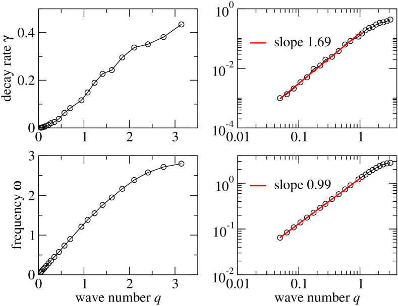
Figure 1: (Color online) Bottom panels: spectrum of waves $\omega(q)$ in the classical compacton lattice (1) at $n=4$, $\alpha=1$ and energy per particle $\langle E_{l}\rangle$ equal to unity, at small wave numbers $q$ the spectrum is close to a linear law of sound waves $\omega\propto q$. Top panels: decay rate of sound waves $\gamma(q)$, at small $q$ we have $\gamma\propto q^{\beta}$ with $\beta\approx 1.69$. Left panels are in normal scale, right panels are in log-log scale, fits are shown by straight lines with indicated slopes.

The numerical results are shown in Fig. 1 for the spectrum of sound waves $\omega(q)$ and their decay rates $\gamma(q)$. The frequency spectrum is close to the spectrum of sound in a harmonic lattice $\omega(q)=2\bar{\omega}\sin q/2$ with $\bar{\omega}\approx 1.4$. At small $q$ we have the spectrum of sound waves. The effective velocity of sound for phonon like excitations is given by $\bar{\omega}\approx 1.4\langle\alpha E_{l}\rangle^{1/4}$. Here the dependence on a given average energy per particle $\langle E_{l}\rangle$ appears since a typical frequency of particle oscillations is proportional to $\langle E_{l}\rangle^{1/4}$. The speed of sound in the physical lattice with distance $a$ between particles is $c=\bar{\omega}a$. The decay rate of these waves drops algebraically with the decrease of the wave vector $q$ as $\gamma\propto q^{\beta}$. We obtain the value $\beta\approx 1.69$ that is close to the generic exponent $\beta=5/3$ for the decay rate in nonlinear lattices (see e.g. lepri ). Thus even if the dynamics inside a compacton lattice is strongly chaotic (see ahnert ) the long wave oscillation properties of the whole lattice are well described by effective sound waves. In a certain sense the situation is similar to sound in a gas media: each particle moves chaotically but the collective long wave excitations are well described by sound waves.

It is interesting to note that recently a localization of sound waves in a random three-dimensional elastic network of metallic balls has been observed experimentally in skipetrov . Such a system can be viewed as a random three-dimensional Newton’s cradle. However, our studies here are restricted to the one-dimensional case.

IV IV. Simple estimates for quantum compacton chains

The sound velocity $c$ in a gas is given by the derivative of pressure $p$ over the gas mass density $\rho$ at fixed entropy $S$ (adiabatic process): $c^{2}=\left(\frac{\partial p}{\partial\rho}\right)_{S}$. Since the pressure is proportional to the force $p\propto\partial U/\partial x_{l}$, hence, $c^{2}\propto\partial^{2}U/\partial^{2}x_{l}$. This leads to a simple estimate for the sound velocity based on the virial theorem according to which $2\left\langle K\right\rangle=n\left\langle U\right\rangle$, where $K$ and $U$ are particle kinetic and potential energies and brackets mark their average values. Since the temperature is proportional to the kinetic energy we have $T\sim\left\langle K\right\rangle=n\left\langle U\right\rangle=\alpha\left\langle(x_{i}-x_{j})^{n}\right\rangle\sim\alpha(\Delta x)^{n}$ where $\Delta x$ is an average displacement of a particle. This gives

$$c^{2}=\omega^{2}a^{2}\sim a^{2}U^{{}^{\prime\prime}}(\Delta x)\sim a^{2}\alpha^{2/n}T^{1-2/n}\;.$$ (7)

For the classical case this expression agrees with the above analytical results for $\bar{\omega}$ for $n=2,4$.

For the quantum compacton chain we can use the Heisenberg uncertainty relation $p\sim\hbar/\Delta x$ for the minimization of the ground state energy $E=\hbar^{2}/2(\Delta x)^{2}+\alpha(\Delta x)^{n}/n$ that gives $\Delta x\sim(\hbar^{2}/\alpha)^{1/(n+2)}$, and $\omega^{2}\sim\alpha(\Delta x)^{n-2}=\alpha^{4/(n-2)}\hbar^{2(n-2)/(n+2)}$. As a result the sound velocity of the quantum chain is

$$c^{2}\sim a^{2}\alpha^{4/(n-2)}\hbar^{2(n-2)/(n+2)}$$ (8)

For $n=2$ this velocity is independent of $\hbar$ but for $n>2$ it decreases with $\hbar$ that corresponds to the decrease of the ground state energy of a nonlinear oscillator. The properties of the ground state are analyzed in the numerical simulations presented in the next Section.

V V. Numerical results of quantum Monte Carlo

V.1 A. Method description

For our numerical simulations of quantum chain (1) we use the Metropolis algorithm (MA) metropolis in the Euclidean time $\tau$ related to the system temperature $T=\hbar/\tau$. The simulations are done in the same way as for the studies of the quantum Frenkel-Kontorova model described in qfk . A general description of this QMC method can be found in girvin .

The paths in the discretized Euclidean time are generated by the statistical sum

$$\sum_{\{x_{l,j}\}}\exp\left\{-\sum_{l,j}\left[\frac{1}{2\Delta\tau}(x_{l,j}-x_{l,j-1})^{2}+\frac{\Delta\tau}{2n}(x_{l,j}-x_{l-1,j})^{n}\right]\right\}$$ (9)

which links the problem to a statistical mechanics for configuration distribution of some lattice of $N\times N_{\tau}$ size where $N$ is number of particles and $N_{\tau}=\tau/\Delta\tau$ is number of discrete steps of size $\Delta\tau$ in the Euclidean time interval $\tau$. As usual the periodic boundary conditions are used in this time with $x_{l}(\tau_{j}+\tau)=x_{l}(\tau_{j})$ and $\tau_{j}=j\Delta\tau$. In our numerical studies we use up to $N_{\tau}=1000$, $\tau=200$ and up to $2\cdot 10^{6}$ Metropolis updates. We fix $\alpha=1$ for numerical simulations.

The numerical simulations assume a generation of configurations $\{x_{k,j}\}$ with probability proportional to their weights in the statistical sum. The Metropolis method looks very efficient, providing an update step gives rather large modifications for a give site. However, corresponding modifications are local and are dominated by the nearest neighbor sites, that results in a significant slowdown for long wave configurations. Thus it is useful to combine the Metropolis method with the microcanonic dynamics (MCD) method. The MCD method is a noiseless algorithm and it works as follows: all variables $x_{l,m}$ are considered as some coordinates, and the sum

$$\sum_{l,j}\left[\frac{1}{2\Delta\tau}(x_{l,j}-x_{l,j-1})^{2}+\frac{\Delta\tau}{2n}(x_{l,j}-x_{l-1,j})^{n}\right]\equiv\mathcal{U}(x)$$ (10)

as a potential energy of a certain system. Then, a set of auxiliary momentum variables $\{{\cal P}_{l,j}\}$ is added and the equations of motion are solved numerically in an auxiliary update “time” variable $u$:

$$\partial{{\cal P}}_{l,j}/\partial{u} = -\frac{\partial\mathcal{U}}{\partial x_{l,j}}=\nabla_{l,j}\mathcal{U}(x)$$

$$\partial{x}_{l,j}/\partial{u} = {\cal P}_{l,j}\;.$$ (11)

With this dynamical description the system evolves over some iso-energy hypersurface in the phase space, and we get an ensemble of configurations.

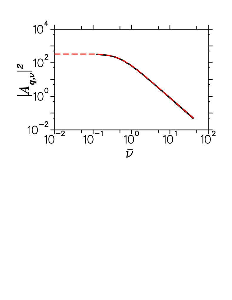
Figure 2: (Color online) Typical data for the Fourier harmonics $|A_{q_{j},\nu_{m}}|^{2}$ and its fit by the dependence (14); black curve shows numerical data, dashed red/gray curve shows the fit (curves are overlapped). Data correspond to the linear chain at $n=2$, $\hbar=1$,  $q_{j}=10\pi/N$, $N=64$, $\tau_{\max}=100$, $N_{\tau}=1000$.

However, an obvious disadvantage of such a method is that one needs to solve the differential equations numerically with a step which becomes smaller for decreasing $\Delta\tau$, due to the terms $\mathcal{U}(x)$ with $\Delta\tau$ in the denominator. But even worse, these terms act as some noise that reduces the relaxation rate along $l$ (space dimension). Thus, in order to accelerate the relaxation processes we introduce into $\mathcal{U}(x)$ a parameter $C_{K}$

$$\mathcal{U}(x;C_{K})=\sum_{l,j}\left[\frac{C_{K}}{2\Delta\tau}(x_{l,j}-x_{l,j-1})^{2}+\frac{\Delta\tau}{2n}(x_{l,j}-x_{l-1,j})^{n}\right].$$ (12)

Then the update step is organized as follows:
a) the fast mixing stage, with $C_{K}=\Delta\tau$, at which the smallness of denominator is canceled, here the MCD method is applied during the auxiliary “time” interval $u\sim 100$;
b) return to $C_{K}=1$ and application of the Metropolis updates at maximum 400 updates.

Such a combined approach allows us to reduce significantly the number of Metropolis updates and to have more rapid numerical simulations. We checked that both methods (only MA steps and MA steps combined with the MCD method) give the same results.

V.2 B. Quantum excitations above the compacton vacuum

The ensemble of quantum paths, obtained by the numerical methods described above, determines the properties of the vacuum ground state of the system. Averages of various quantities over this ensemble give the corresponding average observables at this state. However, the study of fluctuations of quantum paths allows us to extract a more interesting information about the spectrum of low energy elementary excitations.

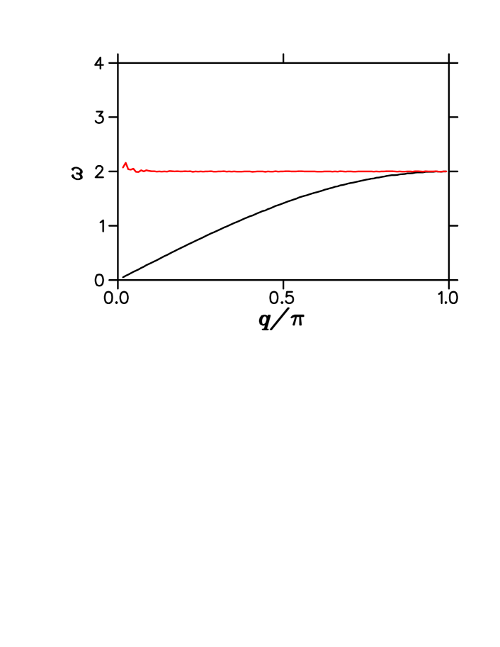
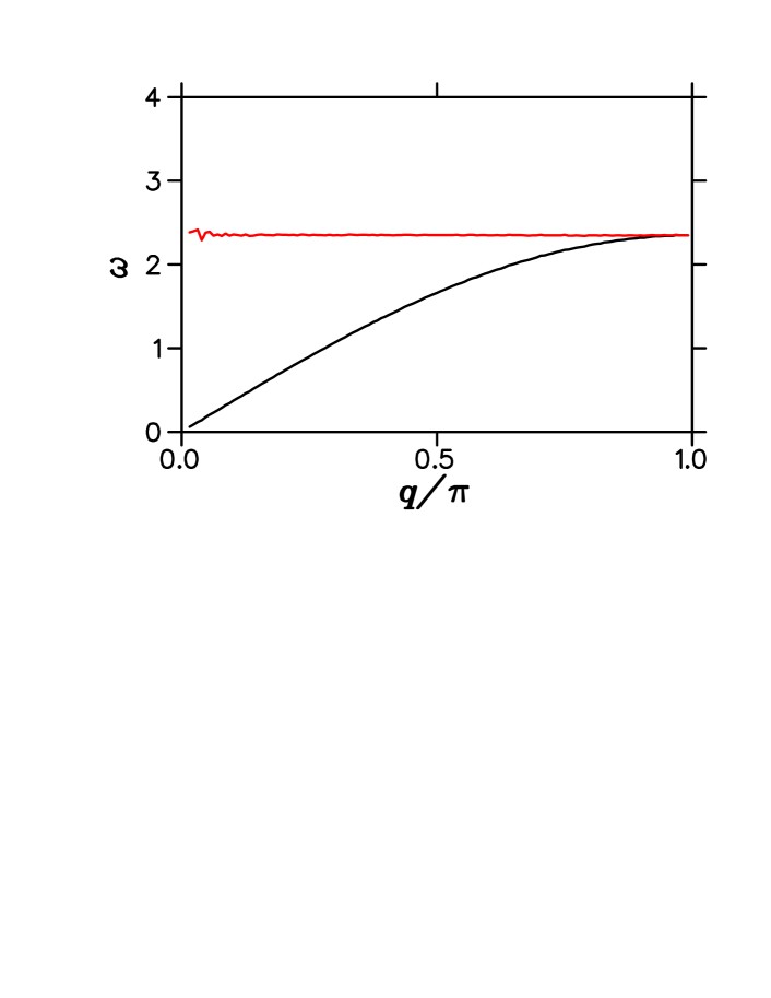
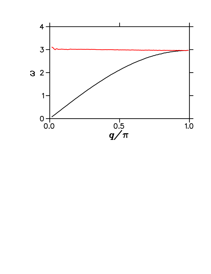
Figure 3: (Color online) Spectra of quantum phonon modes shown by black bottom curve and obtained from QMC simulations for $n=2$ (top panel), $n=4$ (middle panel) and $n=8$ (bottom panel); top red/gray curve shows the ratio $\omega/\sin(q/2)$ for each panel. The data are obtained at $\hbar=1$, $N=128$, $N_{\tau}=1000$, $\tau_{\max}=200$, the simulations are done with MA using $2\cdot 10^{6}$ updates.

To extract this information we consider the Fourier harmonics of quantum paths

$$A_{q_{j},\nu_{m}}=\sum_{l,k}x_{l,k}\sin(q_{j}l)\exp({\mathrm{i}}\mathrm{\nu_{m}}\tau_{k})$$ (13)

where $q_{j}=\pi j/N$, $j=1,\ldots,N-1$, $\tau_{k}=k\Delta\tau$, $\nu_{m}=2\pi m/\tau_{\max}$, $m=0,\ldots,N_{\tau}/2$. One expects a Lorentzian distribution in frequency $\omega$ for exponential decay of quasiparticle excitations in the imaginary time:

$$\left\langle|A_{q_{j},\nu_{m}}|^{2}\right\rangle=\frac{\hbar}{2}\frac{1}{\omega^{2}+\bar{\nu}_{m}^{2}}.$$ (14)

Here we use the renormalized frequency $\bar{\nu}_{m}=\frac{2}{\Delta\tau}\sin(\nu_{m}\Delta\tau/2)$ with the sine term appearing due to the discreetness of time steps. The fit of data for $A_{q_{j},\nu_{m}}$ allows to find the spectral dependence $\omega=\omega(q_{j})$ and thus to determine the dispersion law of elementary quantum excitations. A typical example of such a fit is shown in Fig. 2.

The spectrum of low energy excitations extracted via such a procedure is shown in Fig. 3 for $n=2,4,8$. For $n=2$ the data reproduce the theoretical result for a harmonic chain with $\bar{\omega}=\omega(q)/(2\sin(q/2))=1$. For $n=4,8$ this form of spectrum is preserved with a moderate renormalization of $\bar{\omega}\approx 1.2,1.5$ respectively. This shows that even if the classical compacton chain is fully chaotic the quantum compacton vacuum is rather regular and is characterized by the phonon type excitations rather similar to the case of a harmonic chain.

Figure 4: The dependence of sound velocity $c$  on $\hbar$. Squares, triangles and circles correspond to $n=2$, $4$ and $8$, respectively. The straight lines show the fit dependence (see text). Parameters of simulations are: $N=64$, $\tau_{\max}=100$, $N_{\tau}=1000$. Logarithms are natural.

Our data show that $\bar{\omega}$ varies with $\hbar$ and $n$. This leads to the dependence of the sound velocity $c=d\omega/dq$ on these two parameters. The numerically obtained dependence of $c$ on $\hbar$ is shown in Fig. 4. The fit by an algebraic dependence $c\propto\hbar^{\eta}$ gives $\eta=0.33;0.56$ for $n=4,8$ respectively. These numerical values are close to the theoretical power from Eq. (8) with $\eta=(n-2)/(n+2)$ corresponding to $\eta=1/3,3/5$ for these $n$ values. The global variation of the whole spectrum $\omega(q)$ with $\hbar$ is shown in Fig. 5 for $n=4$.

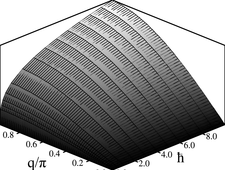
Figure 5: Spectra of quantum phonon modes for the quartic chain at $n=4$. Data correspond to $N=64$, $\tau=100$, $N_{\tau}=1000$, and to the interval $\hbar=0.063-10$,  extrapolated smoothly from $\hbar=0.063$ to $\hbar=0$.

Trying to find deviations from a harmonic chain behavior we compute numerically the amplitudes of phonon modes $S_{q}^{2}$ (see Eq. (3) with $q=k/(N-1)$) and the correlation function $\left\langle x_{l}x_{l+\Delta}\right\rangle_{l}$ (see Eq. (4)). The results are shown in Fig. 6. For $n=2$ the numerical data are in a good agreement with the theory for a harmonic chain. For $n=4,8$ our numerical data show the dependencies rather similar to the case of a harmonic chain with slight vertical shift which can be attributed to the modified values of $\bar{\omega}$ discussed above. We note that for the case of $T>0$ the theoretical formulas (3), (4) are computed with the expression (5) for bosons at finite temperature. Since the value of $\tau$ in Fig. 6 is rather large there is no significant difference between the theoretical expressions for $T=0$ and $T=\hbar/\tau$.

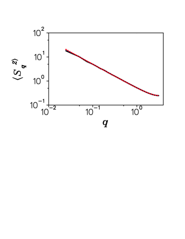
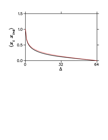
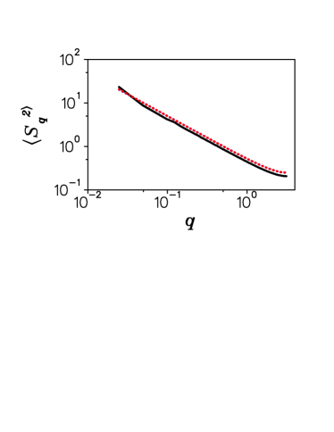
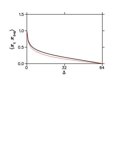
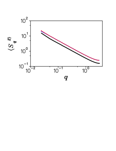
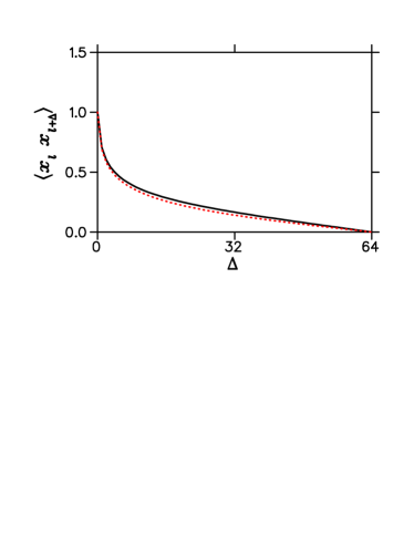
Figure 6: (Color online) Left column: Amplitudes of phonon modes, see Eq.(3), for $n=2$ (top), $4$ (middle), $8$ (bottom). Right column: Normalized correlation function, see Eq.(4), for $l=64$ (central particle) for the same order of panels. Other parameters $\hbar=1$, $N=128$, $N_{\tau}=1000$, $\tau=200$. Simulations include $2\cdot 10^{6}$ updates. Red/gray and blue/black dotted curves give the theoretical expectations for harmonic chain with temperature $T=\hbar/\tau$ and $T=0$, respectively (curves overlap).

An additional attempt to see deviations from a harmonic chain behavior is performed by computing the form factor $F(q)$ of the chain given by Eq. (6). However, the results presented in the left panel of Fig. 7 show that all three chains with $n=2,4,8$ give very similar curves for $F(q)$ which practically overlap.

The confirmation of similarity between these three types of chains in the ground state is given by the direct computation of the correlator $\left.K(q_{1},q_{2})\equiv\left\langle S_{q}S_{q^{\prime}}\right\rangle/(\left\langle S_{q}S_{q}\right\rangle\left\langle S_{q^{\prime}}S_{q^{\prime}}\right\rangle\right)^{1/2}$ which should be proportional to $\delta_{q_{1},q_{2}}$ according to (3). Indeed, the numerical data show a strong peak at $q_{1}=q_{2}$ with a residual noisy level of $K$ at other $q_{1}\neq q_{2}$ without any structural dependence on $q_{1},q_{2}$. This residual level can be characterized by the total weighted admixture of other modes to a given mode $q$ via

$$w(q)=\sum_{q^{\prime}\neq q}|\left\langle S_{q}S_{q^{\prime}}\right\rangle|^{2}/|\left\langle S_{q}S_{q}\right\rangle|^{2}\;.$$ (15)

This characteristic is shown in the right panel of Fig. 7 for $n=2,4,8$. The admixture $w(q)$ increases with $n$ but still it remains rather small for strongly nonlinear lattices with $n=4,8$. This gives one more confirmation that the quantum compacton vacuum is rather close to a harmonic one.

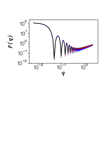
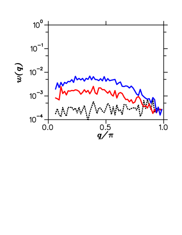
Figure 7: (Color online) Left panel: formfactor $F(q)$, see Eq.(6), for $n=2$ (black curve), $4$ (red/gray points), $8$ (blue/black points) (data practically coincide). Other parameters are as in Fig. 6 including $a=1$. Right panel: admixture to normal modes from other harmonics. Red/gray and blue/black curves show data for quartic and octic chains, the dotted black curve corresponds to linear chain and gives an estimate for a noise level. Data correspond to $\hbar=1$, $N=64$, $\tau=50$, $N_{\tau}=500$, number of independent quantum paths is $10^{4}$.

At finite temperatures the spectrum of excitations $\omega(q)$ and the amplitudes of phonon modes $S^{2}_{s}$ are still well approximated by the theoretical dependence for a harmonic chain as it is shown in Fig. 8 at $T=0.1$ which is about two times larger than the excitation energy for a mode with minimal frequency $\hbar\omega_{min}=\hbar\pi/N\approx 0.049$. The situation is found to be qualitatively the same when the temperature is increased up to $T=1$ keeping fixed other parameters of Fig. 8 even if at $n=8$ the splitting between the theoretical curve and the numerical data becomes more visible (due to a similarity of these data with Fig. 8 we do not show them here).

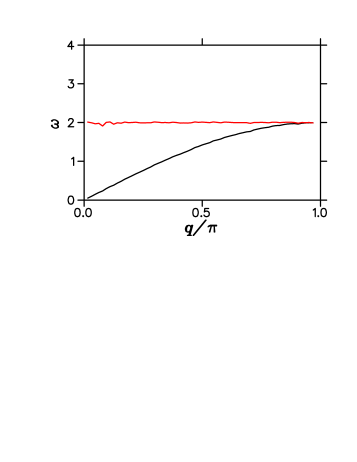
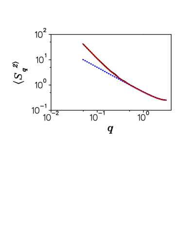
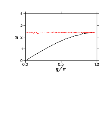
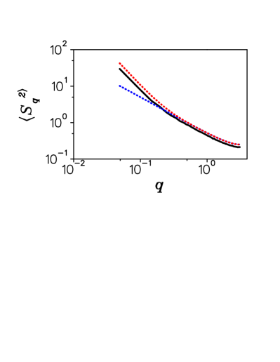
Figure 8: (Color online) Left column: spectra of quantum phonon modes at $T=0.1$ for $n=2$ (top) and $4$ (bottom) with the curves as in Fig. 3. Right column: Amplitudes of phonon modes, see Eq.(3) in the same order; red/gray and blue/black dotted lines give theoretical expectations for harmonic chain with temperature $T=\hbar/\tau$ and $T=0$, respectively. Other parameters are $\hbar=1$, $N_{\tau}=200$, $\tau_{\max}=10$. Simulations are done with combined MA and MCD method with $10^{4}$ Metropolis updates.

VI VI. Summary

In this work we investigated the properties of collective modes in nonlinear compacton chains. For the classical compacton chains we find that the chain has sound modes which decay rather slowly due to nonlinear wave interactions with the rate $\gamma\propto q^{\beta}$ with $\beta\approx 5/3$. This decay rate is in agreement with the generic result of decay of sound waves in one-dimensional nonlinear chains lepri .

On local scales the classical dynamics in such compacton chains is strongly chaotic. One could expect that this chaos may lead to nontrivial properties of quantized chains. However, our extensive numerical studies of quantum compacton vacuum show that it is characterized by low energy phonon excitations which are rather similar to those of a harmonic chain. The main difference is that the sound velocity of these phonon modes depends on an effective Planck constant as it is described by Eq. (8).

In a certain sense quantum effects suppress the signatures of classical chaos in the ground state. Such a phenomenon is known for quantum systems with a few degrees of freedom. For example, a ground state of a Sinai billiard can be rather well approximated by a Hartree-Fock trial function with one maximum so that the signatures of quantum chaos appear only in the semiclassical regime for highly excited states haake . This is more or less natural for systems with few degrees of freedom. Our case has infinite number of degrees of freedom but in spite of that the quantum compacton vacuum remains rather similar to a vacuum of a harmonic chain in which the oscillator frequency is dependent of an effective Planck constant. It is possible that certain signatures of such quasi-integrability at low energies find their manifestations in a slow chaotization of excitations in a quantum Newton’s cradle observed in experiments dweiss . However, we should note that such a statement can be considered only on a qualitative level of rigor since the model (1) at $n=4$ or $8$ gives only an approximate description of ball interactions (see discussion at ahnert ).

However, let us note that our methods are well adapted for analysis of low energy oscillatory quantum waves. It is possible that other approaches should be used to detect quantum chock wave type excitations with large displacements between two parts of the chain (in principle the energy of such type compacton like excitations is not very high and is independent of the lattice size). Other methods should be used to analyze such type of excitations.

It is possible that a degeneracy of chaos in a vicinity of quantum compacton vacuum is linked to the space homogeneity of the model (1). Indeed, the ground state of the quantum Frenkel-Kontorova model has much more rich properties qfk appearing due to a presence of periodic potential.

One of us (OVZ) is supported by the RAS joint scientific program “Fundamental problems in nonlinear dynamics” and thanks UMR 5152 du CNRS, Toulouse for hospitality during this work, another (DLS) thanks Univ. Potsdam for hospitality at the final stage of this work.

References

- (1) E. Fermi, J. Pasta, S. Ulam, and M. Tsingou, Los Alamos, Preprint LA-1940 (1955); E. Fermi, Collected Papers, Univ. of Chicago Press, Chicago, 2, 978 (1965).
- (2) S. Flach and C.R. Willis, Phys. Rep. 295, 181 (1998).
- (3) S. Lepri, R. Livi, and A. Politi, Phys. Rep. 377, 1 (2003).
- (4) G. Gallavotti (Ed.), The Fermi-Pasta-Ulam problem: a status report, Springer, Berlin (2007).
- (5) T. Dauxois and S. Ruffo, Fermi-Pasta-Ulam nonlinear lattice oscillations, Scholarpedia 3(8):5538 (2008).
- (6) V.F. Nesterenko, J. Appl. Mech. Tech. 24, 733 (1983).
- (7) C. Coste, E. Falcon, and S. Fauve, Phys. Rev. E 56, 6104 (1997).
- (8) A. Chatterjee, Phys. Rev. E 59, 5912 (1999).
- (9) M.A. Porter, C. Daraio, E.B. Herbold, I. Szelengowicz, and P. G. Kevrekidis, Phys. Rev. E 77, 015601(R) (2008).
- (10) A. N. Lazaridi and V. F. Nesterenko, J. Appl. Mech. Tech. Phys. 26, 405 (1985).
- (11) S. L. Gavrilyuk and V. F.Nesterenko, J. Appl. Mech. Tech. Phys. 34, 784 (1994).
- (12) V. Nesterenko, Dynamics of Homogeneous Materials, (Springer, New York, 2001).
- (13) P. Rosenau and J.M. Hyman, Phys. Rev. Lett. 70, 564 (1993).
- (14) P. Rosenau, Phys. Rev. Lett. 73, 1737 (1994).
- (15) K. Ahnert and A. Pikovsky, Phys. Rev. E 79, 026209 (2009).
- (16) O. V. Zhirov, G. Casati, and D. L. Shepelyansky, Phys. Rev. E 67, 056209 (2003).
- (17) T. Kinoshita, T. Wenger, and D. S. Weiss, Nature 440, 900 (2006).
- (18) V. A. Yurovsky, M. Olshanii, and D. S. Weiss, Adv. At. Mol. Opt. Phys. 55, 61 (2008).
- (19) H. Hu, A. Srtybulevych, J.H. Page, S.E. Skipetrov and B.A. van Tiggelen, Nature Physics 4, 945 (2008).
- (20) N. Metropolis, A. Rosenbluth, M. Rosenbluth, A. Teller, and E. Teller, J. Chem. Phys. 21, 1087 (1953).
- (21) S.L. Sondhi, S.M. Girvin, J.P. Caini, and D. Shahar, Rev. Mod. Phys. 69, 315 (1997).
- (22) F. Haake, Quantum signatures of chaos, Springer, Berlin (2001).