Hybrid Numerical Solution of the
Chemical Master Equation

Abstract

We present a numerical approximation technique for the analysis of continuous-time Markov chains that describe networks of biochemical reactions and play an important role in the stochastic modeling of biological systems. Our approach is based on the construction of a stochastic hybrid model in which certain discrete random variables of the original Markov chain are approximated by continuous deterministic variables. We compute the solution of the stochastic hybrid model using a numerical algorithm that discretizes time and in each step performs a mutual update of the transient probability distribution of the discrete stochastic variables and the values of the continuous deterministic variables. We implemented the algorithm and we demonstrate its usefulness and efficiency on several case studies from systems biology.

1 Introduction

A common dynamical model in systems biology is a system of ordinary differential equations (ODEs) that describes the time evolution of the concentrations of certain proteins in a biological compartment. This macroscopic model is based on the theory of chemical kinetics and assumes that the concentrations of chemical species in a well-stirred system change deterministically and continuously in time. It provides an appropriate description of a chemically reacting system as long as the numbers of molecules of the chemical species are large. However, in living cells the chemical populations can be low (e.g. a single DNA molecule, tens or a few hundreds of RNA or protein molecules). In this case the underlying assumptions of the ODE approach are violated and a more detailed model is necessary, which takes into account the inherently discrete and stochastic nature of chemical reactions [24, 30, 8, 27, 34]. The theory of stochastic chemical kinetics provides an appropriate description by means of a discrete-state Markov process, that is, a continuous-time Markov chain (CTMC) that represents the chemical populations as random variables [9, 10]. If $n$ is the number of different types of molecules, then we describe the state of the system at a certain time instant by an $n$-dimensional random vector whose $i$-th entry represents the number of molecules of type $i$. In the thermodynamic limit (when the number of molecules and the volume of the system approach infinity) the Markov model and the macroscopic ODE description are equal [21]. Therefore, the ODE approach can be used to approximate the CTMC only if all populations are large.

The evolution of the CTMC is given by a system of linear ordinary differential equations, known as the chemical master equation (CME). A single equation in the CME describes the time derivative of the probability of a certain state at all times $t\geq 0$. Thus, the solution of the CME is the probability distribution over all states of the CTMC at a particular time $t$, that is, the transient state probabilities at time $t$. The solution of the CME can then be used to derive measures of interest such as the distribution of switching delays [23], the distribution of the time of DNA replication initiation at different origins [26], or the distribution of gene expression products [35]. Moreover, many parameter estimation methods require the computation of the posterior distribution because means and variances do not provide enough information to calibrate parameters [15].

The more detailed description of chemical reactions using a CTMC comes at a price of significantly increased computational complexity because the underlying state space is usually very large or even infinite. Therefore, Monte Carlo simulation is in widespread use, because it allows to generate random trajectories of the model while requiring only little memory. Estimates of the measures of interest can be derived once the number of trajectories is large enough to achieve the desired statistical accuracy. However, the main drawback of simulative solution techniques is that a large number of trajectories is necessary to obtain reliable results. For instance, in order to halve the confidence interval of an estimate, four times more trajectories have to be generated. Consequently, often stochastic simulation is only feasible with a very low level of confidence in the accuracy of the results.

Recently, efficient numerical algorithms have been developed to compute an approximation of the CME [16, 25, 3, 5, 6, 13, 32, 7, 18]. Many of them are based on the idea of restricting the analysis of the model during a certain time interval to a subset of states that have “significant” probability. While some of these methods rely on an a priori estimation of the geometric bounds of the significant subset [16, 25, 3], others are based on a conversion to discrete time and they decide dynamically which states to consider at a certain time step [5, 6, 32].

If the system under consideration contains large populations, then the numerical algorithms mentioned above perform poorly. The reason is that the random variables that represent large populations have a large variance. Thus, a large number of states have a significant probability, which renders the numerical approximation of the distribution computationally expensive or infeasible.

In this paper we use a stochastic hybrid approach to efficiently approximate the solution of systems containing both small and large populations. More precisely, we maintain the discrete stochastic representation for small populations, but at the same time we exploit the small relative variance of large populations and represent them by continuous deterministic variables. Since population sizes change over time we decide dynamically ("on-the-fly") whether we represent a population by a continuous deterministic variable or keep the discrete stochastic representation. Our criterion for changing from a discrete to a continuous treatment of a variable and vice versa is based on a population threshold.

For the solution of the stochastic hybrid model, we propose a numerical approximation method that discretizes time and performs a mutual update of the distributions of the discrete stochastic variables and the values of the continuous deterministic variables. Hence, we compute the solution of a CME with a reduced dimension as well as the solution of a system of (non-linear) ordinary differential equations. The former describes the distribution of the discrete stochastic variables and the latter the values of the continuous deterministic variables, and the two descriptions depend on each other. Assume, for instance, that a system has two chemical species. The two population sizes at time $t$ are represented by the random variables $X(t)$ and $Y(t)$, where $X(t)$ is large and $Y(t)$ is small. Then, we consider for $Y(t)$ all events $Y(t)=y$ that have significant probability, i.e., $\mathit{Pr}\!\left(Y(t)=y\right)$ is greater than a certain threshold. For $X(t)$ we consider the conditional expectations $E[X(t)\,|\,Y(t)=y]$ and assume that they change continuously and deterministically in time. We iterate over small time steps $h>0$ and, given the distribution for $Y(t)$ and the values $E[X(t)\,|\,Y(t)=y]$, we compute the distribution of $Y(t+h)$ and the values $E[X(t+h)\,|\,Y(t+h)=y]$. Again, we restrict our computation to those values of $y$ that have significant probability.

To demonstrate the effectiveness of our approach, we have implemented the algorithm and applied it successfully to several examples from systems biology. Our most complex example has 6 different chemical species and 10 reactions. We compare our results with our earlier purely discrete stochastic approach and with the purely continuous deterministic approach in terms of running times and accuracy.

Related Work. Different hybrid approaches have been proposed in the literature [12, 31, 29]. As opposed to our approach, they focus on Monte Carlo simulation and consider the problem of multiple time scales. They do not use deterministic variables but try to reduce the computational complexity of generating a trajectory of the model by approximating the number of reactions during a certain time step. The closest work to ours is the hybrid approach proposed by Hellander and Lötstedt [14]. They approximate large populations by normally distributed random variables with a small variance and use Monte Carlo simulation to statistically estimate the probability distribution of the remaining populations with small sizes. They consider a single ODE to approximate the expected sizes of the large populations. As opposed to that, here we consider a set of ODEs to approximate the expected sizes of the large populations conditioned on the small populations. This allows us to track the dependencies between the different populations more acurately. Moreover, instead of a statistical estimation of probabilities, we provide a direct numerical method to solve the stochastic hybrid model. The direct numerical method that we use for the computation of the probability distributions of the stochastic variables has shown to be superior to Monte Carlo simulation [5]. Another difference is that the method in [14] does not allow a dynamic switching between stochastic and deterministic treatment of variables.

Finally, our approach is related to the stochastic hybrid models considered in [4, 2] and to fluid stochastic Petri nets [17]. These approaches differ from our approach in that they use probability distributions for the different values a continuous variable can take. In our setting, at a fixed point in time we only consider the conditional expectations of the continuous variables, which is based on the assumption that the respective populations are large and their relative variance is small. This allows us to provide an efficient numerical approximation algorithm that can be applied to systems with large state spaces. The stochastic hybrid models in [4, 2, 17] cannot be solved numerically except in the case of small state spaces.

2 Discrete-state Stochastic
Model

According to Gillespie’s theory of stochastic chemical kinetics, a well-stirred mixture of $n$ molecular species in a volume with fixed size and fixed temperature can be represented as a continuous-time Markov chain $\left(\mathbf{X}(t),t\geq 0\right)$ [9]. The random vector $\mathbf{X}(t)=\left(X_{1}(t),\ldots,X_{n}(t)\right)$ describes the chemical populations at time $t$, i.e., $X_{i}(t)$ is the number of molecules of type $i\in\{1,\ldots,n\}$. Thus, the state space of $\mathbf{X}$ is $\mathbb{Z}^{n}_{+}=\{0,1,\ldots\}^{n}$. The state changes of $\mathbf{X}$ are triggered by the occurrences of chemical reactions, which come in $m$ different types. For $j\in\{1,\ldots,m\}$ let $\mathbf{u}_{j}\in\mathbb{Z}^{n}$ be the change vector of the $j$-th reaction type, that is, $\mathbf{u}_{j}=\mathbf{u}_{j}^{-}+\mathbf{u}_{j}^{+}$ where $\mathbf{u}_{j}^{-}$ contains only non-positive entries that specify how many molecules of each species are consumed (reactants) if an instance of the reaction occurs and vector $\mathbf{u}_{j}^{+}$ contains only non-negative entries that specify how many molecules of each species are produced (products). Thus, if $\mathbf{X}(t)=\mathbf{x}$ for some $\mathbf{x}\in\mathbb{Z}^{n}_{+}$ with $\mathbf{x}+\mathbf{u}_{j}^{-}$ being non-negative, then $\mathbf{X}(t+dt)=\mathbf{x}+\mathbf{u}_{j}$ is the state of the system after the occurrence of the $j$-th reaction within the infinitesimal time interval $[t,t+dt)$.

As rigorously derived by Gillespie [10], each reaction type has an associated propensity function, denoted by $\alpha_{1},\ldots,\alpha_{m}$, which is such that $\alpha_{j}(\mathbf{x})\cdot dt$ is the probability that, given $\mathbf{X}(t)=\mathbf{x}$, one instance of the $j$-th reaction occurs within $[t,t+dt)$. The value $\alpha_{j}(\mathbf{x})$ is proportional to the number of distinct reactant combinations in state $\mathbf{x}$. More precisely, if $\mathbf{x}=(x_{1},\ldots,x_{n})$ is a state for which $\mathbf{x}+\mathbf{u}_{j}^{-}$ is nonnegative then

$$\alpha_{j}(\mathbf{x})=\left\{\!\!\begin{array}[]{l@{\,}c@{\,}l}c_{j}&\mbox{ if }&\mathbf{u}_{j}^{-}=(0,\ldots,0),\\ c_{j}\cdot x_{i}&\mbox{ if }&\mathbf{u}_{j}^{-}=-\mathbf{e}_{i},\\ c_{j}\cdot x_{i}\cdot x_{\ell}&\mbox{ if }&\mathbf{u}_{j}^{-}=-\mathbf{e}_{i}-\mathbf{e}_{\ell},\\ c_{j}\cdot{x_{i}\choose 2}=c_{j}\!\cdot\!\frac{x_{i}\cdot(x_{i}-1)}{2}&\mbox{ if }&\mathbf{u}_{j}^{-}=-2\cdot\mathbf{e}_{i},\\ \end{array}\right.$$ (1)

where $i\neq\ell$, $c_{j}>0$ is a constant, and $\mathbf{e}_{i}$ is the vector with the $i$-th entry $1$ and all other entries $0$. We set $\alpha_{j}(\mathbf{x})=0$ whenever the vector $\mathbf{x}+\mathbf{u}_{j}^{-}$ contains negative entries, that is, when not enough reactant molecules are available. The constant $c_{j}$ refers to the probability that a randomly selected pair of reactants collides and undergoes the $j$-th chemical reaction. Thus, if $N$ is the volume (in liters) times Avogadro’s number, then $c_{j}$

• scales inversely with $N$ in the case of two reactants,

• is independent of $N$ in the case of a single reactant,

• is proportional to $N$ in the case of no reactants.

Since reactions of higher order (requiring more than two reactants) are usually the result of several successive lower order reactions, we do not consider the case of more than two reactants.

Example 2.1.

We consider a gene regulatory network, called the exclusive switch [22]. It consists of two genes with a common promotor region. Each of the two gene products $P_{1}$ and $P_{2}$ inhibits the expression of the other product if a molecule is bound to the promotor region. More precisely, if the promotor region is free, molecules of both types $P_{1}$ and $P_{2}$ are produced. If a molecule of type $P_{1}$ ($P_{2}$) is bound to the promotor region, only molecules of type $P_{1}$ ($P_{2}$) are produced, respectively. We illustrate the system in Fig. 1.

Figure 1: Illustration of the exclusive switch in Ex. 1 (picture is adapted from [22]). The stochastic hybrid model with only three discrete stochastic states and two differential equations per state.

The system has five chemical species of which two have an infinite range, namely $P_{1}$ and $P_{2}$. If $\mathbf{x}=(x_{1},\ldots,x_{5})$ is the current state, then the first two entries represent the populations of $P_{1}$ and $P_{2}$, respectively. The entry $x_{3}$ denotes the number of unbound DNA molecules which is either zero or one. The entry $x_{4}$ ($x_{5}$) is one of a molecule of type $P_{1}$ ($P_{2}$) is bound to the promotor region and zero otherwise. The chemical reactions are as follows. Let $j\in\{1,2\}$.

• We describe production of $P_{j}$ by $\mathit{DNA}\to\mathit{DNA}+P_{j}$. Thus, $\mathbf{u}_{j}=\mathbf{e}_{j}$ and $\alpha_{j}(\mathbf{x})=c_{j}\cdot x_{3}$.

• We describe degradation of $P_{j}$ by $P_{j}\to\emptyset$ with $\mathbf{u}_{j+2}=-\mathbf{e}_{j}$ and $\alpha_{j+2}(\mathbf{x})=c_{j+2}\cdot x_{j}$.

• We model the binding of $P_{j}$ to the promotor by $\mathit{DNA}+P_{j}\to\mathit{DNA}.P_{j}$ with $\mathbf{u}_{j+4}=-\mathbf{e}_{j}-\mathbf{e}_{3}+\mathbf{e}_{j+3}$ and $\alpha_{j+4}(x)=c_{j+4}\cdot x_{j}\cdot x_{3}$.

• For unbinding of $P_{j}$ we use $\mathit{DNA}.P_{j}\to\mathit{DNA}+P_{j}$ with $\mathbf{u}_{j+6}(x)=\mathbf{e}_{j}+\mathbf{e}_{3}-\mathbf{e}_{j+3}$ and $\alpha_{j+6}(x)=c_{j+6}\cdot x_{j+3}$.

• Finally, we have production of $P_{j}$ if a molecule of type $P_{j}$ is bound to the promotor, i.e., $\mathit{DNA}.P_{j}\to\mathit{DNA}.P_{j}+P_{j}$ with $\mathbf{u}_{j+8}(x)=\mathbf{e}_{j}$ and $\alpha_{j+8}(x)=c_{j+8}\cdot x_{j+3}$.

Depending on the chosen parameters, the probability distribution of the exclusive switch is bistable, i.e. most of the probability mass concentrates on two distinct regions in the state space. In particular, if binding to the promotor is likely, then these two regions correspond to the two configurations where either the production of $P_{1}$ or the production of $P_{2}$ is inhibited.

The Chemical Master Equation. For $\mathbf{x}\in\mathbb{Z}^{n}_{+}$ and $t\geq 0$, let $p(\mathbf{x},t)$ denote the probability that the current population vector is $\mathbf{x}$, i.e., $p(\mathbf{x},t)=\mathit{Pr}\!\left(\mathbf{X}(t)=\mathbf{x}\right)$. Let $\mathbf{p}(t)$ be the row vector with entries $p(\mathbf{x},t)$. Given $\mathbf{u}_{1}^{-},\ldots,\mathbf{u}_{m}^{-}$, $\mathbf{u}_{1}^{+},\ldots,\mathbf{u}_{m}^{+}$, $\alpha_{1},\ldots,\alpha_{m}$, and some initial distribution $\mathbf{p}(0)$, the Markov chain $\mathbf{X}$ is uniquely specified if the propensity functions are of the form in Eq. (1). The evolution of $\mathbf{X}$ is given by the chemical master equation (CME), which equates the change $\frac{d}{dt}p(\mathbf{x},t)$ of the probability in state $\mathbf{x}$ and the sum over all reactions of the “inflow” $\alpha_{j}(\mathbf{x}-\mathbf{u}_{j})\cdot p(\mathbf{x}-\mathbf{u}_{j},t)$ and “outflow” $\alpha_{j}(\mathbf{x})\cdot p(\mathbf{x},t)$ of probability [20]. Thus,

$$\frac{d}{dt}p(\mathbf{x},t)=\sum_{j=1}^{m}\big{(}\alpha_{j}(\mathbf{x}-\mathbf{u}_{j})\cdot p(\mathbf{x}-\mathbf{u}_{j},t)-\alpha_{j}(\mathbf{x})\cdot p(\mathbf{x},t)\big{)}.$$ (2)

Since the CME is linear it can be written as $\frac{d}{dt}\mathbf{p}(t)=\mathbf{p}(t)\cdot Q$, where $Q$ is the generator matrix of $\mathbf{X}$ with $Q(\mathbf{x},\mathbf{x}+\mathbf{u}_{j})=\alpha_{j}(\mathbf{x})$ and $Q(\mathbf{x},\mathbf{x})=-\sum_{j=1}^{m}\alpha_{j}(\mathbf{x})$. If $Q$ is bounded, then Eq (2) has the general solution

$${\mathbf{p}}(t)={\mathbf{p}}(0)\cdot e^{Qt},$$ (3)

where the matrix exponential is defined as $e^{Qt}=\sum_{i=0}^{\infty}\frac{(Qt)^{i}}{i!}.$ If the state space is infinite, then we can only compute approximations of ${\mathbf{p}}{(t)}$ and even if $Q$ is finite, the size of the matrix $Q$ is often large because it grows exponentially with the number of state variables. Moreover, even if $Q$ is sparse, as it usually is because the number of reaction types is small compared to the number of states, standard numerical solution techniques for systems of first-order linear equations of the form of Eq. (2), such as uniformization [19], approximations in the Krylov subspace [28], or numerical integration [33], are infeasible. The reason is that the number of nonzero entries in $Q$ often exceeds the available memory capacity for systems of realistic size. If the populations of all species remain small (at most a few hundreds) then the solution of the CME can be efficiently approximated using projection methods [16, 25, 3] or fast uniformization methods [5, 6, 32]. The idea of these methods is to avoid an exhaustive state space exploration and, depending on a certain time interval, restrict the analysis of the system to a subset of states.

Fast Solution of the Discrete Stochastic Model. Here, we present a method similar to our previous work [6] that efficiently approximates the solution of the CME if the chemical populations remain small. We use it in Section 4 to solve the discrete part of the stochastic hybrid model.

The algorithm, called fast RK4, is based on the numerical integration of Eq. (2) using an explicit fourth-order Runge-Kutta method. The main idea is to integrate only those differential equations in Eq. (2) that correspond to states with “significant probability”. This reduces the computational effort significantly since in each iteration step only a comparatively small subset of states is considered. We dynamically decide which states to drop/add based on a fixed probability threshold $\delta>0$. Due to the regular structure of the Markov model the approximation error of the algorithm remains small since probability mass is usually concentrated at certain parts of the state space. The farther away a state is from such a “significant set” the smaller is its probability. Thus, the total error of the approximation remains small. Unless otherwise specified, in our experiments we fix $\delta$ to $10^{-14}$. This value that has been shown to lead to accurate approximations [6].

The standard explicit fourth-order Runge-Kutta method applied to Eq. (2) yields the iteration step [33]

$$\mathbf{p}(t+h)=\mathbf{p}(t)+h\cdot(\mathbf{k}_{1}+2\cdot\mathbf{k}_{2}+2\cdot\mathbf{k}_{3}+\mathbf{k}_{4})/6,$$ (4)

where $h>0$ is the time step of the method and the vectors $\mathbf{k}_{1},\mathbf{k}_{2},\mathbf{k}_{3},\mathbf{k}_{4}$ are given by

$$\begin{array}[]{l@{\quad\ }l}\mathbf{k}_{1}=\mathbf{p}(t)\cdot Q,&\mathbf{k}_{3}=(\mathbf{p}(t)+h\cdot\frac{\mathbf{k}_{2}}{2})\cdot Q,\\[4.30554pt] \mathbf{k}_{2}=(\mathbf{p}(t)+h\cdot\frac{\mathbf{k}_{1}}{2})\cdot Q,&\mathbf{k}_{4}=(\mathbf{p}(t)+h\cdot\mathbf{k}_{3})\cdot Q.\\[4.30554pt] \end{array}$$ (5)

Note that the entries $k_{1}(\mathbf{x}),\ldots,k_{4}(\mathbf{x})$ of state $\mathbf{x}$ in the vectors $\mathbf{k}_{1},\ldots,\mathbf{k}_{4}$ are given by

$$\begin{array}[]{r@{\,}c@{\,\!}l}k_{1}(\mathbf{x})&=&\sum\limits_{j=1}^{m}\big{(}\alpha_{j}(\mathbf{x}\!-\!\mathbf{u}_{j})\!\cdot\!p(\mathbf{x}\!-\!\mathbf{u}_{j},t)\!-\!\alpha_{j}(\mathbf{x})\!\cdot\!p(\mathbf{x},t)\big{)},\\[4.30554pt] k_{i+1}(\mathbf{x})&=&\sum\limits_{j=1}^{m}\big{(}\alpha_{j}(\mathbf{x}\!-\!\mathbf{u}_{j})\!\cdot\!(p(\mathbf{x}\!-\!\mathbf{u}_{j},t)\!+\!h\!\cdot\!k_{i}(\mathbf{x}\!-\!\mathbf{u}_{j})/2)\\ &&-\alpha_{j}(\mathbf{x})\!\cdot\!(p(\mathbf{x},t)\!+\!h\cdot k_{i}(\mathbf{x})/2)\big{)}\,\mbox{ for }i\in\{1,2\},\\[4.30554pt] k_{4}(\mathbf{x})&=&\sum\limits_{j=1}^{m}\big{(}\alpha_{j}(\mathbf{x}\!-\!\mathbf{u}_{j})\!\cdot\!(p(\mathbf{x}\!-\!\mathbf{u}_{j},t)\!+\!h\cdot k_{3}(\mathbf{x}\!-\!\mathbf{u}_{j}))\\ &&-\alpha_{j}(\mathbf{x})\!\cdot\!(p(\mathbf{x},t)\!+\!h\cdot k_{3}(\mathbf{x}))\big{)}.\end{array}$$ (6)

In order to avoid the explicit construction of $Q$ and in order to work with a dynamic set $\mathit{Sig}$ of significant states that changes in each step, we use for a state $\mathbf{x}$ a data structure with the following components:

• a field $\mathbf{x}.$ for the current probability of $\mathbf{x}$,

• fields $\mathbf{x}.k_{1},\ldots,\mathbf{x}.k_{4}$ for the four terms in the equation of state $\mathbf{x}$ in the system of Eq. (5),

• for all $j$ with $\mathbf{x}+\mathbf{u}^{-}_{j}\geq\mathbf{0}$ a pointer to the successor state $\mathbf{x}+\mathbf{u}_{j}$ as well as the rate $\alpha_{j}(\mathbf{x})$.

We start at time $t=0$ and initialize the set $\mathit{Sig}$ as the set of all states that have initially a probability greater than $\delta$, i.e. $\mathit{Sig}:=\{\mathbf{x}\,|\,p(\mathbf{x},0)>\delta\}$. We perform a step of the iteration in Eq. (4) by traversing the set $\mathit{Sig}$ five times. In the first four rounds we compute $\mathbf{k}_{1},\ldots,\mathbf{k}_{4}$ and in the final round we accumulate the summands. While processing state $\mathbf{x}$ in round $i$, $i<5$, for each reaction $j$, we transfer probability mass from state $\mathbf{x}$ to its successor $\mathbf{x}+\mathbf{u}_{j}$, by subtracting a term from $k_{i}(\mathbf{x})$ (see Eq. (6)) and adding the same term to $k_{i}(\mathbf{x}+\mathbf{u}_{j})$. A single iteration step is illustrated in pseudocode in Table 1. In line 20, we ensure that $\mathit{Sig}$ does not contain states with a probability less than $\delta$. We choose the step size $h$ in line 1 as suggested in [33]. In line 2-15 we compute the values $k_{1}(\mathbf{x}),\ldots,k_{4}(\mathbf{x})$ for all $\mathbf{x}\in\mathit{Sig}$ (see Eq. (5)). The fifth round starts in line 16 and in line 17 the approximation of the probability $p(\mathbf{x},t+h)$ is calculated. Note that the fields $\mathbf{x}.k_{1},\ldots,\mathbf{x}.k_{4}$ are initialized with zero.

1 choose step size $h$;

2 for $i=1,2,3,4$ do /​/traverse $\mathit{Sig}$ four times

3     /​/decide which fields from state data structure

4     /​/are needed for $k_{i}$

5     switch $i$

6        case $i=1$: $\mathit{coeff}:=1$; $\mathit{field}:=$

7        case $i\in\{2,3\}$: $\mathit{coeff}:=h/2$; $\mathit{field}:=k_{i-1};$

8        case $i=4$: $\mathit{coeff}:=h$; $\mathit{field}:=k_{i-1};$

9     $\mathbf{x}.k_{i}:=\mathbf{x}.k_{1};$

10    for all $\mathbf{x}\in\mathit{Sig}$ do

11      for $j=1,\ldots,m$ with $\mathbf{x}+\mathbf{u}_{j}\geq\mathbf{0}$ do

12        $\mathbf{x}.k_{i}:=\mathbf{x}.k_{i}-\mathit{coeff}\cdot\mathbf{x}.field\cdot\alpha_{j}(\mathbf{x})$;

13        if $\mathbf{x}\!+\!\mathbf{u}_{j}\not\in\mathit{Sig}$ then

14            $\mathit{Sig}:=\mathit{Sig}\cup\{\mathbf{x}\!+\!\mathbf{u}_{j}\}$;

15        $(\mathbf{x}\!+\!\mathbf{u}_{j}).k_{i}:=(\mathbf{x}\!+\!\mathbf{u}_{j}).k_{i}+\mathit{coeff}\!\cdot\!\mathbf{x}.field\!\cdot\!\alpha_{j}(\mathbf{x});\!\!$

16 for all $\mathbf{x}\in\mathit{Sig}$ do

17    $\mathbf{x}.$

18    $\mathbf{x}.k_{1}:=0;\mathbf{x}.k_{2}:=0;\mathbf{x}.k_{3}:=0;\mathbf{x}.k_{4}:=0;$

19    if $\mathbf{x}.$ then

20       $\mathit{Sig}:=\mathit{Sig}\setminus\{\mathbf{x}\};$

Table 1: A single iteration step of the fast RK4 algorithm, which approximates the solution of the CME.

Clearly, for the solution of the CME the same ideas as above can be used for many other numerical integration methods. Here, we focus on the explicit RK4 method and do not consider more advanced numerical integration methods to keep our presentation simple. The focus of this paper is not on particular numerical methods to solve differential equations but rather on general strategies for the approximate solution of the stochastic models that we consider. Moreover, we do not use uniformization methods as in previous work since uniformization is inefficient for very small time horizons. But small time steps are necessary for the solution of the hybrid model in order to take into account the dependencies between the stochastic and the deterministic variables.

3 Derivation of the Deterministic Limit

The numerical approximation presented in the previous section works well as long as only the main part of the probability mass is concentrated on a small subset of the state space. If the system contains large populations then the probability mass distributes on a very large number of states whereas the information content is rather low since we distinguish, for instance, the cases of having $X_{i}(t)=10000$, $X_{i}(t)=10001$, etc. In such cases no direct numerical approximation of the CME is possible without resorting to Monte Carlo techniques or discarding the discreteness of the state space. If all populations are large the solution of $\mathbf{X}$ can be accurately approximated by considering the deterministic limit of $\mathbf{X}$. Here, we shortly recall the basic steps for the derivation of the deterministic limit. For a detailed discussion, we refer to Kurtz [21].

We first define a set of functions $\beta_{j}$ such that if $N$ is large (recall that $N$ is the volume times the Avogadro’s number) then the propensity functions can be approximated as $\alpha_{j}(\mathbf{x})\approx N\cdot\beta_{j}(\mathbf{z})$, where $\mathbf{z}=(z_{1},\ldots,z_{n})=\mathbf{x}\cdot N^{-1}$ corresponds to the vector of concentrations of chemical species and belongs to $\mathbb{R}^{n}$. Recall the dependencies of $c_{j}$ on the scaling factor $N$ as described at the beginning of Section 2. For constants $k_{j}>0$ that are independent of $N$,

• $c_{j}=k_{j}\cdot N$ in the case of no reactants,

• $c_{j}=k_{j}$ in the case of a single reactant,

• $c_{j}=k_{j}/N$ in the case of two reactants.

From this, it follows that except for the case of bimolecular reactions, we can construct the functions $\beta_{j}$ such that $\alpha_{j}(\mathbf{x})=N\cdot\beta_{j}(\mathbf{z})$.

$$\beta_{j}(\mathbf{z})=\frac{\alpha_{j}(\mathbf{x})}{N}=\left\{\!\!\begin{array}[]{l@{\,}c@{\,}l}\frac{c_{j}}{N}=k_{j}&\mbox{ if }&\mathbf{u}_{j}^{-}=(0,\ldots,0),\\ c_{j}\!\cdot\!\frac{x_{i}}{N}=k_{j}\!\cdot\!z_{i}&\mbox{ if }&\mathbf{u}_{j}^{-}=-\mathbf{e}_{i},\\ c_{j}\!\cdot\!x_{i}\!\cdot\!\frac{x_{\ell}}{N}=k_{j}\!\cdot\!z_{i}\!\cdot\!z_{\ell}&\mbox{ if }&\mathbf{u}_{j}^{-}=-\mathbf{e}_{i}-\mathbf{e}_{\ell},\\ \end{array}\right.$$

where $i\neq\ell$. In the case of bimolecular reactins ($\mathbf{u}_{j}^{-}=-2\cdot\mathbf{e}_{i}$), we use the approximation

$$\begin{array}[]{lcl}N\!\cdot\!\beta_{j}(\mathbf{z})&=&k_{j}\!\cdot\!N\!\cdot\!z_{i}^{2}=k_{j}\!\cdot\!x_{i}\!\cdot\!z_{i}=(\frac{1}{2}c_{j}N)\!\cdot\!x_{i}\!\cdot\!z_{i}\\ &=&\frac{1}{2}c_{j}\!\cdot\!x_{i}^{2}\approx\frac{1}{2}c_{j}\!\cdot\!x_{i}(x_{i}-1)=\alpha_{j}(\mathbf{x}),\end{array}$$

which is accurate if $x_{i}$ is large, In order to derive the deterministic limit for the vector $\mathbf{X}(t)=(X_{1}(t),\ldots,X_{n}(t))$ that describes the chemical populations, we first write $\mathbf{X}(t)$ as

$$\mathbf{X}(t)=\mathbf{X}(0)+\sum_{j=1}^{m}\mathbf{u}_{j}\cdot C_{j}(t),$$

where $\mathbf{X}(0)$ is the initial population vector and $C_{j}(t)$ denotes the number of occurrences of the $j$-th reaction until time $t$. The process $C_{j}(t)$ is a counting process with intensity $\alpha_{j}(\mathbf{X}(t))$ and it can be regarded as a Poisson process whose time-dependent intensity changes according to the stochastic process $\mathbf{X}(t)$. Now, recall that a Poisson process $\tilde{Y}(t)$ with time-dependent intensity $\lambda(t)$ can be transformed into a Poisson process $Y(u)$ with constant intensity one, using the simple time transform $u=\int_{0}^{t}\lambda(s)ds$, that is, $Y(u)=Y(\int_{0}^{t}\lambda(s)ds)=\tilde{Y}(t)$. Similarly, we can describe $C_{j}(t)$ as a Poisson process with intensity one, i.e.,

$$C_{j}(t)=Y_{j}\left(\int_{0}^{t}\alpha_{j}(\mathbf{X}(s))ds\right),$$

where $Y_{j}$ are independent Poisson processes with intensity one. Hence, for $i\in\{1,\ldots,n\}$

$$X_{i}(t)=X_{i}(0)+\sum_{j=1}^{m}u_{ji}\cdot Y_{j}\left(\int_{0}^{t}\alpha_{j}(\mathbf{X}(s))ds\right),$$ (7)

where $\mathbf{u}_{j}=(u_{j1},\ldots,u_{jn})$. The next step is to define $\mathbf{Z}(t)=\mathbf{X}(t)\cdot N^{-1}$, that is, $\mathbf{Z}(t)=(Z_{1}(t),\ldots,Z_{n}(t))$ contains the concentrations of the chemical species in moles per liter at time $t$. Thus,

$$Z_{i}(t)=Z_{i}(0)+\sum_{j=1}^{m}u_{ji}\cdot N^{-1}\cdot Y_{j}\left(\int_{0}^{t}\alpha_{j}(\mathbf{X}(s))ds\right),$$ (8)

and using the fact that $\alpha_{j}(\mathbf{x})\approx N\cdot\beta_{j}(\mathbf{z})$ yields

$$Z_{i}(t)\approx Z_{i}(0)+\sum_{j=1}^{m}u_{ji}\cdot N^{-1}\cdot Y_{j}\left({N\cdot\int_{0}^{t}\beta_{j}(\mathbf{Z}(s))ds}\right).$$ (9)

By the law of large numbers, the unit Poisson process $Y_{j}$ will approach $N\cdot u$ at time $N\cdot u$ for large $N\cdot u$. Thus, $Y_{j}(N\cdot u)\approx N\cdot u$ and hence,

$$Z_{i}(t)\approx Z_{i}(0)+\sum_{j=1}^{m}u_{ji}\cdot{\int_{0}^{t}\beta_{j}(\mathbf{Z}(s))ds}.$$ (10)

The right-hand side of the above integral equation is the solution $\mathbf{z}(t)$ of the system of ODEs

$$\frac{d}{dt}\mathbf{z}(t)=\sum_{j=1}^{m}\mathbf{u}_{j}\cdot\beta_{j}(\mathbf{z}(t)).$$ (11)

As shown by Kurtz [21], in the large volume limit, where the volume and the number of molecules approach infinity (while the concentrations remain constant), $\mathbf{Z}(t)\to\mathbf{z}(t)$ in probability for finite times $t$. Note that the chemical concentrations $\mathbf{z}(t)$ evolve continuously and deterministically in time. This continuous deterministic approximation is reasonable if all species have a small relative variance and if they are only weakly correlated. The reason is that only in this case the assumption that $Z_{i}(t)$ is deterministic is appropriate. Note that for most models this is the case if the population of species $i$ is large since this implies that $E[X_{i}(t)]$ is large whereas the occurrence of chemical reactions results only in a marginal relative change of the value of $X_{i}(t)$.

• Example 1 (cont.).  The ODEs of the exclusive switch are given by

  $$\begin{array}[]{r@{\,}c@{\,}l}\frac{d}{dt}z_{1}(t)&=&k_{1}\cdot z_{3}(t)-k_{3}\cdot z_{1}(t)-k_{5}\cdot z_{1}(t)\cdot z_{3}(t)\\ &&+k_{7}\cdot z_{4}(t)+k_{9}\cdot z_{4}(t)\\[4.30554pt] \frac{d}{dt}z_{2}(t)&=&k_{2}\cdot z_{3}(t)-k_{4}\cdot z_{2}(t)-k_{6}\cdot z_{2}(t)\cdot z_{3}(t)\\ &&+k_{8}\cdot z_{5}(t)+k_{10}\cdot z_{5}(t)\\[4.30554pt] \frac{d}{dt}z_{3}(t)&=&-k_{5}\cdot z_{1}(t)\cdot z_{3}(t)-k_{6}\cdot z_{2}(t)\cdot z_{3}(t)\\ &&+k_{7}\cdot z_{4}(t)+k_{8}\cdot z_{5}(t)\\[4.30554pt] \frac{d}{dt}z_{4}(t)&=&k_{5}\cdot z_{1}(t)\cdot z_{3}(t)-k_{7}\cdot z_{4}(t)\\[4.30554pt] \frac{d}{dt}z_{5}(t)&=&k_{6}\cdot z_{2}(t)\cdot z_{3}(t)-k_{8}\cdot z_{5}(t)\\[4.30554pt] \end{array}$$

  where $z_{1}(t),z_{2}(t),z_{3}(t),z_{4}(t),z_{5}(t)$ denote the respective chemical concentrations. Moreover, $c_{j}=N^{-1}\cdot k_{j}$ for $j\in\{5,6\}$ and $c_{j}=k_{j}$ for $j\not\in\{5,6\}$.

In [1], Ball et al. scale only a subset of the populations in order to approximate the behavior of the system if certain populations are large and others are small. Additionally, they take into account the different speeds of the chemical reactions. For a selected number of examples, they give analytical expressions for the distributions in the limit, i.e., when the scaling parameter approaches infinity. In the next section, we will construct a stochastic hybrid model that is equivalent to the one considered in [1] if we scale the continuous components and consider the deterministic limit.

4 Stochastic Hybrid Model

A straightforward consequence of the CME is that the time derivative of the populations’ expectations are given by

$$\textstyle\frac{d}{dt}E[\mathbf{X}(t)]=\sum_{j=1}^{m}\mathbf{u}_{j}\cdot E\left[\alpha_{j}\left(\mathbf{X}(t)\right)\right].$$ (12)

If all reactions of the system involve at most one reactant, Eq. (12) can be simplified to

$$\textstyle\frac{d}{dt}E[\mathbf{X}(t)]=\sum_{j=1}^{m}\mathbf{u}_{j}\cdot\alpha_{j}\left(E[\mathbf{X}(t)]\right).$$ (13)

because the propensity functions $\alpha_{j}$ are linear in $\mathbf{x}$. But in the case of bimolecular reactions, we have either $\alpha_{j}(\mathbf{x})=c_{j}\cdot x_{i}\cdot x_{\ell}$ for some $i,\ell$ with $i\neq\ell$ or $\alpha_{j}(\mathbf{x})=c_{j}\cdot x_{i}\cdot(x_{i}-1)/2$ if the $j$-th reaction involves two reactants of type $i$. But this means that

$$\begin{array}[]{l}E\left[\alpha_{j}\left(\mathbf{X}(t)\right)\right]=c_{j}\cdot E\left[X_{i}(t)\cdot X_{\ell}(t)\right]\quad\mbox{ or }\\[8.61108pt] E\left[\alpha_{j}\left(\mathbf{X}(t)\right)\right]=\frac{1}{2}\cdot c_{j}\cdot E\left[(X_{i}(t))^{2}\right]-E\left[(X_{i}(t))\right],\end{array}$$

respectively. In both cases new differential equations are necessary to describe the unknown values of $E\left[X_{i}(t)\cdot X_{\ell}(t)\right]$ and $E\left[(X_{i}(t))^{2}\right]$. This problem repeats and leads to an infinite system of ODEs. As shown in the sequel, we can, however, exploit Eq. (12) to derive a stochastic hybrid model.

Assume we have a system where certain species have a large population. In that case we approximate them with continuous deterministic variables. The remaining variables are kept discrete stochastic. This is done because it is usually infeasible or at least computationally very costly to solve a purely stochastic model with high populations since in the respective dimensions the number of significant states is large. Therefore, we propose to switch to a hybrid model where the stochastic part does not contain large populations. In this way we can guarantee an efficient approximation of the solution.

Formally, we split $\mathbf{X}(t)$ into small populations $\mathbf{V}(t)$ and large populations $\mathbf{W}(t)$, i.e. $\mathbf{X}(t)=\left({\mathbf{V}(t)},{\mathbf{W}(t)}\right)$. Let $\tilde{n}$ be the dimension of $\mathbf{V}(t)$ and $\hat{n}$ the dimension of $\mathbf{W}(t)$, i.e. $n=\tilde{n}+\hat{n}$. Moreover, let $\tilde{D}$ and $\hat{D}$ be the set of indices that correspond to the populations in $\mathbf{V}$ and $\mathbf{W}$, respectively. Thus, $\tilde{D},\hat{D}\subseteq\{1,\ldots,n\}$ and $|\tilde{D}|=\tilde{n}$, $|\hat{D}|=\hat{n}$. We define $\tilde{}\mathbf{u}_{j}$ and $\hat{}\mathbf{u}_{j}$ as the components of $\mathbf{u}_{j}$ that belong to $\tilde{D}$ and $\hat{D}$, respectively. Under the condition that $\mathbf{V}(t)=\mathbf{v}$ and $\mathbf{W}(t)=\mathbf{w}$, we assume that for an infinitesimal time interval of length $dt$ the evolution of $\mathbf{W}$ is given by the stochastic differential equation

$$\textstyle\mathbf{W}(t+dt)=\mathbf{W}(t)+\sum_{j=1}^{m}\hat{}\mathbf{u}_{j}\cdot\alpha_{j}(\mathbf{v},\mathbf{w})\cdot dt.$$ (14)

The evolution of $\mathbf{V}$ remains unchanged, i.e.,

$$\mathit{Pr}\!\left(\mathbf{V}(t+dt)=\mathbf{v}+\tilde{}\mathbf{u}_{j}\,|\,\mathbf{V}(t)=\mathbf{v},\mathbf{W}(t)=\mathbf{w}\right)=\alpha_{j}(\mathbf{v},\mathbf{w})\cdot dt$$

The density function $h(\mathbf{v},\mathbf{w},t)$ of the Markov process $\{(\mathbf{V}(t),\mathbf{W}(t)),t\geq 0\}$ can be derived in the same way as done by Horton et al. [17]. Here, for simplicity we consider only the case $\hat{n}=1$ which means that $\mathbf{w}=w$ is a scalar. The generalization to higher dimensions is straightforward. If $w>0$ then the following partial differential equation holds for $h$.

$$\begin{array}[]{l@{\,}c@{\,}l}&&\displaystyle\frac{\partial h(\mathbf{v},w,t)}{\partial t}+\frac{\partial\big{(}h(\mathbf{v},w,t)\cdot\sum_{j}\hat{}\mathbf{u}_{j}\cdot\alpha_{j}(\mathbf{v},w)\big{)}}{\partial w}\\[6.45831pt] &=&\sum\limits_{j}\alpha_{j}(\mathbf{v}\!-\!\tilde{}\mathbf{u}_{j},w)\cdot h(\mathbf{v}\!-\!\tilde{}\mathbf{u}_{j},w,t)\!-\!\sum\limits_{j}\alpha_{j}(\mathbf{v},w)\cdot h(\mathbf{v},w,t).\end{array}$$

If $w=0$ then we have probability mass $g(\mathbf{v},w,t)$ in state $(\mathbf{v},w)$ where

$$\begin{array}[]{l@{\,}c@{\,}l}&&\displaystyle\frac{\partial g(\mathbf{v},w,t)}{\partial t}+\textstyle h(\mathbf{v},w,t)\cdot\sum_{j}\hat{}\mathbf{u}_{j}\cdot\alpha_{j}(\mathbf{v},w)\\[8.61108pt] &=&\sum\limits_{j}\alpha_{j}(\mathbf{v}\!-\!\tilde{}\mathbf{u}_{j},w)\cdot g(\mathbf{v}\!-\!\tilde{}\mathbf{u}_{j},w,t)\!-\!\sum\limits_{j}\alpha_{j}(\mathbf{v},w)\cdot g(\mathbf{v},w,t).\end{array}$$

As explained in-depth by Horton et al., the above equations express that probability mass must be conserved, i.e. the change of probability mass in a “cell” with boundaries $(\mathbf{v},w-dw)$ and $(\mathbf{v},w+dw)$ equals the total mass of probability entering the cell minus the total mass leaving the cell.

In order to exploit the fact that the relative variance of $\mathbf{W}$ is small, we suggest an approximative solution of the stochastic hybrid model given above. The main idea is not to compute the full density $h$ and the mass function $g$ but only the distribution of $V$ as well as the conditional expectations $E[\mathbf{W}(t)=w\,|\,\mathbf{V}(t)=\mathbf{v}]$. Thus, in our numerical procedure the distribution of $\mathbf{W}$ is approximated by the different values $E[\mathbf{W}(t)=\mathbf{w}\,|\,\mathbf{V}(t)=v]$, $\mathbf{v}\in\mathbb{N}^{\tilde{n}}$ that are taken by $\mathbf{W}(t)$ with probability $\mathit{Pr}\!\left(\mathbf{V}(t)=\mathbf{v}\right)$.

Assume that at time $t$ we have the approximation $\mathbf{p}{(t)}$ of the discrete stochastic model as described in Section 2, that is, for all states $\mathbf{x}$ that have a probability that is greater than $\delta$ we have $p(\mathbf{x},t)>0$ and for all other states $\mathbf{x}$ we have $p(\mathbf{x},t)=0$. At time $t$ the expectations of one or more populations reached a certain large population threshold. Thus, we switch to a hybrid model where the large populations (index set $\hat{D}$) are represented as continuous deterministic variables $\mathbf{W}(t)$ while the small populations (index set $\tilde{D}$) are represented by $\mathbf{V}(t)$. We first compute the vector of conditional expectations

$$\textstyle\Psi_{\mathbf{v}}(t):=E[\mathbf{W}(t)=\mathbf{w}\,|\,\mathbf{V}(t)=\mathbf{v}]=\sum_{\mathbf{x}:\tilde{}\mathbf{x}=\mathbf{v}}\mathbf{w}\cdot p(\mathbf{x},t).$$

Here, $\tilde{}\mathbf{x}$ is the subvector of $\mathbf{x}$ that corresponds to $\tilde{D}$. We also compute the distribution $\mathbf{p}(t)$ of $\mathbf{V}(t)$ as

$$\textstyle r(\mathbf{v},t):=\sum_{\mathbf{x}:\tilde{}\mathbf{x}=\mathbf{v}}p(\mathbf{x},t).$$

Now, we integrate the system for a small time interval of length $h>0$. This is done in three steps as described below. We will write $\Psi_{\mathbf{v}}(t^{\prime})$ for the approximation of $E[\mathbf{W}(t^{\prime})=\mathbf{w}\,|\,\mathbf{V}(t^{\prime})=\mathbf{v}]$. The $i$-th element of the $\hat{n}$-dimensional vector $\Psi_{\mathbf{v}}(t^{\prime})$ is denoted by $\psi_{\mathbf{v}}(i,t^{\prime})$. The value $r(\mathbf{v},t^{\prime})$ denotes the approximation of $\mathit{Pr}\!\left(\mathbf{V}(t)=\mathbf{v}\right)$ where $t^{\prime}\in[t,t+h)$. The vector $\mathbf{r}(t^{\prime})$ contains the elements $r(\mathbf{v},t^{\prime})$.

(1) Update distribution. We first integrate $\mathbf{r}{(t)}$ for $h$ time units according to a CME with dimension $\tilde{n}$ to approximate the probabilities $\mathit{Pr}\!\left(\mathbf{V}(t+h)=\mathbf{v}\right)$ by $r(\mathbf{v},t+h)$, that is, $\mathbf{r}{(t+h)}$ is the solution of the system of ODEs

$$\begin{array}[]{l@{\,}c@{\,}l}\displaystyle\frac{dr(\mathbf{v},t^{\prime})}{dt^{\prime}}&=&\sum_{j}\alpha_{j}\left(\mathbf{v}-\tilde{}\mathbf{u}_{j},\Psi_{\mathbf{v}-\tilde{}\mathbf{u}_{j}}(t^{\prime})\right)\cdot r(\mathbf{v}-\tilde{}\mathbf{u}_{j},t^{\prime})\\[6.45831pt] &&-\sum_{j}\alpha_{j}(\mathbf{v},\Psi_{\mathbf{v}}(t^{\prime}))\cdot r(\mathbf{v},t^{\prime})\end{array}$$

with initial condition $\mathbf{r}{(t)}$. Note that this equation is as Eq. (2) except that the dimensions in $\hat{D}$ are removed. Moreover, the population sizes $\mathbf{w}$ are replaced by the conditional expectations $\Psi_{\mathbf{v}}(t^{\prime})$.

(2) Integrate. For each state $\mathbf{v}$ with $r(\mathbf{v},t)>\delta$, we compute an approximation $\Phi_{\mathbf{v}}(t\!+\!h)$ of the conditional expectation

$$\textstyle E[\mathbf{W}(t+h)\,|\,\mathbf{V}(t^{\prime})=\mathbf{v},t^{\prime}\in[t,t+h)],$$

that is, we assume that the system remains in state $\mathbf{v}$ during $[t,t+h)$ and that the expected numbers of the large populations $\mathbf{W}$ change deterministically and continuously in time. Thus, the $\hat{n}$-dimensional vector $\Phi_{\mathbf{v}}(t\!+\!h)$ is obtained by numerical integration of the ODE

$$\textstyle\frac{d}{dt^{\prime}}\Phi_{\mathbf{v}}(t^{\prime})=\sum_{j=1}^{m}\hat{}\mathbf{u}_{j}\cdot\alpha_{j}(\mathbf{v},\Phi_{\mathbf{v}}(t^{\prime}))$$

with initial condition $\Phi_{\mathbf{v}}(t)$. The above ODEs are similar to Eq. (12) except that for $t^{\prime}\in[t,t+h)$ the value $E[\alpha_{j}(\mathbf{X}(t^{\prime}))]$ is approximated by $\alpha_{j}(\mathbf{v},\Phi_{\mathbf{v}}(t^{\prime}))$. For instance, if the $j$-th reaction is a bimolecular reaction that involves two populations with indices $i,\ell$ in $\hat{D}$ then $E[\alpha_{j}(\mathbf{v},\mathbf{W}(t^{\prime}))\,|\,\mathbf{V}(t^{\prime})=\mathbf{v}]$ is approximated by $c_{j}\cdot\phi_{\mathbf{v}}(i,t^{\prime})\cdot\phi_{\mathbf{v}}(\ell,t^{\prime})$ where the two last factors are the elements of the vector $\Phi_{\mathbf{v}}(t^{\prime})$ corresponding to the $i$-th and $\ell$-th population. Thus, in this case the correlations between the $i$-th and the $\ell$-th populations are not taken into account which is reasonable if the two populations are large. Note that the correlations are taken into account when at least one population is represented as a discrete stochastic variable. If, for instance, $i\in\tilde{D}$ and $\ell\in\hat{D}$, then we use the approximation $c_{j}\cdot v_{i}\cdot\phi_{\mathbf{v}}(\ell,t^{\prime})$ where $v_{i}$ is the entry in vector $\mathbf{v}$ that represents the size of the $i$-th population.

(3) Distribute. In order to approximate $E[\mathbf{W}(t+h)\,|\,\mathbf{V}(t+h)]$ by $\Psi_{\mathbf{v}}(t+h)$ for all states $\mathbf{v}$, we have to replace the condition $\mathbf{V}(t^{\prime})=\mathbf{v},t^{\prime}\in[t,t+h)$ by $\mathbf{V}(t+h)=\mathbf{v}$ in the conditional expectation $\Phi_{\mathbf{v}}(t\!+\!h)$ that was computed in step 2. This is done by “distributing” $\Phi_{\mathbf{v}}(t\!+\!h)$ according to the change in the distribution of $\mathbf{V}{(t)}$ as explained below. The idea is to take into account that $\mathbf{V}$ enters state $\mathbf{v}$ from $\mathbf{v}^{\prime}$ during the interval $[t,t+h)$. Assume that $[t,t+h)$ is an infinitesimal time interval and that $q(\mathbf{v}^{\prime},\mathbf{v},h)$, $\mathbf{v}\neq\mathbf{v}^{\prime}$ is the probability to enter $\mathbf{v}$ from $\mathbf{v}^{\prime}$ within $[t,t+h)$. Then

$$\begin{array}[]{l}P(\mathbf{V}(t\!+\!h)\!=\!\mathbf{v})=\sum\limits_{\mathbf{v}^{\prime}\neq\mathbf{v}}q(\mathbf{v}^{\prime},\mathbf{v},h)\cdot P(\mathbf{V}(t)\!=\!\mathbf{v}^{\prime})\\[8.61108pt] \hskip 51.6665pt+(1-\!\!\sum\limits_{\mathbf{v}^{\prime}\neq\mathbf{v}}q(\mathbf{v},\mathbf{v}^{\prime},h))\cdot P(\mathbf{V}(t)\!=\!\mathbf{v}).\end{array}$$ (15)

Thus, we approximate $E[\mathbf{W}(t+h)\,|\,\mathbf{V}(t+h)=\mathbf{v}]$ as

$$\textstyle\sum\limits_{\mathbf{v}^{\prime}\neq\mathbf{v}}\Phi_{\mathbf{v}^{\prime}}(t\!+\!h)\cdot q(\mathbf{v}^{\prime},\mathbf{v},h)\cdot P(\mathbf{V}(t)\!=\!\mathbf{v}^{\prime}|\mathbf{V}(t\!+\!h)\!=\!\mathbf{v})$$ (16)

$$\textstyle+\Phi_{\mathbf{v}}(t\!+\!h)\cdot(1\!-\!\!\!\sum\limits_{\mathbf{v}^{\prime}\neq\mathbf{v}}q(\mathbf{v},\mathbf{v}^{\prime},h))\cdot P(\mathbf{V}(t)\!=\!\mathbf{v}|\mathbf{V}(t\!+\!h)\!=\!\mathbf{v}).$$

Obviously, we can make use of the current approximations $\mathbf{r}{(t)}$ and $\mathbf{r}{(t+h)}$ to compute the conditional probabilities $P(\mathbf{V}(t)\!=\!\mathbf{v}^{\prime}|\mathbf{V}(t+h)\!=\!\mathbf{v})$. For a small time step $h$, $q(\mathbf{v}^{\prime},\mathbf{v},h)\approx h\cdot\alpha_{j}(\mathbf{v}^{\prime},\Psi_{\mathbf{v}^{\prime}}(t))$ if $\mathbf{v}^{\prime}=\mathbf{v}+\tilde{}\mathbf{u}_{j}$ and $q(\mathbf{v}^{\prime},\mathbf{v},h)\approx 0$ otherwise.

Using Eq. (16), we compute the approximation $\Psi_{\mathbf{v}}(t+h)\approx E[\mathbf{W}(t\!+\!h)|\mathbf{V}(t\!+\!h)=\mathbf{v}]$ as

$$\begin{array}[]{l}\Psi_{\mathbf{v}}(t+h)=\\[4.30554pt] \hskip 8.61108pt\sum_{j}\Phi_{\mathbf{v}\!-\!\tilde{}\mathbf{u}_{j}}\!(t\!+\!h)\cdot\frac{p(\mathbf{v}\!-\!\tilde{}\mathbf{u}_{j},{t})}{p(\mathbf{v},t+h)}\cdot\alpha_{j}(\mathbf{v}\!-\!\tilde{}\mathbf{u}_{j},\Psi_{\mathbf{v}-\tilde{}\mathbf{u}_{j}}(t))\cdot h\\[6.45831pt] \hskip 8.61108pt+\Phi_{\mathbf{v}}(t\!+\!h)\cdot\frac{p(\mathbf{v},{t})}{p(\mathbf{v},t+h)}(1-\sum_{j}\alpha_{j}(\mathbf{v},\Psi_{\mathbf{v}}(t))\cdot h).\end{array}$$ (17)

Note that the first sum runs over all direct predecessors ${\mathbf{v}\!-\!\tilde{}\mathbf{u}_{j}}$ of $\mathbf{v}$.

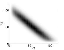
Figure 2: Probability distribution of the exclusive switch in Ex. 1.

• Example 1 (cont.).  In the exclusive switch the expected number of molecules of type $P_{1}$ and/or $P_{2}$ may become high, depending on the chosen parameters. If, for instance, $c_{1}\!=\!c_{2}\!=\!c_{9}\!=\!c_{10}\!=\!0.5$, $c_{3}\!=\!c_{4}\!=\!c_{7}\!=\!c_{8}\!=\!0.005$, $c_{5}\!=\!c_{6}\!=\!0.01$, and we start initially without any proteins, i.e. with probability one in state $\mathbf{y}=(0,0,1,0,0)$, then after 500 time units most of the probability mass is located around the states $\mathbf{x}\!=\!(92,2,0,1,0)$ and $\mathbf{x}\!=\!(2,92,0,0,1)$ (compare the plot in Fig. 2, left). Note that $x_{3}\!=\!0,x_{4}\!=\!1,x_{5}\!=\!0$ refers to the case that a molecule of type $P_{1}$ is bound to the promotor and $x_{3}\!=\!x_{4}\!=\!0,x_{5}\!=\!1$ refers to the case that a molecule of type $P_{2}$ is bound to the promotor. Since for these parameters the system is symmetric, the expected populations of $P_{1}$ and $P_{2}$ are identical. Assume that at a certain time instant, both populations reach the threshold from which on we approximate them by continuous deterministic variables (we consider the unsymmetric case later, in Section 5). The remaining discrete model then becomes finite since only $P_{1}$ and $P_{2}$ have an infinite range in the original model ($\hat{n}=2,\tilde{n}=3$). More precisely, it contains only 3 states, namely the state $\mathbf{v}_{1}$ where the promotor is free ($x_{3}\!=\!1,x_{4}\!=\!x_{5}=0$), the state $\mathbf{v}_{2}$ where $P_{1}$ is bound to the promotor ($x_{3}\!=\!0,x_{4}\!=\!1,x_{5}\!=\!0$), and the state $\mathbf{v}_{3}$ where $P_{2}$ is bound to the promotor ($x_{3}\!=\!x_{4}\!=\!0,x_{5}\!=\!1$), see also Fig. 1. For $i\in\{1,2\}$ let $W_{i}(t)$ be the population size of $P_{i}$. The differential equations which are used to approximate the conditional expectations $\Psi_{\mathbf{v}_{j}}(t+h)$, $j\in\{1,2,3\}$ are

  $$\begin{array}[]{lcl}\frac{d\phi_{\mathbf{v}_{1}}(i,t^{\prime})}{dt^{\prime}}&=&c_{i}-c_{2+i}\cdot\phi_{\mathbf{v}_{1}}(i,t^{\prime})-c_{4+i}\cdot\phi_{\mathbf{v}_{1}}(i,t^{\prime})\\[2.15277pt] \frac{d\phi_{\mathbf{v}_{2}}(i,t^{\prime})}{dt^{\prime}}&=&-c_{2+i}\cdot\phi_{\mathbf{v}_{2}}(i,t^{\prime})+(c_{7}+c_{9})\cdot(2-i)\\[2.15277pt] \frac{d\phi_{\mathbf{v}_{3}}(i,t^{\prime})}{dt^{\prime}}&=&-c_{2+i}\cdot\phi_{\mathbf{v}_{3}}(i,t^{\prime})+(c_{8}+c_{10})\cdot(i-1+)\end{array}$$

  where $\phi_{\mathbf{v}}(1,t^{\prime})$ and $\phi_{\mathbf{v}}(2,t^{\prime})$ are the elements of the vector $\Phi_{\mathbf{v}_{1}}(t^{\prime})$. Note that each of the 3 states $\mathbf{v}_{1},\mathbf{v}_{2},\mathbf{v}_{3}$ has a system of two differential equations, one for $P_{1}$ and one for $P_{2}$. The transition rates in the discrete stochastic part of the model are illustrated in Fig. 3.

  Figure 3: The discrete stochastic part of the stochastic hybrid model of Ex. 1.

  pset	purely stochastic			stochastic hybrid						purely determ.
  	ex. time	$|\mathit{Sig}|$	error	pop. thres.	ex. time	$|\mathit{Sig}|$	m1	m2	m3	ex. time	m1
  1a	11h 46min	$8\cdot 10^{5}$	$7\cdot 10^{-5}$	50	15sec	$4\cdot 10^{2}$	0.005	0.2	0.30	1sec	0.03
  				100	1min 50sec	$3\cdot 10^{3}$	0.004	0.2	0.30
  1b	7min 43sec	$5\cdot 10^{4}$	$7\cdot 10^{-7}$	50	1min 19sec	$6\cdot 10^{3}$	0.01	0.19	0.30	1sec	0.03
  				100	2min 50sec	$3\cdot 10^{4}$	0.01	0.19	0.30
  2	4h 51min	$2\cdot 10^{5}$	$4\cdot 10^{-5}$	50	25sec	$4\cdot 10^{2}$	0.06	0.08	0.09	1sec	0.45
  				100	28sec	$6\cdot 10^{2}$	0.06	0.07	0.09
  3	2min 21sec	$7\cdot 10^{5}$	$6\cdot 10^{-5}$	50	18sec	$6\cdot 10^{3}$	0.02	0.08	0.16	1sec	0.05
  				100	1min 41sec	$4\cdot 10^{4}$	0.01	0.05	0.12

  Table 2: Results for the exclusive switch example.

  Thus, after solving the differential equations above to compute $\Phi_{\mathbf{v}_{j}}(t+h)$ we obtain the vector $\Psi_{\mathbf{v}_{j}}(t+h)$ of the two conditional expectations for $P_{1}$ and $P_{2}$ from distributing $\Phi_{\mathbf{v}_{1}}(t+h)$, $\Phi_{\mathbf{v}_{2}}(t+h)$, $\Phi_{\mathbf{v}_{3}}(t+h)$ among the 3 states as defined in Eq. (17). For the parameters used in Fig. 1, left, the conditional expectations of the states $\mathbf{v}_{2}$ and $\mathbf{v}_{3}$ accurately predict the two stable regions where most of the probability mass is located. The state $\mathbf{v}_{1}$ has small probability and its conditional expectation is located between the two stable regions. It is important to point out that, for this example, a purely deterministic solution cannot detect the bistability because the deterministic model has a single steady-state [22]. Finally, we remark that in this example the number of states in the reduced discrete model is very small. If, however, populations with an infinite range but small expectations are present, we use the truncation described in Section 2 to keep the number of states small.

If at time $t$ a population, say the $i$-th population, is represented by its conditional expectations, it is possible to switch back to the original discrete stochastic treatment. This is done by adding an entry to the states $\mathbf{v}$ for the $i$-th dimension. This entry then equals $\psi_{\mathbf{v}}(i,t)$. This means that at this point we assume that the conditional probability distribution has mass one for the value $\psi_{\mathbf{v}}(i,t)$. Note that here switching back and forth between discrete stochastic and continuous deterministic representations is based on a population threshold. Thus, if the expectation of a population oscillates we may switch back and forth in each period.

5 Experimental Results

We implemented the numerical solution of the stochastic hybrid model described above in C++ as well as the fast solution of the discrete stochastic model described in Section 2. In our implementation we dynamically switch the representation of a random variable whenever it reaches a certain population threshold. We ran experiments with two different thresholds (50 and 100) on an Intel 2.5GHz Linux workstation with 8GB of RAM. In this section we present 3 examples to that we applied our algorithm, namely the exclusive switch, Goutsias’ model, and a predator-prey model. Our most complex example has 6 different chemical species and 10 reactions. We compare our results to a purely stochastic solution where switching is turned off as well as to a purely deterministic solution. For all experiments, we fixed the cutting threshold $\delta=10^{-14}$ to truncate the infinite state space as explained in Sec. 2.

model	purely stochastic			stochastic hybrid						purely determ.
	ex. time	$|\mathit{Sig}|$	error	pop. thres.	ex. time	$|\mathit{Sig}|$	m1	m2	m3	ex. time	m1
Goutsias	1h 16min	$1\cdot 10^{6}$	$4\cdot 10^{-7}$	50	8min 47sec	$1\cdot 10^{5}$	0.001	0.07	0.13	1sec	0.95
				100	48min 57sec	$6\cdot 10^{5}$	0.0001	0.0003	0.001
p.-prey	6h 6min	$5\cdot 10^{5}$	$1\cdot 10^{-7}$	50	8min 56sec	$2\cdot 10^{4}$	0.06	0.15	0.27	1sec	0.86
				100	1h 2min	$8\cdot 10^{4}$	0.04	0.11	0.23

Table 3: Results for Goutsias’ model and the predator-prey model.

Exclusive Switch. We chose different parameters for the exclusive switch in order to test whether our hybrid approach works well if

• the populations of $P_{1}$ and $P_{2}$ are large (a) or small (b),

• the model is unsymmetric (e.g. $P_{1}$ is produced at a higher rate than $P_{2}$ and degrades at a slower rate than $P_{2}$),

• the bistable form of the distribution is destroyed (i.e. promotor binding is less likely, unbinding is more likely).

The following table lists the parameter sets (psets):

$\begin{array}[]{@{\vrule\,}c@{\,\vrule\,}c@{\,\vrule\,}c@{\,\vrule\,}c@{\,\vrule\,}c@{\,\vrule\,}c@{\,\vrule\,}c@{\,\vrule\,}c@{\,\vrule\,}c@{\,\vrule\,}c@{\,\vrule\,}c@{\,\vrule}}\hline\cr\mbox{pset}&c_{1}&c_{2}&c_{3}&c_{4}&c_{5}&c_{6}&c_{7}&c_{8}&c_{9}&c_{10}\\ \hline\cr 1a&5&5&0.0005&0.0005&0.1&0.1&0.005&0.005&5&5\\ \hline\cr 1b&0.5&0.5&0.0005&0.0005&0.1&0.1&0.005&0.005&0.5&0.5\\ \hline\cr 2&5&0.5&0.0005&0.005&0.1&0.1&0.005&0.005&5&0.5\\ \hline\cr 3&0.5&0.5&0.0005&0.0005&0.01&0.01&0.1&0.1&0.5&0.5\\ \hline\cr\end{array}$

We chose a time horizon of $t=500$ for all parameter sets. Note that in the case of pset 3 the probability distribution forms a thick line in the state space (compare the plot in Fig. 2, right). We list our results in Table 2 where the first column refers to the parameter set. Column 2 to 4 list the results of a purely stochastic solution (see Section 2) where “ex. time” refers to the execution time, $|\mathit{Sig}|$ to the average size of the set of significant states and “error” refers to the amount of probability mass lost due to the truncation with threshold $\delta$, i.e. $1-\sum_{\mathbf{x}\in\mathit{Sig}}p(\mathbf{x},t)$. The columns 6-10 list the results of our stochastic hybrid approach and column 5 lists the population threshold used for switching in the representations in the stochastic hybrid model. Here, “m1”, “m2”, “m3” refer to the relative error of the first three moments of the joint probability distribution at the final time instant. For this, we compare the (approximate) solution of the hybrid model with the solution of the purely stochastic model. Since we have five species, we simply take the average relative error over all species. Note that even if a species is represented by its conditional expectations, we can approximate its first three moments by

$$\textstyle E[\mathbf{W}(t)^{i}]\approx\sum_{\mathbf{v}}\left(\Psi_{\mathbf{v}}(t)\right)^{i}\cdot r(\mathbf{v},t)$$

where the $i$-th power of the vectors are taken component-wise. Finally, in the last two columns we list the results of a purely deterministic solution as explained in Section 3. The last column refers to the average relative error of the expected populations when we compare the purely deterministic solution to the purely stochastic solution. Note that the deterministic solution of the exclusive switch yields an accurate approximation of the first moment (except for pset 2) because of the symmetry of the model. It does, however, not reveal the bistability of the distribution. As opposed to that, the hybrid solution does show this important property. For pset 1 and 3, the conditional expectations of the 3 discrete states are such that two of them match exactly the two stable regions where most of the probability mass is located (see also Example 1 in Sec. 4) . The remaining conditional expectation of the state where the promotor region is free has small probability and predicts a conditional expectation between the two stable regions. The execution time of the purely stochastic approach is high in the case of pset 1a, because the expected populations of $P_{1}$ and $P_{2}$ are high. This yields large sizes of $\mathit{Sig}$ while we iterate over time. During the hybrid solution, we switch when the populations reach the threshold and the size of $\mathit{Sig}$ drops to 3. Thus, the average number of significant states is much smaller. In the case of pset 1b, the expected populations are small and we use a deterministic representation for protein populations only during a short time interval (at the end of the time horizon). For pset 2, the accuracy of the purely deterministic solution is poor because the model is no longer symmetric. The accuracy of the hybrid solution on the other hand is independent of the symmetry of the model.

Goutsias’ Model. In [11], Goutsias defines a model for the transcription regulation of a repressor protein in bacteriophage $\lambda$. This protein is responsible for maintaining lysogeny of the $\lambda$ virus in E. coli. The model involves 6 different species and the following 10 reactions.

$\begin{array}[]{r@{: \ }l@{\,}c@{\,}l@{\hspace{2ex}}r@{: \ }l@{\,}c@{\,}l}1&\mbox{\small RNA}&\to&\mbox{\small RNA}\!+\!\mbox{\small M}\hfil\hskip 8.61108pt&6&\mbox{\small DNA.D}&\to&\mbox{\small DNA}\!+\!\mbox{\small D}\\ 2&\mbox{\small M}&\to&\emptyset\hfil\hskip 8.61108pt&7&\mbox{\small DNA.D}\!+\!\mbox{\small D}&\to&\mbox{\small DNA.2D}\\ 3&\mbox{\small DNA.D}&\to&\mbox{\small RNA}\!+\!\mbox{\small DNA.D}\hfil\hskip 8.61108pt&8&\mbox{\small DNA.2D}&\to&\mbox{\small DNA.D}\!+\!\mbox{\small D}\\ 4&\mbox{\small RNA}&\to&\emptyset\hfil\hskip 8.61108pt&9&\mbox{\small M}+\mbox{\small M}&\to&\mbox{\small D}\\ 5&\mbox{\small DNA}\!+\!\mbox{\small D}&\to&\mbox{\small DNA.D}\hfil\hskip 8.61108pt&10&\mbox{\small D}&\to&\mbox{\small M}\!+\!\mbox{\small M}\\ \end{array}$

We used the following parameters that differ from the original parameters used in [11] in that they increases the number of RNA molecules (because with the original parameters, all populations remain small).

$\begin{array}[]{@{\vrule\,}c@{\,\vrule\,}c@{\,\vrule\,}c@{\,\vrule\,}c@{\,\vrule\,}c@{\,\vrule\,}c@{\,\vrule\,}c@{\,\vrule\,}c@{\,\vrule\,}c@{\,\vrule\,}c@{\,\vrule}}\hline\cr c_{1}&c_{2}&c_{3}&c_{4}&c_{5}&c_{6}&c_{7}&c_{8}&c_{9}&c_{10}\\ \hline\cr 0.043&7\mbox{e{-4}}&71.5&\mbox{3.9e{-6}}&0.02&0.48&\mbox{2e{-4}}&\mbox{9e{-12}}&0.08&0.5\\ \hline\cr\end{array}$

Figure 4: Expected populations in Goutsias’ model.

Table 3 shows the results for the Goutsias’ model where we use the same column labels as above. We always start initially with 10 molecules of RNA, M, and D, as well as 2 DNA molecules. We choose the time horizon as $t=4$. Note that the hybrid solution as well as the purely deterministic solution are feasible for much longer time horizons. The increase of the size of the set of significant states makes the purely stochastic solution infeasible for longer time horizons. As opposed to that the memory requirements of the hybrid solution remain tractable. In Fig. 4 we plot the means of two of the six species obtained from the purely stochastic (stoch), purely deterministic (determ), and the hybrid (hyb) solution. Note that a purely deterministic solution yields very poor accuracy (relative error of the means is 95%).

Predator Prey. We apply our algorithm to the predator prey model described in [9]. It involves two species $A$ and $B$ and the reactions are $A\to 2A$, $A+B\to 2B$, and $B\to\emptyset$. The model shows sustainable periodic oscillations until eventually the population of $B$ reaches zero. We use this example to test the switching mechanism of our algorithm. We choose rate constants $c_{1}=1$, $c_{2}=0.03$, $c_{3}=1$ and start initially with 30 molecules of type $A$ and 120 molecules of type $B$. For a population threshold of 50, we start with a stochastic representation of $A$ and a deterministic representation of $B$. Then, around time $1.3$ we switch to a purely stochastic representation since the expectation of $B$ becomes less than 50. Around time $t=6.1$ we switch the representation of $A$ because $E[A(t)]>50$, etc. We present our detailed results in Table 3. Similar to Goutsias’ model, the deterministic solution has a high relative error whereas the hybrid solution yields accurate results.

6 Conclusion

We presented a stochastic hybrid model for the analysis of networks of chemical reactions. This model is based on a dynamic switching between a discrete stochastic and a continuous deterministic representation of the chemical populations. Instead of solving the underlying partial differential equation, we propose a fast numerical procedure that exploits the fact that for large populations the conditional expectations give appropriate approximations. Our experimental results substantiate the usefulness of the method. As future work we plan to include a diffusion approximation for populations of intermediate size.

References

- [1] K. Ball, T. G. Kurtz, L. Popovic, and G. Rempala. Asymptotic analysis of multiscale approximations to reaction networks. The Annals of Applied Probability, 16(4):1925–1961, 2006.
- [2] M. L. Bujorianu and J. Lygeros. Towars a general theory of stochastic hybrid systems. In Stochastic Hybrid Systems, volume 337 of Lecture Notes in Control and Information Sciences, pages 3–30. Springer, 2006.
- [3] K. Burrage, M. Hegland, F. Macnamara, and B. Sidje. A Krylov-based finite state projection algorithm for solving the chemical master equation arising in the discrete modelling of biological systems. In Proceedings of the Markov 150th Anniversary Conference, pages 21–38. Boson Books, 2006.
- [4] C. Cassandras and J. Lygeros. Stochastic hybrid systems: Research issues and areas. In Stochastic Hybrid Systems, (C.G. Cassandras, and J. Lygeros, Ed.s), pages 1–14. Taylor and Francis, 2006.
- [5] F. Didier, T. A. Henzinger, M. Mateescu, and V. Wolf. Approximation of event probabilities in noisy cellular processes. In Proc. of CMSB, volume 5688 of LNBI, page 173, 2009.
- [6] F. Didier, T. A. Henzinger, M. Mateescu, and V. Wolf. Fast adaptive uniformization of the chemical master equation. In Proc. of HIBI, pages 118–127. IEEE Computer Society, 2009.
- [7] S. Engblom. Spectral approximation of solutions to the chemical master equation. Journal of Computational and Applied Mathematics, 229(1):208 – 221, 2009.
- [8] N. Fedoroff and W. Fontana. Small numbers of big molecules. Science, 297:1129–1131, 2002.
- [9] D. T. Gillespie. Exact stochastic simulation of coupled chemical reactions. J. Phys. Chem., 81(25):2340–2361, 1977.
- [10] D. T. Gillespie. A rigorous derivation of the chemical master equation. Physica A, 188:404–425, 1992.
- [11] J. Goutsias. Quasiequilibrium approximation of fast reaction kinetics in stochastic biochemical systems. J. Chem. Phys., 122(18):184102, 2005.
- [12] E. L. Haseltine and J. B. Rawlings. Approximate simulation of coupled fast and slow reactions for chemical kinetics. J. Chem. Phys., 117:6959–6969, 2002.
- [13] M. Hegland, C. Burden, L. Santoso, S. Macnamara, and H. Booth. A solver for the stochastic master equation applied to gene regulatory networks. J. Comput. Appl. Math., 205:708–724, 2007.
- [14] A. Hellander and P. Lötstedt. Hybrid method for the chemical master equation. Journal of Computational Physics, 227, 2007.
- [15] D. Henderson, R. Boys, C. Proctor, and D. Wilkinson. Linking systems biology models to data: a stochastic kinetic model of p53 oscillations. In Handbook of Appl. Bayesian Analysis. Oxford University Press, 2009.
- [16] T. Henzinger, M. Mateescu, and V. Wolf. Sliding window abstraction for infinite Markov chains. In Proc. CAV, volume 5643 of LNCS, pages 337–352. Springer, 2009.
- [17] G. Horton, V. G. Kulkarni, D. M. Nicol, and K. S. Trivedi. Fluid stochastic Petri nets: Theory, applications, and solution techniques. European Journal of Operational Research, 105(1):184–201, 1998.
- [18] T. Jahnke. An adaptive wavelet method for the chemical master equation. SIAM J. Scientific Computing, 31(6):4373–4394, 2010.
- [19] A. Jensen. Markoff chains as an aid in the study of Markoff processes. Skandinavisk Aktuarietidskrift, 36:87–91, 1953.
- [20] N. G. v. Kampen. Stochastic Processes in Physics and Chemistry. Elsevier, 3rd edition, 2007.
- [21] T. Kurtz. Approximation of Population Processes. Society for Industrial Mathematics, 1981.
- [22] A. Loinger, A. Lipshtat, N. Q. Balaban, and O. Biham. Stochastic simulations of genetic switch systems. Phys. Rev. E, 75(2):021904, 2007.
- [23] H. H. McAdams and A. Arkin. Stochastic mechanisms in gene expression. PNAS, USA, 94:814–819, 1997.
- [24] H. H. McAdams and A. Arkin. It’s a noisy business! Trends in Genetics, 15(2):65–69, 1999.
- [25] B. Munsky and M. Khammash. The finite state projection algorithm for the solution of the chemical master equation. J. Chem. Phys., 124:044144, 2006.
- [26] P. Patel, B. Arcangioli, S. Baker, A. Bensimon, and N. Rhind. DNA replication origins fire stochastically in fission yeast. Mol. Biol. Cell, 17:308–316, 2006.
- [27] J. Paulsson. Summing up the noise in gene networks. Nature, 427(6973):415–418, 2004.
- [28] B. Philippe and R. Sidje. Transient solutions of Markov processes by Krylov subspaces. In Proc. of the 2nd International Workshop on the Numerical Solution of Markov Chains, pages 95–119. Kluwer Academic Publishers, 1995.
- [29] J. Puchalka and A. M. Kierzek. Bridging the gap between stochastic and deterministic regimes in the kinetic simulations of the biochemical reaction networks. Biophysical Journal, 86(3):1357 – 1372, 2004.
- [30] C. Rao, D. Wolf, and A. Arkin. Control, exploitation and tolerance of intracellular noise. Nature, 420(6912):231–237, 2002.
- [31] H. Salis and Y. Kaznessis. Accurate hybrid stochastic simulation of a system of coupled chemical or biochemical reactions. J. Chem. Phys., 122, 2005.
- [32] R. Sidje, K. Burrage, and S. MacNamara. Inexact uniformization method for computing transient distributions of Markov chains. SIAM J. Sci. Comput., 29(6):2562–2580, 2007.
- [33] W. J. Stewart. Introduction to the Numerical Solution of Markov Chains. Princeton University Press, 1995.
- [34] P. S. Swain, M. B. Elowitz, and E. D. Siggia. Intrinsic and extrinsic contributions to stochasticity in gene expression. PNAS, USA, 99(20):12795–12800, 2002.
- [35] A. Warmflash and A. Dinner. Signatures of combinatorial regulation in intrinsic biological noise. PNAS, 105(45):17262–17267, 2008.