2pt
Dark Energy, Anthropic Selection Effects, Entropy and Life
Chas Astro Egan
A thesis submitted for the degree of
Doctor of Philosophy
of The University of New South Wales
![[Uncaptioned image]](/html/1005.0745/assets/x1.png)
School of Physics
The University of New South Wales
Sydney NSW
Australia
28 of August, 2009
To Tonga, may your coconuts grow.
Statement of Originality
I hereby declare that this submission is my own work and to the best of my knowledge it contains no materials previously published or written by another person, or substantial proportions of material which have been accepted for the award of any other degree or diploma at UNSW or any other educational institution, except where due acknowledgement is made in the thesis. Any contribution made to the research by others, with whom I have worked at UNSW or elsewhere, is explicitly acknowledged in the thesis. I also declare that the intellectual content of this thesis is the product of my own work, except to the extent that assistance from others in the project’s design and conception or in style, presentation and linguistic expression is acknowledged.
(Signed)
(Date)
Abstract
According to the standard CDM model, the matter and dark energy densities ( and ) are only comparable for a brief time. Using the temporal distribution of terrestrial planets inferred from the cosmic star formation history, we show that the observation is expected for terrestrial-planet-bound observers under CDM, or under any model of dark energy consistent with observational constraints. Thus we remove the coincidence problem as a factor motivating dark energy models.
We compare the Sun to representative stellar samples in properties plausibly related to life. We find the Sun to be most anomalous in mass and galactic orbital eccentricity. When the properties are considered together we find that the probability of randomly selecting a star more typical than the Sun is only . Thus the observed “anomalies” are consistent with statistical noise. This contrasts with previous work suggesting anthropic explanations for the Sun’s high mass.
The long-term future of dissipative processes (such as life) depends on the continued availability of free energy to dissipate thereby increasing entropy. The entropy budget of the present observable Universe is dominated by supermassive black holes in galactic cores. Previous estimates of the total entropy in the observable Universe were between and . Using recent measurements of the supermassive black hole mass function we find the total entropy in the observable Universe to be , at least an order of magnitude higher than previous estimates. We compute the entropy in new subdominant components and report a new entropy budget of the Universe with quantified uncertainties. We evaluate upper bounds on the entropy of a comoving volume (normalized to the present observable Universe). Under the assumption that energy in matter is constant in a comoving volume, the availability of free energy is found to be finite and the future entropy in the volume is limited to a constant of order . Through this work we uncover a number of unresolved questions with implications for the ultimate fate of the Universe.
Acknowledgments
I want to thank my unofficial supervisor, Charles Lineweaver, for the years of inspiration and guidance. Charley has an enthusiasm for getting to the bottom of fundamental scientific issues which is not dissuaded by dogma or conventional disciplinary borders.
Secondly, to the Research School of Astronomy and Astrophysics at the Australian National University, thank you for generously hosting me for the majority of my candidature. Mount Stromlo is steeped in academic heritage. It is a wonderful and inspiring place to work. The drive up the mountain is always a delight.
I would like to thank my official supervisor, John Webb and others in the School of Physics at the University of New South Wales for making it possible for me to carry out my candidature remotely.
A warm gracias my most excellent academic brother Jose Robles for turning me into a mac user. It was a pleasure coding with you. To Shane, my office-mate and pepsi lover, and to Josh, the gentoo guru, to Leith my mediocre table tennis partner, to Brad for organizing all the great events, and to Dan and Grant for those mellow days at the beach, thanks for all the good times.
I am indebted to my big family at the Woden Fish Market for always making me feel close to the ocean.
Mum, Dad and Hayley, thank you for 27 years of love and support.
Finally and most importantly, Anna, my soulmate, you have given me more than it is fair to ask of anyone. Every day with you is grand no matter where we are. Thanks for supporting this dream of mine. I love you forever.
Preface
The contents of this thesis are based on research articles that I have published during the course of my PhD candidature. Although I use the first person plural throughout, all of the work presented in this thesis is my own unless explicitly stated here, or in section 1.5 of the Introduction.
-
C. H. Lineweaver & C. A. Egan, 2007, “The Cosmic Coincidence as a Temporal Selection Effect Produced by the Age Distribution of Terrestrial Planets in the Universe”, ApJ, v671, 853–860.
-
C. A. Egan & C. H. Lineweaver, 2008, “Dark Energy Dynamics Required to Solve the Cosmic Coincidence”, Phys. Rev. D., v78(8), 083528.
-
J. A. Robles, C. H. Lineweaver, D. Grether, C. Flynn, C. A. Egan, M. Pracy, J. Holmberg & E. Gardner, 2008, “A comprehensive comparison of the Sun to other stars: searching for self-selection effects”, ApJ, v684, 691–706.
-
J. A. Robles, C. A. Egan & C. H. Lineweaver, 2009, “Statistical Analysis of Solar and Stellar Properties”, Australian Space Science Conference Series: 8th Conference Proceedings NSSA Full Referreed Proceedings CD, (ed) National Space Society of Australia Ltd, edt. W. Short, conference held in Canberra, Australia September 23–25, 2008, ISBN 13: 978-0-9775740-2-5.
-
C.A. Egan & C.H. Lineweaver, 2010, “A Larger Estimate of the Entropy of the Universe”, ApJ, v710, 1825-1834.
-
C.A. Egan & C.H. Lineweaver, 2010, “The Cosmological Heat Death”, in preparation.
I have attached as appendix A a publication that is predominantly the work of my supervisor, Charles. H. Lineweaver, but to which I made minor contributions.
-
C.H. Lineweaver & C.A. Egan, 2008, “Life, gravity and the second law of thermodynamics.” Physics of Life Reviews, v5, 225–242.
Chapter 1 Introduction
I may be reckless, may be a fool,
but I get excited when I get confused.
- Fischerspooner, “The Best Revenge”
1.1 Copernicanism and Anthropic Selection
The Copernican idea, that we perceive the Universe from an entirely mediocre vantage point, is deeply embedded in the modern scientific world view. Before the influences of Copernicus, Galileo and Newton in the 16th and 17th centuries the prevalent world view was anthropocentric: we and the Earth were at the center of the Universe, and the heavenly bodies lived on spherical planes around us. The paradigm shift to a Copernican world view was ferociously resisted by theologians and philosophers, but was eventually adopted because of its ability to explain mounting physical and astronomical observations.
It is with great esteem that we remember these pioneers of modern science, who taught us that observational evidence trumps philosophical aesthetics. However, upon pedantic inspection, the Copernican idea leads to untrue predictions. For example, if we did occupy a mediocre vantage point then the density of our immediate environment would be . However the density of our actual environment is . A napkin calculation considering the density and size of collapsed objects suggest the chance of us living in an environment as dense or denser by pure chance is around in a significant signal.
There are selection effects connected with being an observer. They determine, to some degree, where and when we observe the Universe. At the cost of strict Copernicanism we must make considerations for anthropic selection as a class of observational selection effect (Dicke, 1961; Carter, 1974; Barrow and Tipler, 1986; Bostrom, 2002), and we must take the appropriate steps to remove anthropic selection effects from our data.
1.2 The Cosmic Coincidence Problem
Recent cosmological observations including observations of the cosmic microwave background temperature fluctuations, the luminosity-redshift relation from supernova light-curves and the matter power spectrum measured in the large scale structure and Lyman-Alpha forests of quasar spectra, have converged on a cosmological model which is expanding, and whose energy density is dominated by a mysterious component referred to generally as dark energy () but contains a comparable amount of matter () and some radiation (). See e.g. (Seljak et al., 2006) and references therein.
The energy in these components drives the expansion of the Universe via the Friedmann equation, and in turn responds to the expansion via their equations of state: radiation dilutes as , matter dilutes as the dark energy density remains constant (assuming that dark energy is Einstein’s cosmological constant) where is the scalefactor of the Universe (Carroll, 2004).
Since matter and dark energy dilute at different rates during cosmic expansion, these two components only have comparable densities for a brief interval during cosmic history. Thus we are faced with the “cosmic coincidence problem”: Why, just now, do the matter and dark energy densities happen to be of the same order (Weinberg, 1989; Carroll, 2001b)? Ad-hoc dynamic dark energy (DDE) models have been designed to solve the cosmic coincidence problem by arranging that the dark energy density is similar to the matter density for significant fractions of the age of the Universe.
Whether or not there is a coincidence problem depends on the range of times during which the Universe may be observed. In Chapter 2, we quantify the severity of the coincidence problem under CDM by using the temporal distribution of terrestrial planets as a basis for the probable times of observation.
In Chapter 3 we generalize this approach to quantify the severity of the coincidence problem for all models of dark energy (using a standard parameterization). The two possible outcomes of this line of investigation are both valuable. One the one hand finding a significant coincidence problem for otherwise observationally allowed dark energy models would rule them out, complementing observational constraints on dark energy. On the other hand, finding that the coincidence problem vanishes for all observationally allowed models would remove the cosmic coincidence problem as a factor motivating dark energy models.
1.3 Searching for Life Tracers Amongst the Solar Properties
If the origin and evolution of terrestrial-planet-bound observers depend on anomalous properties of the planet’s host star, then the stars that host such observers (including the Sun) are anthropically selected to have those properties.
Gonzalez (1999a, b) found that the Sun was more massive than of stars, and suggested that this may be explained if observers may develop preferentially around very massive stars. A star’s mass determines, in large part, its lifetime, luminosity, temperature and the location of the terrestrial habitable zone, all of which may influence the probability of that star hosting observers. But the statistical significance of this “anomalous” mass depends on the number of other solar properties, also plausibly related to life, from which mass was selected. Thus while Gonzalez’s proposition is plausible, it is unclear how strongly it is supported by the data.
In Chapter 4 of this thesis we compare the Sun to representative samples of stars in independent parameters plausibly related to life (including mass), with the aim of quantifying the overall typicality of the Sun and potentially identifying statistically significant anomalous properties - potential tracers of life in the Universe.
1.4 The Entropy of the Present and Future Universe
One feature that we can count on as being important to all life in the Universe is the availability of free energy. Indeed we can only be sure of this because all irreversible processes in the Universe consume free energy and contribute to the increasing total entropy of the Universe.
The current entropy of the observable Universe was estimated by Frampton et al. (2008) to be of a maximum possible value of . The current entropy of the observable Universe is dominated by the entropy in supermassive black holes at the centers of galaxies, followed distantly by the cosmic microwave background, neutrino background and other components.
If the entropy of the Universe reaches a value from which it could not be further increased, then all dissipative processes would cease. The idea that the future of the universe could end in such a state of thermodynamic equilibrium (a so-called heat death) was written about by Thomson (1852), and later revived within the context of an expanding Universe by Eddington (1931). Scientific and popular science literature over the past three decades is ambiguous about whether or not there will be a heat death, and if so, in what form.
In Chapter 5 we present an improved budget of the entropy of the observable Universe using new measurements of the supermassive black hole mass function. In Chapter 6 we compare the growing entropy of the Universe to upper bounds that have been proposed, and draw conclusions about the future heat death.
1.5 About the Papers Presented in this Thesis
Chapter 2 was published as Lineweaver and Egan (2007). The text was co-written with Charles Lineweaver, who is also to be credited for the original idea. However, the work presented in the paper is predominantly mine: details of the method, quantitative analyses, the preparation of all figures. For these reasons, and with Dr. Lineweaver’s endorsement, it has been included here verbatim.
In Chapter 4 I describe work published in Robles et al. (2008b), Robles et al. (2008a) and the erratum, Robles et al. (2008c). I was a co-author of this work, which was lead by Jose Robles, and I contributed in part to the collection of data (age; see figure 4.2), data analysis (advice on, and implementation of statistical, methods, as well as coding other parts of the analysis pipeline), interpretation and presentation of the results (contributing to figures and published articles). This chapter summarizes the main results paper, Robles et al. (2008b), in words that are my own. The figures are taken, with permission, from Robles et al. (2008b).
Chapter 6 is my own and will contribute towards an article currently in preparation, which we refer to as Egan and Lineweaver (2010b).
Appendix A has been published as Lineweaver and Egan (2008). The text, and most of the work presented in that paper is that of my supervisor. My contributions include the contribution of the preparation of Figure A.4. The paper is included in the appendix of this thesis as it is referred to several times, and motivates the work presented in Chapters 5 and 6.
Chapter 2 The Cosmic Coincidence as a Temporal Selection Effect Produced by the Age Distribution of Terrestrial Planets in the Universe
Late at night, stars shining bright
on me, down by the sea.
And when I see them in the sky
constantly I’m asking why
I was stranded here.
I wish I could be out in space.
- S.P.O.C.K, “Out in Space”
2.1 Is the Cosmic Coincidence Remarkable or Insignificant?
2.1.1 Dicke’s argument
Dirac (1937) pointed out the near equality of several large fundamental dimensionless numbers of the order . One of these large numbers varied with time since it depended on the age of the Universe. Thus there was a limited time during which this near equality would hold. Under the assumption that observers could exist at any time during the history of the Universe, this large number coincidence could not be explained in the standard cosmology. This problem motivated Dirac (1938) and Jordan (1955) to construct an ad hoc new cosmology. Alternatively, Dicke (1961) proposed that our observations of the Universe could only be made during a time interval after carbon had been produced in the Universe and before the last stars stop shining. Dicke concluded that this temporal observational selection effect – even one so loosely delimited – could explain Dirac’s large number coincidence without invoking a new cosmology.
Here, we construct a similar argument to address the cosmic coincidence: Why just now do we find ourselves in the relatively brief interval during which . The temporal constraints on observers that we present are more empirical and specific than those used in Dicke’s analysis, but the reasoning is similar. Our conclusion is also similar: a temporal observational selection effect can explain the apparent cosmic coincidence. That is, given the evolution of and in our Universe, most observers in our Universe who have emerged on terrestrial planets will find . Rather than being an unusual coincidence, it is what one should expect.
There are two distinct problems associated with the cosmological constant (Weinberg, 2000a; Garriga and Vilenkin, 2001; Steinhardt, 2003). One is the coincidence problem that we address here. The other is the smallness problem and has to do with the observed energy density of the vacuum, . Why is so small compared to the times larger value predicted by particle physics? Anthropic solutions to this problem invoke a multiverse and argue that galaxies would not form and there would be no life in a Universe, if were larger than times its observed value (Weinberg, 1987; Martel et al., 1998; Garriga and Vilenkin, 2001; Pogosian and Vilenkin, 2007). Such explanations for the smallness of do not explain the temporal coincidence between the time of our observation and the time of the near-equality of and . Here we address this temporal coincidence in our Universe, not the smallness problem in a multiverse.
2.1.2 Evolution of the Energy Densities
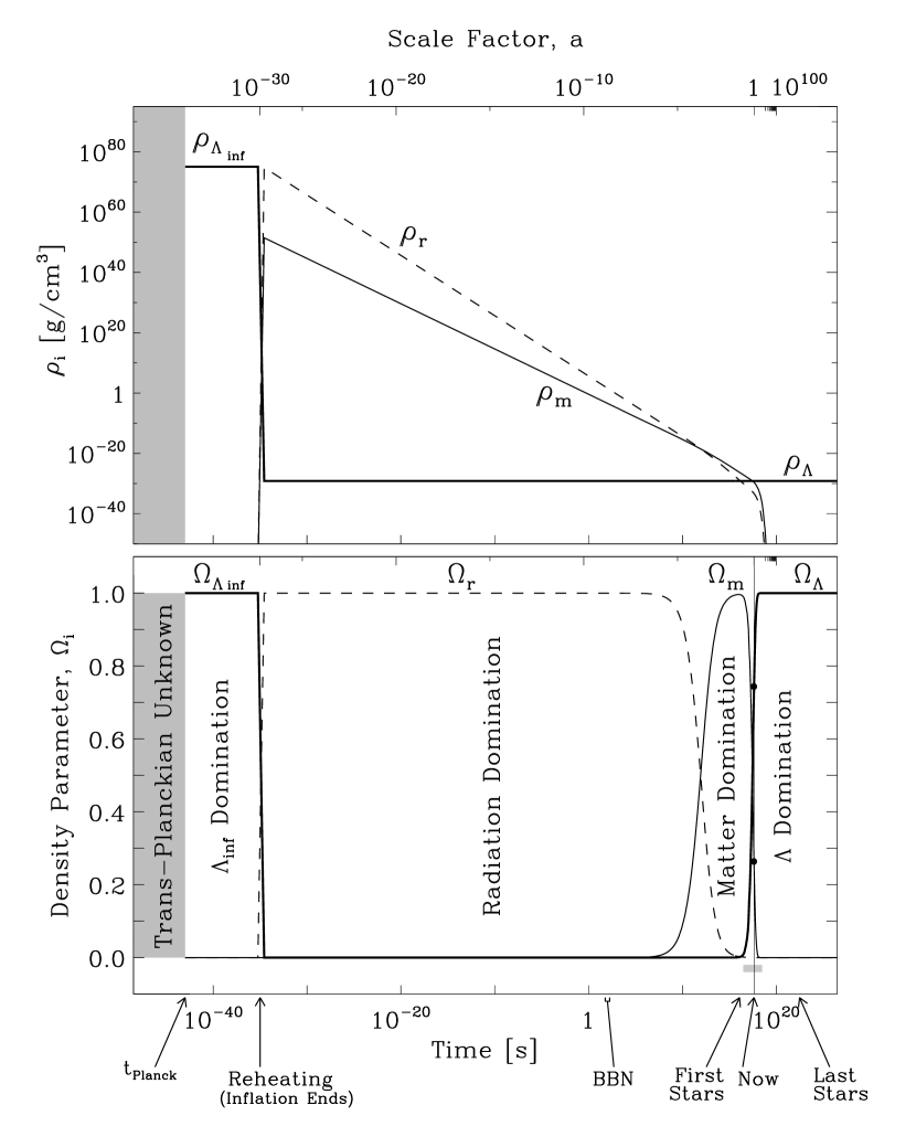
Given the currently observed values for and the energy densities , and in the Universe (Spergel et al., 2006; Seljak et al., 2006), the Friedmann equation tells us the evolution of the scale factor , and the evolution of these energy densities. These are plotted in Fig. 2.1. The history of the Universe can be divided chronologically into four distinct periods each dominated by a different form of energy: initially the false vacuum energy of inflation dominates, then radiation, then matter, and finally vacuum energy. Currently the Universe is making the transition from matter domination to vacuum energy domination. In an expanding Universe, with an initial condition , there will be some epoch in which , since is decreasing as while is a constant (see top panel of Fig. 2.1 and Appendix A). Figure 2.1 also shows that the transition from matter domination to vacuum energy domination is occurring now. When we view this transition in the context of the time evolution of the Universe (Fig. 2.2) we are presented with the cosmic coincidence problem: Why just now do we find ourselves at the relatively brief interval during which this transition happens? Carroll (2001b, a) and Dodelson et al. (2000) find this coincidence to be a remarkable result that is crucial to understand. The cosmic coincidence problem is often regarded as an important unsolved problem whose solution may help unravel the nature of dark energy (Turner 2001; Carroll 2001a). The coincidence problem is one of the main motivations for the tracker potentials of quintessence models (Caldwell et al., 1998; Steinhardt et al., 1999; Zlatev et al., 1999; Wang et al., 2000; Dodelson et al., 2000; Armendariz-Picon et al., 2001; Guo and Zhang, 2005). In these models the cosmological constant is replaced by a more generic form of dark energy in which and are in near-equality for extended periods of time. It is not clear that these models successfully explain the coincidence without fine-tuning (see Weinberg 2000a; Bludman 2004).
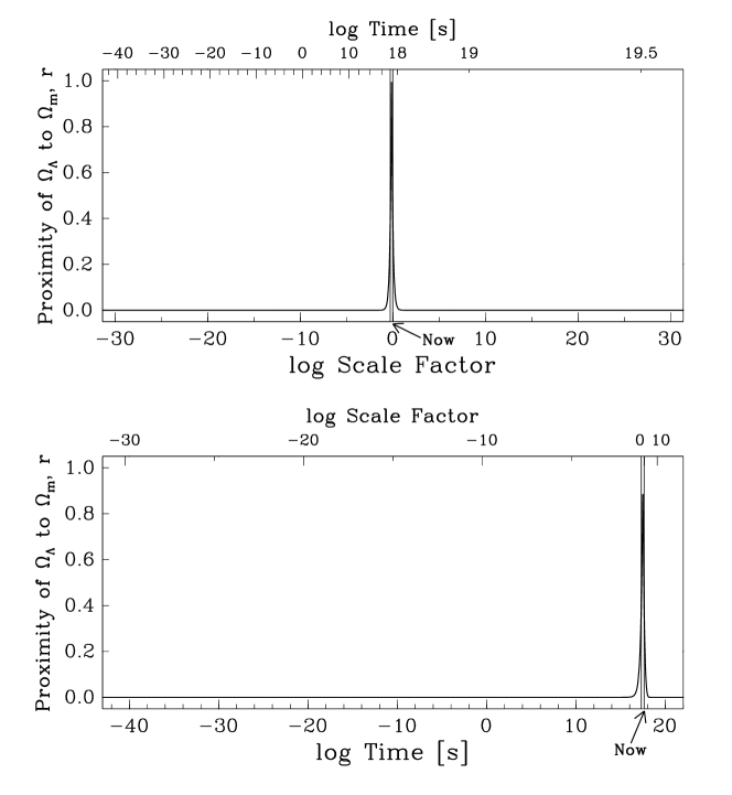
The interpretation of the observation as a remarkable coincidence in need of explanation depends on some assumptions that we quantify to determine how surprising this apparent coincidence is. We begin this quantification by introducing a time-dependent proximity parameter,
| (2.1) |
which is equal to one when and is close to zero when or . The current value is . In Figure 2.2 we plot as a function of log(scale factor) in the upper panel and as a function of log(time) in the lower panel. These logarithmic axes allow a large dynamic range that makes our existence at a time when , appear to be an unlikely coincidence. This appearance depends on the implicit assumption that we could make cosmological observations at any time with equal likelihood. More specifically, the implicit assumption is that the a priori probability distribution , of the times we could have made our observations, is uniform in log , or log , over the interval shown.
Our ability to quantify the significance of the coincidence depends on whether we assume that is uniform in time, log(time), scale factor or log(scale factor). That is, our result depends on whether we assume: , , or . These are the most common possibilities, but there are others. For a discussion of the relative merits of log and linear time scales and implicit uniform priors see Section 2.3.3 and Jaynes (1968).
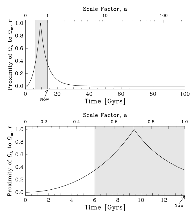
In Fig. 2.3 we plot on an axis linear in time where the implicit assumption is that the a priori probability distribution of our existence is uniform in over the intervals Gyr (top panel) and Gyr (bottom panel). The bottom panel shows that the observation could have been made anytime during the past 7.8 Gyr. Thus, our current observation that , does not appear to be a remarkable coincidence. Whether this most recent 7.8 Gyr period is seen as “brief” (in which case there is an unlikely coincidence in need of explanation) or “long” (in which case there is no coincidence to explain) depends on whether we view the issue in log time (Fig. 2.2) or linear time (Fig. 2.3).
A large dynamic range is necessary to present the fundamental changes that occurred in the very early Universe, e.g., the transitions at the Planck time, inflation, baryogenesis, nucleosynthesis, recombination and the formation of the first stars. Thus a logarithmic time axis is often preferred by early Universe cosmologists because it seems obvious, from the point of view of fundamental physics, that the cosmological clock ticks logarithmically. This defensible view and the associated logarithmic axis gives the impression that there is a coincidence in need of an explanation. The linear time axis gives a somewhat different impression. Evidently, deciding whether a coincidence is of some significance or only an accident is not easy (Peebles and Vilenkin, 1999). We conclude that although the importance of the cosmic coincidence problem is subjective, it is important enough to merit the analysis we perform here.
The interpretation of the observation as a coincidence in need of explanation depends on the a priori (not necessarily uniform) probability distribution of our existence. That is, it depends on when cosmological observers can exist. We propose that the cosmic coincidence problem can be more constructively evaluated by replacing these uninformed uniform priors with the more realistic assumption that observers capable of measuring cosmological parameters are dependent on the emergence of high density regions of the Universe called terrestrial planets, which require non-trivial amounts of time to form – and that once these planets are in place, the observers themselves require non-trivial amounts of time to evolve.
In this paper we use the age distribution of terrestrial planets estimated by Lineweaver (2001) to constrain when in the history of the Universe, observers on terrestrial planets can exist. In Section 2.2, we briefly describe this age distribution (Fig. 2.4) and show how it limits the existence of such observers to an interval in which (Fig. 2.5). Using this age distribution as a temporal selection function, we compute the probability of an observer on a terrestrial planet observing (Fig. 2.6). In Section 2.3 we discuss the robustness of our result and find (Fig. 2.7) that this result is relatively robust if the time it takes an observer to evolve on a terrestrial planet is less than Gyr. In Section 2.4 we discuss and summarize our results, and compare it to previous work to resolve the cosmic coincidence problem (Garriga and Vilenkin, 2000; Bludman and Roos, 2001).
2.2 How We Compute the Probability of Observing
2.2.1 The Age Distribution of Terrestrial Planets and New Observers
The mass histogram of detected extrasolar planets peaks at low masses: , suggesting that low mass planets are abundant (Lineweaver and Grether, 2003). Terrestrial planet formation may be a common feature of star formation (Wetherill 1996; Chyba 1999; Ida and Lin 2005). Whether terrestrial planets are common or rare, they will have an age distribution proportional to the star formation rate – modified by the fact that in the first billion years of star formation, metallicities are so low that the material for terrestrial planet formation will not be readily available. Using these considerations, Lineweaver (2001) estimated the age distribution of terrestrial planets – how many Earths are produced by the Universe per year, per (Figure 2.4). If life emerges rapidly on terrestrial planets (Lineweaver and Davis, 2002) then this age distribution is the age distribution of biogenesis in the Universe. However, we are not just interested in any life; we would like to know the distribution in time of when independent observers first emerge and are able to measure and , as we are able to do now. If life originates and evolves preferentially on terrestrial planets, then the Lineweaver (2001) estimate of the age distribution of terrestrial planets is an a priori input which can guide our expectations of when we (as members of a hypothetical group of terrestrial-planet-bound observers) could have been present in the Universe. It takes time (if it happens at all) for life to emerge on a new terrestrial planet and evolve into cosmologists who can observe and . Therefore, to obtain the age distribution of new independent observers able to measure the composition of the Universe for the first time, we need to shift the age distribution of terrestrial planets by some characteristic time, required for observers to evolve. On Earth, it took Gyr for this to happen. Whether this is characteristic of life elsewhere in the Universe is uncertain (Carter 1983; Lineweaver and Davis 2003). For our initial analysis we use Gyr as a nominal time to evolve observers. In Section 2.3.1 we allow to vary from 0-12 Gyr to see how sensitive our result is to these variations. Fig. 2.4 shows the age distribution of terrestrial planet formation in the Universe shifted by Gyr. This curve, labeled “” is a crude prior for the temporal selection effect of when independent observers can first measure . Thus, if the evolution of biological equipment capable of doing cosmology takes about Gyr, the “” in Fig. 2.4 shows the age distribution of the first cosmologists on terrestrial planets able to look at the Universe and determine the overall energy budget, just as we have recently been able to do.
2.2.2 The Probability of Observing .
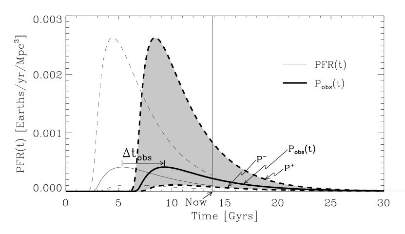
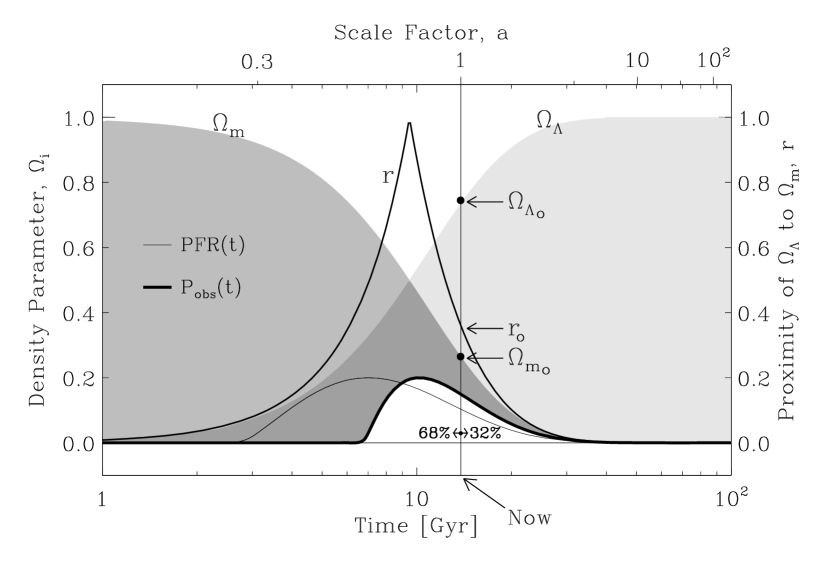
In Fig. 2.5 we zoom into the portion of Fig. 2.1 containing the relatively narrow window of time in which . We plot to show where and we also plot the age distribution of planets and the age distribution of recently emerged cosmologists from Fig. 2.4. The white area under the thick curve provides an estimate of the time distribution of new observers in the Universe. We interpret as the probability distribution of the times at which new, independent observers are able to measure for the first time.
Lineweaver (2001) estimated that the Earth is relatively young compared to other terrestrial planets in the Universe. It follows under the simple assumptions of our analysis that most terrestrial-planet-bound observers will emerge earlier than we have. We compute the fraction of observers who have emerged earlier than we have,
| (2.2) |
and find that emerge earlier while emerge later. These numbers are indicated in Fig. 2.5.
2.2.3 Converting to
We have an estimate of the distribution in time of observers, , and we have the proximity parameter . We can then convert these to a probability , of observed values of . That is, we change variables and convert the dependent probability to an dependent probability: . We want the probability distribution of the values first observed by new observers in the Universe. Let the probability of observing in the interval be . This is equal to the probability of observing in the interval , which is
Thus,
| (2.3) |
or equivalently
| (2.4) |
where is the temporally shifted age distribution of terrestrial planets and is the slope of . Both are shown in Fig. 2.5. The distribution is shown in Fig. 2.6 along with the upper and lower confidence limits on obtained by inserting the upper and lower confidence limits of (denoted “” and “” in Fig. 2.4), into Eq. 2.4 in place of .
The probability of observing is,
| (2.5) |
where is the time in the past when was equal to its present value, i.e., . We have Gyr and Gyr (see bottom panel of Fig. 2.3). This integral is shown graphically in Fig. 2.6 as the hatched area underneath the “” curve, between and . We interpret this as follows: of all observers that have emerged on terrestrial planets, 68% will emerge when and thus will find . The from Eq. 2.2 is only the same as the from Eq. 2.5 because all observers who emerge earlier than we did, did so more recently than 7.8 billion years ago and thus, observe (Fig. 2.5).
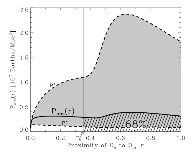
We obtain estimates of the uncertainty on this estimate by computing analogous integrals underneath the curves labeled and in Fig. 2.6. These yield and respectively. Thus, under the assumptions made here, of the observers in the Universe will find and even closer to each other than we do. This suggests that a temporal selection effect due to the constraints on the emergence of observers on terrestrial planets provides a plausible solution to the cosmic coincidence problem. If observers in our Universe evolve predominantly on Earth-like planets (see the “principle of mediocrity” in Vilenkin (1995b)), we should not be surprised to find ourselves on an Earth-like planet and we should not be surprised to find .
2.3 How Robust is this Result?
2.3.1 Dependence on the timescale for the evolution of observers
A necessary delay, required for the biological evolution of observing equipment – e.g. brains, eyes, telescopes, makes the observation of recent biogenesis unobservable (Lineweaver and Davis, 2002, 2003). That is, no observer in the Universe can wake up to observerhood and find that their planet is only a few hours old. Thus, the timescale for the evolution of observers, .
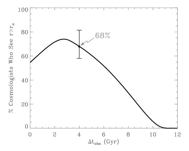
Our result was calculated under the assumption that evolution from a new terrestrial planet to an observer takes Gyr. To determine how robust our result is to variations in , we perform the analysis of Sec. 2.2 for Gyr. The results are shown in Fig. 2.7. Our result is the data point plotted at Gyr. If life takes Gyr to evolve to observerhood, once a terrestrial planet is in place, and of new cosmologists would observe an value larger than the that we actually observe today. If observers typically take twice as long as we did to evolve ( Gyr), there is still a large chance () of observing . If Gyr, in Fig. 2.5 peaks substantially after peaks, and the percentage of cosmologists who see , is close to zero (Eq. 2.5). Thus, if the characteristic time it takes for life to emerge and evolve into cosmologists is Gyr, our analysis provides a plausible solution to the cosmic coincidence problem.
The Sun is more massive than of all stars. Therefore of stars live longer than the Gyr main sequence lifetime of the Sun. This is mildly anomalous and it is plausible that the Sun’s mass has been anthropically selected. For example, perhaps stars as massive as the Sun are needed to provide the UV photons to jump start and energize the molecular evolution that leads to life. If so, then Gyr is a rough upper limit to the amount of time a terrestrial planet with simple life has to produce observers. Even if the characteristic time for life to evolve into observers is much longer than Gyr, as concluded by Carter (1983), this UV requirement that life-hosting stars have main sequence lifetimes Gyr would lead to the extinction of most extraterrestrial life before it can evolve into observers. This would lead to observers waking to observerhood to find the age of their planet to be a large fraction of the main sequence lifetime of their star; the time they took to evolve would satisfy Gyr, and they would observe that and that other observers are very rare. Such is our situation.
If we assume that we are typical observers (Vilenkin, 1995a, b, 1996a, 1996b) and that the coincidence problem must be resolved by an observer selection effect (Bostrom, 2002), then we can conclude that the typical time it takes observers to evolve on terrestrial planets is less than Gyr ( Gyr).
2.3.2 Dependence on the age distribution of terrestrial planets
The used here (Fig. 2.5) is based on the star formation rate (SFR) computed in Lineweaver (2001). There is general agreement that the SFR has been declining since redshifts . Current debate centers around whether that decline has only been since or whether the SFR has been declining from a much higher redshift (Lanzetta et al. 2002; Hopkins 2006; Nagamine et al. 2006; Thompson et al. 2006). Since Lineweaver (2001) assumed a relatively high value for the SFR at redshifts above 2, this led to a relatively high estimate of the metallicity of the Universe at , which corresponds to a relatively short delay ( Gyr) between the big bang and the first terrestrial planets. For the purposes of this analysis, the early-SFR-dependent uncertainty in the Gyr delay is degenerate with, but much smaller than, the uncertainty of . Thus the variations of discussed above subsume the SFR-dependent uncertainty in .
2.3.3 Dependence on Measure
In Figs. 2.2 & 2.3 we illustrated how the importance of the cosmic coincidence depends on the range over which one assumes that the observation of could have occurred. This involved choosing the range shown on the x axis in Figs. 2.2 & 2.3. We also showed how the apparent significance of the coincidence depended on how one expressed that range, i.e., logarithmic in Fig. 2.2 and linear in Fig. 2.3. The coincidence seems most compelling when is the largest and the problem is presented on a logarithmic axis. This dependence is a specific example of a “measure” problem (Aguirre and Tegmark 2005; Aguirre et al. 2007).
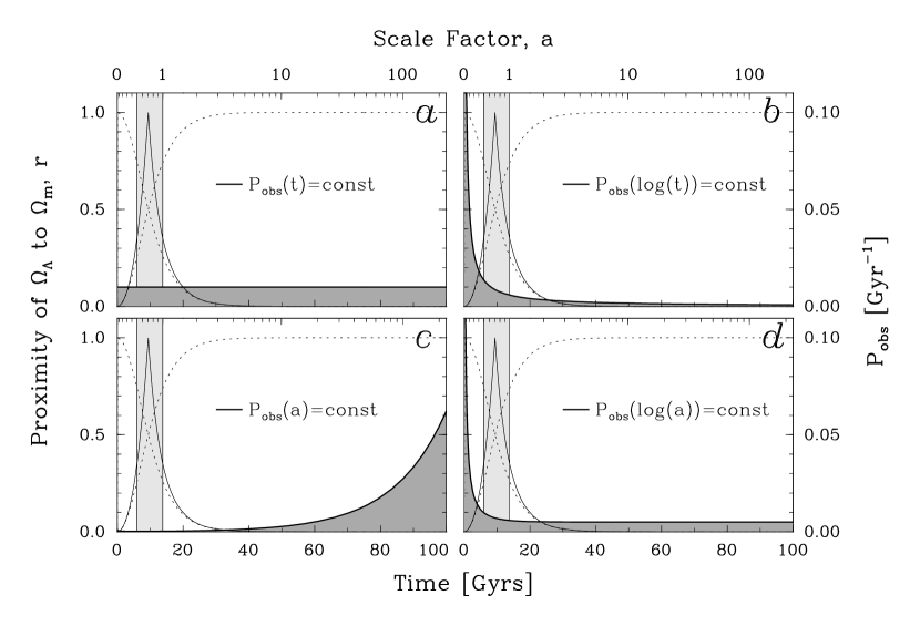
The measure problem is illustrated in Fig. 2.8, where we plot four different uniform distributions of observers on a linear time axis. In Panel a) constant. That is, we assume that observers could find themselves anywhere between yr and Gyr after the big bang, with uniform probability (dark grey). In b), we make the different assumption that observers are distributed uniformly in log(t) over the same range in time. This means for example that the probability of finding yourself between 0.1 and 1 Gyr is the same as between 1 and 10 Gyr. We plot this as a function of linear time and find that the distribution of observers (dark grey) is highest towards earlier times.
To quantify and explore these dependencies further, in Table 2.2, we take the duration when (call this interval ) and divide it by various larger ranges (a range of time or scale factor). Thus, when the probability is , there is a low probability that one would find oneself in the interval and the cosmic coincidence is compelling. However, when the coincidence is not significant.
In the four panels a,b,c and d of Fig. 2.8 the probability of us observing (finding ourselves in the light grey area) is respectively and . These values are given in the first row of Table 2.2 along with analogous values when 11 other ranges for are considered. Probabilities corresponding to the four panels of Figs. 2.2 & 2.3 are shown in bold in Table 2.2. Our conclusion is that this simple ratio method of measuring the significance of a coincidence yields results that can vary by many orders of magnitude depending on the range () and measure (e.g. linear or logarithmic) chosen. The use of the non-uniform shown in Fig. 2.4 is not subject to these ambiguities in the choice of range and measure.
2.4 Discussion & Summary
Anthropic arguments to resolve the coincidence problem include Garriga and Vilenkin (2000) and Bludman and Roos (2001). Both use a semi-analytical formalism (Gunn and Gott 1972; Press and Schechter 1974; Martel et al. 1998) to compute the number density of objects that collapse into large galaxies. This is then used as a measure of the number density of intelligent observers. Our work complements these semi-analytic models by using observations of the star formation rate to constrain the possible times of observation. Our work also extends this previous work by including the effect of , the time it takes observers to evolve on terrestrial planets. This inclusion puts an important limit on the validity of anthropic solutions to the coincidence problem.
Garriga and Vilenkin (2000) is probably the work most similar to ours. They take as a random variable in a multiverse model with a prior probability distribution. For a wide range of (prescribed by a prior based on inflation theory) they find approximate equality between the time of galaxy formation , the time when starts to dominate the energy density of the Universe and now . That is, they find that, within one order of magnitude, . Their analysis is more generic but approximate in that it addresses the coincidence for a variety of values of to an order of magnitude precision. Our analysis is more specific and empirical in that we condition on our Universe and use the Lineweaver (2001) star-formation-rate-based estimate of the age distribution of terrestrial planets to reach our main result ().
To compare our result to that of Garriga and Vilenkin (2000), we limit their analysis to the observed in our Universe () and differentiate their cumulative number of galaxies which have assembled up to a given time (their Eq. 9). We find a broad time-dependent distribution for galaxy formation which is the analog of our more empirical and narrower (by a factor of 2 or 3) .
We have made the most specific anthropic explanation of the cosmic coincidence using the age distribution of terrestrial planets in our Universe and found this explanation fairly robust to the largely uncertain time it takes observers to evolve. Our main result is an understanding of the cosmic coincidence as a temporal selection effect if observers emerge preferentially on terrestrial planets in a characteristic time Gyr. Under these plausible conditions, we, and any observers in the Universe who have evolved on terrestrial planets, should not be surprised to find .
Acknowledgements
We would like to thank Paul Francis and Charles Jenkins for helpful discussions. CE acknowledges a UNSW
School of Physics post graduate fellowship.
Appendix A: Evolution of Densities
Recent cosmological observations have led to the new standard CDM model in which the density parameters of radiation, matter and vacuum energy are currently observed to be , and respectively and Hubble’s constant is (Spergel et al., 2006; Seljak et al., 2006).
The energy densities in relativistic particles (“radiation” i.e., photons, neutrinos, hot dark matter), non-relativistic particles (“matter” i.e., baryons,cold dark matter) and in vacuum energy scale differently (Peacock, 1999),
| (2.6) |
Where the different equations of state are, where , and (Linder, 1997). That is, as the Universe expands, these different forms of energy density dilute at different rates.
| (2.7) | |||||
| (2.8) | |||||
| (2.9) |
Given the currently observed values for , and , the Friedmann equation for a standard flat cosmology tells us the evolution of the scale factor of the Universe, and the history of the energy densities:
| (2.10) | |||||
| (2.11) | |||||
| (2.12) |
where we have and . The upper panel of Fig. 2.1 illustrates these different dependencies on scale factor and time in terms of densities while the lower panel shows the corresponding normalized density parameters. A false vacuum energy is assumed between the Planck scale and the GUT scale. In constructing this density plot and setting a value for we have used the constraint that at the GUT scale, all the energy densities add up to which remains constant at earlier times.
Appendix B: Tables
| Event | Symbol | Time after Big Bang | |
|---|---|---|---|
| seconds | Gyr | ||
| Planck time, beginning of time | |||
| end of inflation, reheating, origin of matter, thermalization | |||
| energy scale of Grand Unification Theories (GUT) | |||
| matter-anti-matter annihilation, baryogenesis | |||
| electromagnetic and weak nuclear forces diverge | |||
| light atomic nuclei produced | |||
| radiation-matter equality1 | |||
| recombination1 (first chemistry) | |||
| first thermal disequilibrium | |||
| first stars, Pop III, reionization1 | |||
| first terrestrial planets2 | |||
| last time had same value as today | |||
| formation of the Sun, Earth3 | , | ||
| matter- equality1 | |||
| now | |||
| last stars die4 | |||
| protons decay4 | |||
| super massive black holes consume matter4 | |||
| maximum entropy (no gradients to drive life)4 | |||
(1) Spergel et al. 2006, http://map.gsfc.nasa.gov/
(2) Lineweaver 2001
(3) Allègre et al. 1995
(4) Adams and Laughlin 1997
| Range | [%] | ||||
|---|---|---|---|---|---|
| Gyr b | |||||
a See Table 1 for the times corresponding to columns 1 and 2.
b The four values in the top row correspond to Fig. 2.8.
c The two values shown in bold in the column correspond to the two panels of Fig. 2.3.
d These values correspond to the two panels of Fig.2.2.
Chapter 3 Dark Energy Dynamics Required to Solve the Cosmic Coincidence
Tonight I have a date on Mars.
Tonight I’m gonna get real far.
I’ll be leaving Earth behind me.
- Encounter, “Date on Mars”
3.1 Introduction
In 1998, using supernovae Ia as standard candles, Riess et al. (1998) and Perlmutter et al. (1999) revealed a recent and continuing epoch of cosmic acceleration - strong evidence that Einstein’s cosmological constant , or something else with comparable negative pressure , currently dominates the energy density of the universe (Lineweaver, 1998). is usually interpreted as the energy of zero-point quantum fluctuations in the vacuum (Zel’Dovich, 1967; Durrer and Maartens, 2007) with a constant equation of state . This necessary additional energy component, construed as or otherwise, has become generically known as “dark energy” (DE).
A plethora of observations have been used to constrain the free parameters of the new standard cosmological model, CDM , in which does play the role of the dark energy. Hinshaw et al. Hinshaw (2006) find that the universe is expanding at a rate of ; that it is spatially flat and therefore critically dense (); and that the total density is comprised of contributions from vacuum energy (), cold dark matter (CDM; ), baryonic matter () and radiation (). Henceforth we will assume that the universe is flat () as predicted by inflation and supported by observations.
Two problems have been influential in moulding ideas about dark energy, specifically in driving interest in alternatives to CDM . The first of these problems is concerned with the smallness of the dark energy density (Zel’Dovich, 1967; Weinberg, 1989; Cohn, 1998). Despite representing more than of the total energy of the universe, the current dark energy density is orders of magnitude smaller than energy scales at the end of inflation (or orders of magnitude smaller than energy scales at the end of inflation if this occurred at the GUT rather than Planck scale) (Weinberg, 1989). Dark energy candidates are thus challenged to explain why the observed DE density is so small. The standard idea, that the dark energy is the energy of zero-point quantum fluctuations in the true vacuum, seems to offer no solution to this problem.
The second cosmological constant problem Weinberg (2000b); Carroll (2001a); Steinhardt (2003) is concerned with the near coincidence between the current cosmological matter density () and the dark energy density (). In the standard CDM model, the cosmological window during which these components have comparable density is short (just e-folds of the cosmological scalefactor ) since matter density dilutes as while vacuum density is constant (Lineweaver and Egan, 2007). Thus, even if one explains why the DE density is much less than the Planck density (the smallness problem) one must explain why we happen to live during the time when .
The likelihood of this coincidence depends on the range of times during which we suppose we might have lived. In works addressing the smallness problem, Weinberg (1987, 1989, 2000a) considered a multiverse consisting of a large number of big bangs, each with a different value of . There he asked, suppose that we could have arisen in any one of these universes; What value of should we expect our universe to have? While Weinberg supposed we could have arisen in another universe, we are simply supposing that we could have arisen in another time. We ask, what time , and corresponding densities and should we expect to observe? Weinberg’s key realization was that not every universe was equally probable: those with smaller contain more Milky-Way-like galaxies and are therefore more hospitable (Weinberg, 1987, 1989). Subsequently, he, and other authors used the relative number of Milky-Way-like galaxies to estimate the distribution of observers as a function of , and determined that our value of was indeed likely (Efstathiou, 1995; Martel et al., 1998; Pogosian and Vilenkin, 2007). Our value of could have been found to be unlikely and this would have ruled out the type of multiverse being considered. Here we apply the same reasoning to the cosmic coincidence problem. Our observerhood could not have happened at any time with equal probability (Lineweaver and Egan, 2007). By estimating the temporal distribution of observers we can determine whether the observation of was likely. If we find to be unlikely while considering a particular DE model, that will enable us to rule out that DE model.
In a previous paper (Lineweaver and Egan, 2007), we tested CDM in this way and found that is expected. In the present paper we apply this test to dynamic dark energy models to see what dynamics is required to solve the coincidence problem when the temporal distribution of observers is being considered.
The smallness of the dark energy density has been anthropically explained in multiverse models with the argument that in universes with much larger DE components, DE driven acceleration starts earlier and precludes the formation of galaxies and large scale structure. Such universes are probably devoid of observers (Weinberg, 1987; Martel et al., 1998; Pogosian and Vilenkin, 2007). A solution to the coincidence problem in this scenario was outlined by Garriga et al. (1999) who showed that if is low enough to allow galaxies to form, then observers in those galaxies will observe .
To quantify the time-dependent proximity of and , we define a proximity parameter,
| (3.1) |
which ranges from , when many orders of magnitude separate the two densities, to , when the two densities are equal. The presently observed value of this parameter is . In terms of , the coincidence problem is as follows. If we naively presume that the time of our observation has been drawn from a distribution of times spanning many decades of cosmic scalefactor, we find that the expected proximity parameter is . In the top panel of Fig. 3.1 we use a naive distribution for that is constant in to illustrate how observing as large as seems unexpected.
In Lineweaver and Egan (2007) we showed how the apparent severity of the coincidence problem strongly depends upon the distribution from which is hypothesized to have been drawn. Naive priors for , such as the one illustrated in the top panel of Fig. 3.1, lead to naive conclusions. Following the reasoning of Weinberg (1987, 1989, 2000a) we interpret as the temporal distribution of observers. The temporal and spatial distribution of observers has been estimated using large () galaxies (Weinberg, 1987; Efstathiou, 1995; Martel et al., 1998; Garriga et al., 1999) and terrestrial planets (Lineweaver and Egan, 2007) as tracers. The top panel of Fig. 3.1 shows the temporal distribution of observers from Lineweaver and Egan (2007).
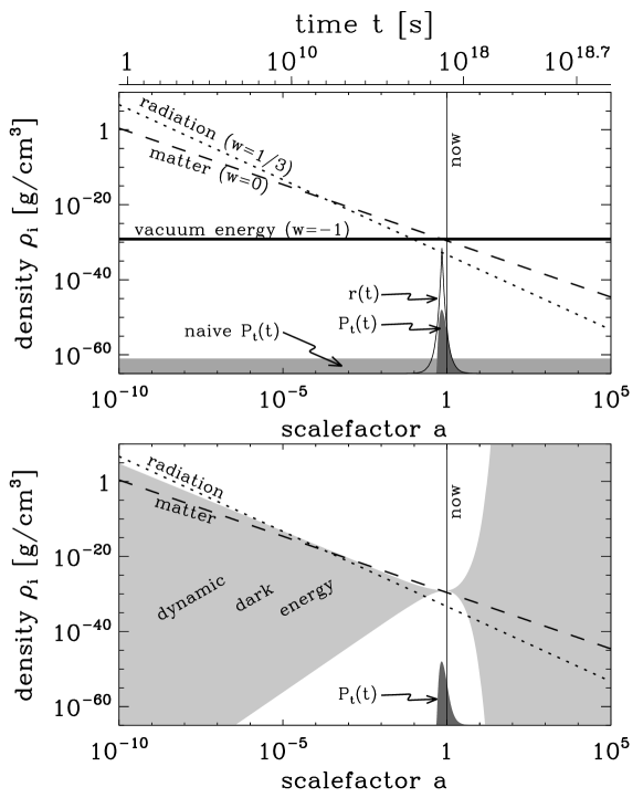
A possible extension of the concordance cosmological model that may explain the observed smallness of is the generalization of dark energy candidates to include dynamic dark energy (DDE) models such as quintessence, phantom dark energy, k-essence and Chaplygin gas. In these models the dark energy is treated as a new matter field which is approximately homogenous, and evolves as the universe expands. DDE evolution offers a mechanism for the decay of from the expected Planck scales ( g/cm3) in the early universe ( s) to the small value we observe today ( g/cm3). The light grey shade in the bottom panel of Fig. 3.1 represents contemporary observational constraints on the DDE density history. Many DDE models are designed to solve the coincidence problem by having for a large fraction of the history/future of the universe (Amendola, 2000a; Dodelson et al., 2000; Sahni and Wang, 2000; Chimento et al., 2000; Zimdahl et al., 2001; Sahni, 2002; Chimento et al., 2003; Ahmed et al., 2004; França and Rosenfeld, 2004; Mbonye, 2004; del Campo et al., 2005; Guo and Zhang, 2005; Olivares et al., 2005; Pavón and Zimdahl, 2005; Scherrer, 2005; Zhang, 2005; del Campo et al., 2006; França, 2006; Feng et al., 2006; Nojiri and Odintsov, 2006; Amendola et al., 2006, 2007; Olivares et al., 2007; Sassi and Bonometto, 2007). With for extended or repeated periods the hope is to ensure that is expected.
Our main goal in this paper is to take into account the temporal distribution of observers to determine when, and for how long, a DDE model must have in order to solve the coincidence problem? Specifically, we extend the work of Lineweaver and Egan (2007) to find out for which cosmologies (in addition to CDM ) the coincidence problem is solved when the temporal distribution of observers is considered. In doing this we answer the question, Does a dark energy model fitting contemporary constraints on the density and the equation of state parameters, necessarily solve the cosmic coincidence? Both positive and negative answers have interesting consequences. An answer in the affirmative will simplify considerations that go into DDE modeling: any DDE model in agreement with current cosmological constraints has for a significant fraction of observers. An answer in the negative would yield a new opportunity to constrain the DE equation of state parameters more strongly than contemporary cosmological surveys.
A different coincidence problem arises when the time of observation is conditioned on and the parameters of a model are allowed to slide. The tuning of parameters and the necessity to include ad-hoc physics are large problems for many current dark energy models. This paper does not address such issues, and the interested reader is referred to Hebecker and Wetterich (2001), Bludman (2004) and Linder (2006b). In the coincidence problem addressed here we let the time of observation vary to see if is unlikely according to the model.
In Section 3.2 we present several examples of DDE models used to solve the coincidence problem. An overview of observational constraints on DDE is given in Section 3.3. In Section 3.4 we estimate the temporal distribution of observers. Our main analysis is presented in Section 3.5. Our main result - that the coincidence problem is solved for all DDE models fitting observational constraints - is illustrated in Fig. 3.7. Finally, in Section 3.6, we end with a discussion of our results, their implications and potential caveats.
3.2 Dynamic Dark Energy Models in the Face of the Cosmic Coincidence
Though it is beyond the scope of this article to provide a complete review of DDE (see Copeland et al. (2006); Szydłowski et al. (2006)), here we give a few representative examples in order to set the context and motivation of our work. Fig. 3.2 illustrates density histories typical of tracker quintessence, tracking oscillating energy, interacting quintessence, phantom dark energy, k-essence, and Chaplygin gas. They are discussed in turn below.

3.2.1 Quintessence
In quintessence models the dark energy is interpreted as a homogenous scalar field with Lagrangian density (Özer and Taha, 1987; Ratra and Peebles, 1988; Ferreira and Joyce, 1998; Caldwell et al., 1998; Steinhardt et al., 1999; Zlatev et al., 1999; Dalal et al., 2001). The evolution of the quintessence field and of the cosmos depends on the postulated potential of the field and on any postulated interactions. In general, quintessence has a time-varying equation of state . Since the kinetic term cannot be negative, the equation of state is restricted to values . Moreover, if the potential is non-negative then is also restricted to values .
If the quintessence field only interacts gravitationally then energy density evolves as and the restrictions mean decays (but never faster than ) or remains constant (but never increases).
Tracker Quintessence
Particular choices for lead to interesting attractor solutions which can be exploited to make scale (“track”) sub-dominantly with .
The DE can be forced to transit to a -like () state at any time by fine-tuning . In the -like state overtakes and dominates the recent and future energy density of the universe. We illustrate tracker quintessence in Fig. 3.2 using a power law potential (panel b) (Ratra and Peebles, 1988; Caldwell et al., 1998; Zlatev et al., 1999) and an exponential potential (panel c) (Dodelson et al., 2000).
The tracker paths are attractor solutions of the equations governing the evolution of the field. If the tracker quintessence field is initially endowed with a density off the tracker path (e.g. an equipartition of the energy available at reheating) its density quickly approaches and joins the tracker solution.
Oscillating Dark Energy
Dodelson et al. (2000) explored a quintessence potential with oscillatory perturbations . They refer to models of this type as tracking oscillating energy. Without the perturbations (setting ) this potential causes exact tracker behaviour: the quintessence energy decays as and never dominates. With the perturbations the quintessence energy density oscillates about as it decays (Fig. 3.2d). The quintessence energy dominates on multiple occasions and its equation of state varies continuously between positive and negative values. One of the main motivations for tracking oscillating energy is to solve the coincidence problem by ensuring that or at many times in the past or future.
Interacting Quintessence
Non-gravitational interactions between the quintessence field and matter fields might allow energy to transfer between these components. Such interactions are not forbidden by any known symmetry Amendola (2000b). The primary motivation for the exploration of interacting dark energy models is to solve the coincidence problem. In these models the present matter/dark energy density proximity may be constant (Amendola, 2000a; Zimdahl et al., 2001; Amendola and Quercellini, 2003; França and Rosenfeld, 2004; Guo and Zhang, 2005; Olivares et al., 2005; Pavón and Zimdahl, 2005; Zhang, 2005; França, 2006; Amendola et al., 2006, 2007; Olivares et al., 2007) or slowly varying (del Campo et al., 2005, 2006).
We plot a density history of the interacting quintessence model of Amendola (2000a) in Fig. 3.2e. This model is characterized by a DE potential and DE-matter interaction term , specifying the rate at which energy is transferred to the matter fields. The free parameters were tuned such that radiation domination ends at and that .
3.2.2 Phantom Dark Energy
The analyses of Riess et al. (2004) and Wood-Vasey et al. (2007) have mildly () favored a dark energy equation of state . These values are unattainable by standard quintessence models but can occur in phantom dark energy models (Caldwell, 2002), in which kinetic energies are negative. The energy density in the phantom field increases with scalefactor, typically leading to a future “big rip” singularity where the scalefactor becomes infinite in finite time. Fig. 3.2f shows the density history of a simple phantom model with a constant equation of state . The big rip ( at Gyrs) is not seen in -space.
Caldwell et al. (2003) and Scherrer (2005) have explored how phantom models may solve the coincidence problem: since the big rip is triggered by the onset of DE domination, such cosmologies spend a significant fraction of their total time with large. For the phantom model with (Fig. 3.2f) Scherrer (2005) finds for of the total lifetime of the universe. Whether this solves the coincidence or not depends upon the prior probability distribution for the time of observation. Caldwell et al. (2003) and Scherrer (2005) implicitly assume that the temporal distribution of observers is constant in time (i.e. ). For this prior the coincidence problem is solved because the chance of observing is large (). Note that for the “naive ” prior shown in Fig. 3.1, the solution of Caldwell et al. (2003) and Scherrer (2005) fails because is brief in -space. It fails in this way for many other choices of including, for example, distributions constant in or .
3.2.3 K-Essence
In k-essence the DE is modeled as a scalar field with non-canonical kinetic energy (Chiba et al., 2000; Armendariz-Picon et al., 2000, 2001; Malquarti et al., 2003). Non-canonical kinetic terms can arise in the effective action of fields in string and supergravity theories. Fig. 3.2g shows a density history typical of k-essence models. This particular model is from Armendariz-Picon et al. (2001) and Steinhardt (2003). During radiation domination the k-essence field tracks radiation sub-dominantly (with ) as do some of the other models in Fig. 3.2. However, no stable tracker solution exists for . Thus after radiation-matter equality, the field is unable to continue tracking the dominant component, and is driven to another attractor solution (which is generically -like with ). The onset of DE domination was recent in k-essence models because matter-radiation equality prompts the transition to a -like state. K-essence thereby avoids fine-tuning in any particular numerical parameters, but the Lagrangian has been constructed ad-hoc.
3.2.4 Chaplygin Gas
A special fluid known as Chaplygin gas motivated by braneworld cosmology may be able to play the role of dark matter and the dark energy (Bento et al., 2002; Kamenshchik et al., 2001). Generalized Chaplygin gas has the equation of state which behaves like pressureless dark matter at early times ( when is large), and like vacuum energy at late times ( when is small). In Fig. 3.2h we show an example with .
3.2.5 Summary of DDE Models
Two broad classes of DDE models emerge from our comparison:
-
1.
In CDM , tracker quintessence and k-essence models, the dark energy density is vastly different from the matter density for most of the lifetime of the universe (panels a, b, c, g of Fig. 3.2). The coincidence problem can only be solved if the probability distribution for the time of observation is narrow, and overlaps significantly with an peak. If is wide, e.g. constant over the life of the universe in or , then observing would be unlikely in these models and the coincidence problem is not resolved.
-
2.
Tracking oscillating energy, interacting quintessence, phantom models and Chaplygin gas models (panels d, e, f, h of Fig. 3.2) employ mechanisms to ensure that for large fractions of the life of the universe. In these models the coincidence problem may be solved for a wider range of including, depending on the DE model, distributions that are constant over the whole life of the universe in , , or .
The importance of an estimate of the distribution is highlighted: such an estimate will either rule out models of the first category because they do not solve the coincidence problem, or demotivate models of the second because their mechanisms are unnecessary to solve the coincidence problem. This analysis does not address the problems associated with fine-tuning, initial conditions or ad hoc mechanisms of many DDE models (Hebecker and Wetterich, 2001; Bludman, 2004; Linder, 2006b).
We leave this line of enquiry temporarily to discuss contemporary observational constraints on the dark energy density history, because we wish to test what DE dynamics are required to solve the coincidence, beyond those which models must exhibit to satisfy standard cosmological observations.
3.3 Current Observational Constraints on Dynamic Dark Energy
3.3.1 Supernovae Ia
Observationally, possible dark energy dynamics is explored almost solely using measurements of the cosmic expansion history. Recent cosmic expansion is directly probed by using type Ia supernova (SNIa) as standard candles (Riess et al., 1998; Perlmutter et al., 1999). Each observed SNIa provides an independent measurement of the luminosity distance to the redshift of the supernova . The luminosity distance to is given by
| (3.2) |
where
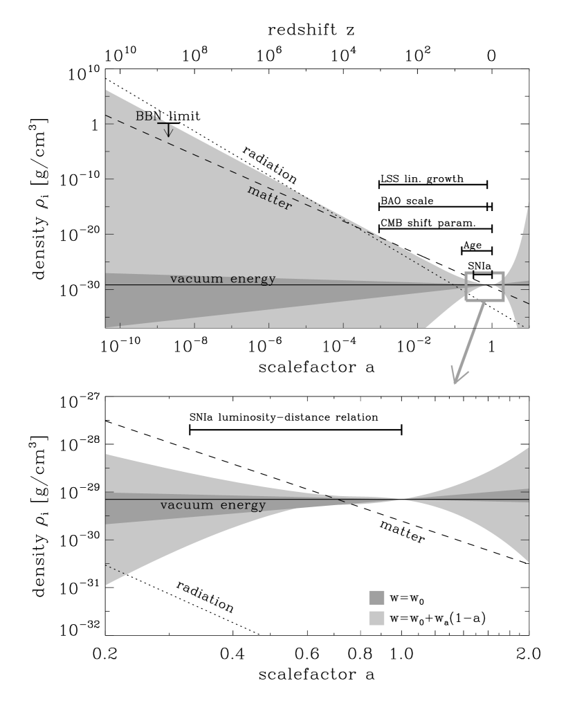
and thus depends on , , and the evolution of the dark energy . The radiation term, irrelevant at low redshifts, can be dropped from Equation 3.3.1. is a dependent parameter due to flatness (). Contemporary datasets include supernovae at redshifts () (Astier et al., 2006; Riess et al., 2007; Wood-Vasey et al., 2007) and provide an effective continuum of constraints on the expansion history over that range (Wang and Tegmark, 2005; Wang and Mukherjee, 2006). The redshift range probed by SNIa is indicated in both panels of Fig. 3.3.
3.3.2 Cosmic Microwave Background
The first peak in the cosmic microwave background (CMB) temperature power spectrum corresponds to density fluctuations on the scale of the sound horizon at the time of recombination. Subsequent peaks correspond to higher-frequency harmonics. The locations of these peaks in -space depend on the comoving scale of the sound horizon at recombination, and the angular distance to recombination. This is summarized by the so-called CMB shift parameter (Efstathiou and Bond, 1999; Elgarøy and Multamäki, 2007) which is related to the cosmology by
| (3.4) |
where (Spergel et al., 2006) is the redshift of recombination. The 3-year WMAP data gives a shift parameter (Davis et al., 2007; Spergel et al., 2006). Since the dependence of Equation 3.4 on and differs from that of Equation 3.2, measurements of the CMB shift parameter can be used to break degeneracies between , and DE evolution in the analysis of SNIa. In the top panel of Fig. 3.3 we represent the CMB observations using a bar from to .
3.3.3 Baryonic Acoustic Oscillations and Large Scale Structure
As they imprinted acoustic peaks in the CMB, the baryonic oscillations at recombination were expected to leave signature wiggles - baryonic acoustic oscillations (BAO) - in the power spectrum of galaxies (Eisenstein and Hu, 1998). These were detected with significant confidence in the SDSS luminous red galaxy power spectrum (Eisenstein et al., 2005). The expected BAO scale depends on the scale of the sound horizon at recombination, and on transverse and radial scales at the mean redshift , of galaxies in the survey. Eisenstein et al. (2005) measured the quantity
| (3.5) |
to have a value , thus constraining the matter density and the dark energy evolution parameters in a configuration which is complomentary to the CMB shift parameter and the SNIa luminosity distance relation. Ongoing BAO projects have been designed specifically to produce stronger constraints on the dark energy equation of state parameter . For example, WIGGLEZ (Glazebrook et al., 2007) will use a sample of high-redshift galaxies to measure the BAO scale at . As well as reducing the effects of non-linear clustering, this redshift is at a larger angular distance, making the observed scale more sensitive to . Constraints from the BAO scale depend on the evolution of the universe from to to set the physical scale of the oscillations. They also depend on the evolution of the universe from to , since the observed angular extent of the oscillations depends on this evolution. The bar representing BAO scale observations in the top panel of Fig. 3.3 indicates both these regimes.
The amplitude of the BAOs - the amplitude of the large scale structure (LSS) power spectrum - is determined by the amplitude of the power spectrum at recombination, and how much those fluctuations have grown (the transfer function) between and . By comparing the recombination power spectrum (from CMB) with the galaxy power spectrum, the LSS linear growth factor can be measured and used to constrain the expansion history of the universe (independently of the BAO scale) over this redshift range. In practice, biases hinder precise normalization of the galaxy power spectrum, weakening this technique. The range over which this technique probes the DE is indicated in Fig. 3.3.
3.3.4 Ages
Cosmological parameters from SN1a, CMB, LSS, BAO and other probes allow us to calculate the current age of the universe to be (Hinshaw, 2006) assuming CDM . Uncertainties on the age calculated in this way grow dramatically if we drop the assumption that the DE is vacuum energy ().
An independent lower limit on the current age of the universe is found by estimating the ages of the oldest known globular clusters (Hansen et al., 2004). These observations rule out models which predict the universe to be younger than ( confidence):
Other objects can also be used to set this age limit Lineweaver (1999), but generally less successfully due to uncertainties in dating techniques.
Assuming CDM , an age of Gyrs corresponds to a redshift of . Contemporary age measurements are sensitive to the dark energy content from to . In the top panel of Fig. 3.3 we show this redshift interval. The evolution and energy content of the universe before Gyrs ago is not probed by these age constraints.
3.3.5 Nucleosynthesis
In addition to the constraints on the expansion history (SN1a, CMB, BAO and ) we know that (at confidence) during Big Bang Nucleosynthesis (BBN) (Bean et al., 2001). Larger dark energy densities imply a higher expansion rate at that epoch () which would result in a lower neutron to proton ratio, conflicting with the measured helium abundance, .
3.3.6 Dark Energy Parameterization
Because of the variety of proposed dark energy models, it has become usual to summarize observations by constraining a parameterized time-varying equation of state. Dark energy models are then confronted with observations in this parameter space. The unique zeroth order parameterization of is (a constant), with characterizing the cosmological constant model. The observational data can be used to constrain the first derivative of . This additional dimension in the DE parameter space may be useful in distinguishing models which have the same . From an observational standpoint, the obvious choice of 1st order parameterization is (di Pietro and Claeskens, 2003). This is rarely used today since currently considered DDE models are poorly portrayed by this functional form. The most popular parameterization is Albrecht et al. (2006); Linder (2006a), which does not diverge at high redshift.
Linder and Huterer (2005) have argued that the extension of this approach to second order, e.g. , is not motivated by current DDE models. Moreover, they have shown that next generation observations are unlikely to be able to distinguish the quadratic from a linear expansion of . Riess et al. (2007) have illustrated this recently using new SN1a.
An alternative technique for exploring the history of dark energy is to constrain or in independent redshift bins. This technique makes fewer assumptions about the specific shape of . In the absence of any strongly motivated parameterization of this bin-wise method serves as a good reminder of how little we actually know from observation. Using luminosity distance measurements from SNIa, DE evolution has been constrained in this way in bins out to redshift (Wang and Tegmark, 2004; Huterer and Cooray, 2005; Riess et al., 2007). In the future, BAO measurements at various redshifts may contribute to these constraints, however will probably never be larger than . Moreover, because the recombination redshift is fixed, only the cumulative effect (from to ) of the DE can be measured with the CMB and LSS linear growth factor. With only this single data point above , the bin-wise technique effectively degenerates to a parameterized analysis at .
3.3.7 Summary of Current DDE Constraints
If one assumes the popular parameterization until last scattering, then all cosmological probes can be combined to constrain and . In a recent analysis of SN1a, CMB and BAO observations, Davis et al. (2007) found and at confidence (the contour is shown in Fig. 3.7). Using the same observations, Wood-Vasey et al. (2007) assumed and found ().
The evolution of is related to by covariant energy conservation (Carroll, 2004)
| (3.7) |
The dark energy density corresponding to the parameterization of is thus given by
| (3.8) |
The cosmic energy density history is illustrated in Fig. 3.3. Radiation and matter densities steadily decline as the dotted and dashed lines. With the DE equation of state parameterized as , its density history is constrained to the light-grey area (Davis et al., 2007). If the evolution of is negligible, i.e. we condition on , then and the DE density history lies within the dark-grey band (Wood-Vasey et al., 2007). If the dark energy is pure vacuum energy (or Einstein’s cosmological constant) then and its density history is given by the horizontal solid black line.
3.4 The Temporal Distribution of Observers
The energy densities , and , and the proximity parameter we imagine we might have observed, depend on the distribution from which we imagine our time of observation has been drawn. What we can expect to observe must be restricted by the conditions necessary for our presence as observers (Carter, 1974). Thus, for example, it is meaningless to suppose we might have lived during inflation, or during radiation domination, or before the first atoms (Dicke, 1961).
We can, however, suppose that we are randomly selected cosmology-discovering observers, and we can expect our observations of and to be typical of observations made by such observers. This is Vilenkin’s principle of mediocrity Vilenkin (1995b). Accordingly, the distribution for the time of observation is proportional to the temporal distribution of cosmology-discovering observers (referred to henceforth as simply “observers”). Thus to solve the coincidence problem one must show that the proximity parameter we measure, , is typical of those measured by other observers.
The most abundant elements in the cosmos are hydrogen, helium, oxygen and carbon (Pagel, 1997). In the past decade extra solar planets have been observed via doppler, transit or microlensing methods. Extrapolation of current patterns in planet mass and orbital period are consistent with the idea that planetary systems like our own are common in the universe (Lineweaver and Grether, 2003). All this does not necessarily imply that observers are common, but it does support the idea that terrestrial-planet-bound carbon-based observers, even if rare, may be the most common observers. In the following estimation of we consider only observers bound to terrestrial planets.
3.4.1 First the Planets…
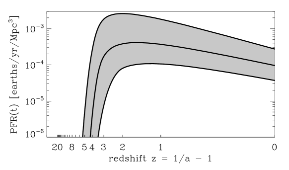
Lineweaver (2001) estimated the terrestrial planet formation rate (PFR) by making a compilation of measurements of the cosmic star formation rate (SFR) and suppressing a fraction of the early stars to correct for the fact that the metallicity was too low for those early stars to host terrestrial planetary systems,
| (3.9) |
In Fig. 3.4 we plot the PFR reported by Lineweaver (2001) as a function of redshift, . As illustrated in the figure, there is large uncertainty in the normalization of the formation history. Our analysis will not depend on the normalization of this function so this uncertainty will not propagate into our analysis. There are also uncertainties in the location of the turnover at high redshift, and in the slope of the formation history at low redshift - both of these will affect our results.
The conversion from redshift to time depends on the particular cosmology, through the Friedmann equation,
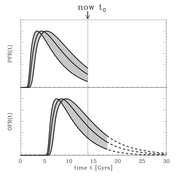
In Fig. 3.5 we plot the PFR from Fig. 3.4 as a function of time assuming the best fit parameterized DDE cosmology.
3.4.2 … then First Observers
After a star has formed, some non-trivial amount of time will pass before observers, if they arise at all, arise on an orbiting rocky planet. This time allows planets to form and cool and, possibly, biogenesis and the emergence observers. is constrained to be shorter than the life of the host star. If we consider that our has been drawn from a probability distribution . The observer formation rate (OFR) would then be given by the convolution
| (3.11) |
In practice we know very little about . It must be very nearly zero below about - this is the amount of time it takes for terrestrial planets to cool and the bombardment rate to slow down. Also, it must be near zero above the lifetime of a small () star (above ). If we assume that our is typical, then has significant weight around - the amount of time it has taken for us to evolve here on Earth.
A fiducial choice, where all observers emerge after the formation of their host planet, is . This choice results in an OFR whose shape is the same as the PFR, but is shifted into the future,
| (3.12) |
(see the lower panel of Fig. 3.5). Even for non-standard and values, this fiducial OFR aligns closely with the peak and the effect of a wider is generally to increase the severity of the coincidence problem by spreading observers outside the peak. Hence using our fiducial (which is the narrowest possibility) will lead to conclusions which are conservative in that they underestimate the severity of the cosmic coincidence. If another choice for could be justified, the cosmic coincidence would be more severe than estimated here. We will discuss this choice in Section 3.6.
The OFR is then extrapolated into the future using a decaying exponential with respect to (the dashed segment in the lower panel of Fig. 3.5). The observed SFH is consistent with a decaying exponential. We have tested other choices (linear & polynomial decay) and our results do not depend strongly on the shape of the extrapolating function used.
The temporal distribution of observers is proportional to the observer formation rate,
| (3.13) |
This observer distribution is similar to the one used by Garriga et al. (1999) to treat the coincidence problem in a multiverse scenario. By comparison, our distribution starts later because we have considered the time required for the build up of metallicity, and because we have included an evolution stage of . Our distribution also decays more quickly than theirs does. Some of our cosmologies suffer big-rip singularities in the future. In these cases we truncate at the big-rip.
3.5 Analysis and Results: Does fitting contemporary constraints necessarily solve the cosmic coincidence?
For a given model the proximity parameter observed by a typical observer is described by a probability distribution calculated as
| (3.14) |
The summation is over contributions from all solutions of (typically, any given value of occurs at multiple times during the lifetime of the Universe). In Fig. 3.6 we plot for the , cosmology. In this case, observers are distributed over a wide range of values, with seeing , and seeing .

We define the severity of the cosmic coincidence problem as the probability that a randomly selected observer measures a proximity parameter lower than we do:
| (3.15) |
For the , cosmology of Figs. 3.5 and 3.6, the severity is . This model does not suffer a coincidence problem since of observers would see lower than we do. If the severity of the cosmic coincidence would be near () in a particular model, then that model would suffer a () coincidence problem and the value of we observe really would be unexpectedly high.
We calculated the severities for cosmologies spanning a large region of the plane and show our results in Fig. 3.7 using contours of equal . The severity of the coincidence problem is low (e.g. ) for most combinations of and shown. There is a coincidence problem, where the severity is high (), in two regions of this parameter space. These are indicated in Fig. 3.7.
Some features in Fig. 3.7 are worth noting:
-
•
Dominating the left of the plot, the severity of the coincidence increases towards the bottom left-hand corner. This is because as and become more negative, the peak becomes narrower, and is observed by fewer observers.
-
•
There is a strong vertical dipole of coincidence severity centered at . For there is a large coincidence problem because in such models we would be currently witnessing the very closest approach between DE and matter, with for all earlier and later times (see Fig. 3.8c). For there is an anti-coincidence problem because in those models we would be currently witnessing the DDE’s furthest excursion from the matter density, with and in closer proximity for all relevant earlier and later times, i.e., all times when is non-negligible.
-
•
There is a discontinuity in the contours running along for phantom models (). The distribution is truncated by big-rip singularities in strongly phantom models (provided they remain phantom; ). This truncation of late-time observers means that early observers who witness large values of represent a greater fraction of the total population.
To illustrate these features, Fig. 3.8 shows the density histories and observer distributions for four specific examples selected from the plane of Fig. 3.7.
We find that all observationally allowed combinations of and result in low severities (), i.e., there are large () probabilities of observing the matter and vacuum density to be at least as close to each other as we observe them to be.
3.6 Discussion
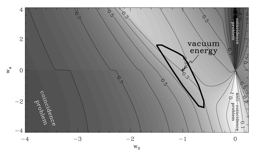
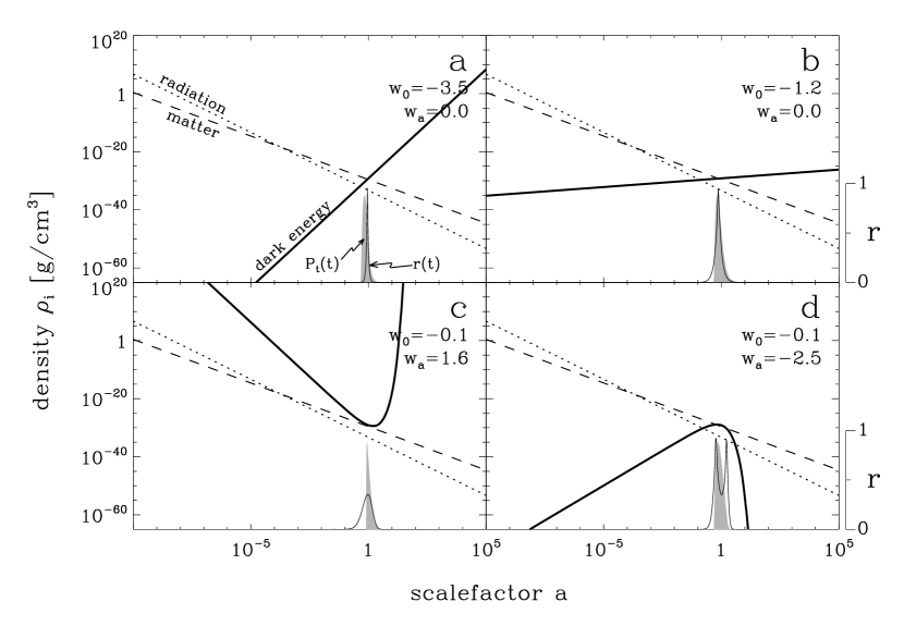
It was not clear what DDE dynamics were required to solve the coincidence problem. Our analysis might have resulted in new constraints on the values of and , by simply demanding that we do not live during a special time in which . There are regions of parameter space that can be ruled out in this manner (see Fig. 3.7) however those points are already strongly excluded by observational constraints on and . Therefore, the cosmic coincidence problem can not be used as a tool to further constrain DDE since the problem is solved for all DDE models satisfying observational constraints on and .
The main result of our analysis is that any DDE model in agreement with current cosmological constraints has for a significant fraction of observers.
Interacting quintessence models in which the proximity parameter asymptotes to a constant at late times (Amendola, 2000a; Zimdahl et al., 2001; Amendola and Quercellini, 2003; França and Rosenfeld, 2004; Guo and Zhang, 2005; Olivares et al., 2005; Pavón and Zimdahl, 2005; Zhang, 2005; França, 2006; Amendola et al., 2006, 2007; Olivares et al., 2007) have been proposed as a solution to the coincidence problem. More recently, del Campo et al. (2005, 2006) have argued for a broader class of interacting quintessence models that “soften” the coincidence problem by predicting a very slowly varying (though not constant) proximity parameter. Our analysis finds that need not asymptote to a constant, nor evolve particularly slowly, partially undermining the motivations for these interacting quintessence models.
Caldwell et al. (2003) and Scherrer (2005) have proposed that the coincidence problem may be solved by phantom models in which there is a future big-rip singularity because such cosmologies spend a significant fraction of their lifetimes in states. In our work is terminated by big-rip singularities in ripping models. In non-ripping models, however, the distribution is effectively terminated by the declining star formation rate. Therefore the big-rip gives phantom models only a marginal advantage over other models. This marginal advantage manifests as the discontinuity along on the left side of Fig. 3.7.
We could improve our analysis, in the sense of getting tighter coincidence constraints (larger severities), if we used a less conservative . We used the most conservative choice - a delta function - because the present understanding of the time it takes to evolve into observers is too poorly developed to motivate any other form of . Another possible improvement is the DE equation of state parameterization. We used the current standard, , which may not parameterize some models well for very small or very large values of .
We conclude that DDE models need not be fitted with exact tracking or oscillatory behaviors specifically to solve the coincidence by generating long or repeated periods of . Also, particular interactions guaranteeing for long periods are not well motivated. Moreover phantom models have no significant advantage over other DDE models with respect to the coincidence problem discussed here.
ACKNOWLEDGMENTS
CE acknowledges a UNSW School of Physics postgraduate fellowship. CE thanks the ANU’s RSAA for its kind hospitality, where this research was carried out.
Appendix A: Numerical Values for Parameters of Models Illustrated in Fig. 3.2
| Model | Parameter | Value |
|---|---|---|
| power law tracker quintessence | ||
| exponential tracker quintessence | ||
| tracking oscillating energy | ||
| interacting quintessence | ||
| Chaplygin gas | ||
Chapter 4 Comparing the Sun to Other Stars: Searching for Life Tracers Amongst the Solar Properties
Here comes the Sun,
here comes the Sun,
and I say it’s alright.
- The Beatles, “Here Comes the Sun”
4.1 Introduction
In the past decade the first several hundred extra-solar planets have been detected using various techniques. These techniques are all biased towards massive planets in small orbits (so-called hot Jupiters). The next generation of projects (including NASA’s Terrestrial Planet Finder and ESA’s Darwin Project) is eagerly anticipated, with the discovery of Earth-like planets orbiting within habitable zones expected. In the mean time, the search for solar twins (stars with properties most like those of the Sun) in stellar surveys, continues. The reason behind our fascination with Earth-like planets and Sun-like stars is that without a thorough understanding of the requirements of life, a reasonable strategy in the search for extra terrestrial life is to look in environments that we know are capable of hosting life, i.e. those planets and stars which are most like our own.
If the emergence of life and observers on a planet depends on special properties of the planet’s host star, then we would expect our Sun to exhibit those properties and stand out when compared to a sample of randomly selected stars. In this way, the comparison of the Sun to other stars may be a way of identifying stellar properties important to the origin of life and the evolution of observers.
What we stand to gain by looking for anomalous properties in the Sun are statements about the dependence of life on various stellar properties (the reliability of which can be quantified). Such information could be used to improve searches for life in the universe by focussing them on the most important properties.
An early example of this type of work is Gonzalez (1999a, b) who proposed, based on his findings that the Sun was more massive than of all stars, that life may exist preferentially around high-mass stars.
Taken together however, previous work of this type is inconsistent in its conclusions. While Gonzalez (1999a, b); Gonzalez et al. (2001) suggested the Sun to be anomalous, Gustafsson (1998); Allende Prieto (2006) found it to be typical. These discrepancies result from inconsistent use of language, stellar sample selection and inconsistency in the choice of stellar/solar properties compared.
In order to clarify these issues we have undertaken a joint -parameter analysis that compares the Sun to representative samples of stars in independent properties plausibly related to life and habitability. The analysis quantifies the degree of (a)typicality of the Sun and draws conclusions about the legitimacy of postulated links between particular properties and habitability.
4.2 Selection of Solar Properties and Stellar Samples
Since the purpose of our analysis is to identify significantly anomalous solar properties (or a lack thereof), it is important that our selection criteria is not dependent on any prior knowledge we may have about the (a)typicality of the Sun with respect to its properties. Intentionally selecting one (or a few) parameters in which the Sun is known to be anomalous would pre-load the result.
Suppose, for example, that the Sun has previously been compared to representative samples of stars in uncorrelated parameters, none of which play any significant role in determining habitability. It should be expected that the Sun is a (-percentile) outlier in one in these parameters (call it ) just by pure chance. If the present analysis were conducted using just , naive that had been selected, the results would erroneously suggest that was related to habitability.
On the other hand, the indiscriminant inclusion of properties unlikely to have any connection to habitability could dilute a legitimate signal. Suppose that is a stellar property, and that only stars in the upper with respect to are capable of hosting life (the upper are amongst the -percentile outliers). The signal can be diluted away by including other parameters (and can be reduced to a signal by including just other parameters).
No single stellar survey contains unbiased measurements in as many parameters as we are interested in, and for this reason we have used different stellar samples for each parameter. The benefit of being able to choose the best available sample for each parameter comes at a cost, which is that we must eliminate any correlated parameters from our analysis.
With the above considerations in mind, we have included maximally uncorrelated stellar properties all of which are plausibly related to habitability and for which a sufficiently large unbiased sample of stellar values exists. The included properties come from a full set of candidates (refer to Robles et al. (2008b) for the full list and correlation analysis). Below we give a brief description of the included properties, along with a brief description of their relevance to habitability and a description of the stellar samples we have used for each.
-
1.
Mass: The mass of a star is arguably the most important property of a star. It determines luminosity, temperature and main sequence longevity, in turn influencing conditions and stability in the circumstellar habitable zone. Low mass stars are intrinsically dim, so large stellar samples are biased towards high-mass stars. We have used the nearest stars from the RECONS compilation (Henry, 2006), which is complete to .
-
2.
Age: If the evolution of observers takes (on average) much longer than typical lifetime of a star (Carter, 1983) then observers may be expected to arise preferentially around older stars. We construct an age distribution for stars in the galaxy using galactic star formation history from Rocha-Pinto et al. (2000). Their star formation history is based on chromospheric ages of dwarf stars at up to , and has been corrected for scale-height, stellar evolution and volume incompleteness. We also consider the cosmic age distribution, using the cosmic star formation history from Hopkins (2006).
-
3.
Metallicity [Fe/H]: A star’s iron content is a good proxy for its abundance in other elements heavier than helium. With regard to this analysis, metallically is correlated with abundance of the ingredients for terrestrial planets (O, Fe, Si and Mg) and life (C, O, N and S). We use the sample of FGK stars of Grether and Lineweaver (2006, 2007) selected from the Hipparcos catalogue. This sample is complete to for stars within the spectral range - and absolute magnitude of (Reid, 2002) and contains metallicities derived from a range of spectroscopic and photometric surveys.
-
4.
Carbon-to-oxygen ratio [C/O]: The relative abundance of carbon to oxygen impacts the abundance of oxygen (and the balance of REDOX chemistry) in the circumstellar habitable zone. If [C/O] is higher than , most oxygen forms carbon monoxide which is subsequently cleared by stellar winds leaving a chemically reducing habitable zone (Kuchner and Seager, 2005). For our stellar distribution in [C/O] we use stars from Gustafsson et al. (1999); Reddy et al. (2003); Bensby and Feltzing (2006).
- 5.
-
6.
Rotational velocity : The rotational velocity of a star is related to the angular momentum of the protoplanetary disk. A low rotational velocity may be correlated with the presence of planets (Soderblom, 1983). We use the subset of stars in the - mass range from the sample of Valenti and Fischer (2005). By cutting near the solar value in mass we minimize the effects of a known correlation between stellar mass and which becomes significant at higher masses.
-
7.
Eccentricity of the star’s galactic orbit : The galactic orbit of a star determines the stellar environments that the star passes through. Stars with highly eccentric orbits pass closer to the galactic center where the risk of a nearby supernova, and the flux of potentially harmful radiation is higher. We use the distribution of stellar eccentricities from stars witin as computed by Nordström et al. (2004).
-
8.
Maximum height away from the galactic plane : As the Sun oscillates through the thin disk of the galaxy objects in the Oort cloud may be disrupted by tidal gravitational forces. It is plausible that the frequency of such disruptions (for which is a proxy) influences the frequency of impacts on planets in the habitable zone. For we use the same stellar sample as we did for eccentricity.
-
9.
Mean galactocentric radius : The mean galactocentric radius is the most important of a star’s galactic orbital properties. It determines (to a greater degree than eccentricity for typical eccentricities) the minimum approach to the galactic center, the risk of nearby supernova, and the flux of potentially harmful radiation from the galactic center. Our distribution of is based on the model of Bahcall and Soneira (1980) assuming a scale length of (Gould et al., 1996).
-
10.
The stellar mass of the star’s host galaxy : This influences the overall (galactic) metallically, including the metallically of the star’s neighbourhood. We construct a distribution of based on the -band luminosity function of Loveday (2000) and assume a constant stellar-mass-to-light ratio of (Bell and de Jong, 2001). It is important to note that we are interested in the distribution of stars in , not the distribution of galaxies in .
-
11.
The stellar mass of the star’s host group of galaxies : This is correlated with the density of the galactic environment. This influences the stability of the host galaxy. We use the -band luminosity distribution of galactic groups from the 2dFGRS Percolation-Inferred Galaxy Groups catalogue (Eke et al., 2004) and assume a constant stellar-mass-to-light ratio of 1.5 (Bell and de Jong, 2001). As for host galaxy mass, we are interested in the distribution of stars in , not the distribution of groups in .
4.3 Analysis and Results
The solar values of the selected properties are taken (or derived from related properties) from the literature. The solar values are shown in Table 4.1.
| Parameter | Solar Value | Median Value | ||
|---|---|---|---|---|
| Mass | ||||
| Age | ||||
a. By definition.
b. Chromospheric age of the Sun from Wright et al. (2004).
c. Rotational velocity at the surface is (Valenti and Fischer, 2005). We calculate a which may be compared to our stellar distribution by apply a factor of (the average over of over a -sphere; this simulates randomizing the inclination at which the Sun is viewed).
d. The eccentricity of the Sun’s galactic orbit is calculated from solar motion reported in Dehnen and Binney (1998).
e. Found by integrating the solar orbit in the galactic potential (initial motion as reported in Dehnen and Binney (1998)).
f. Eisenhauer et al. (2005)
g. Derived in the same way as our distribution: by applying a stellar-mass-to-light ratio to the -band luminosity. The -band luminosity is inferred from the -band measured by Courteau and van den Bergh (1999) using the mean color of an Sbc spiral galaxy from the 2MASS Large Galaxy Atlas (Jarrett et al., 2003) and the color conversion prescription of Driver et al. (1994).
h. Derived in the same way as our distribution: by applying a stellar-mass-to-light ratio to the -band luminosity of 2PIGG and Local Group galaxies from Courteau and van den Bergh (1999).
. These distributions span several orders of magnitude and are analyzed in -space. The values for and represent widths measured in -space.
We find the median and the and percentiles for each of the distributions. of a distribution is between the and percentiles, and in the case of a Gaussian distribution this interval corresponds to the interval.
Our distributions are generally asymmetric. Since we are calculating the deviation of the Sun from the mean stellar sample we are most interested in the width of the distributions in the direction of the solar value. We define as the difference between the median and the or percentile, depending on whether the solar value is below or above the median.
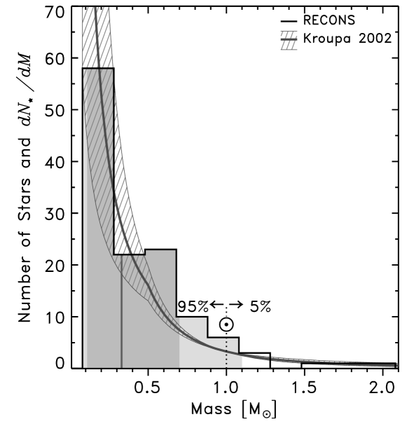
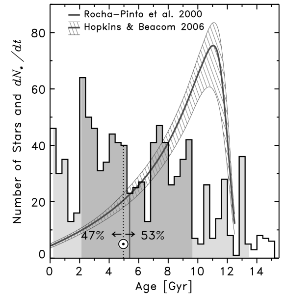
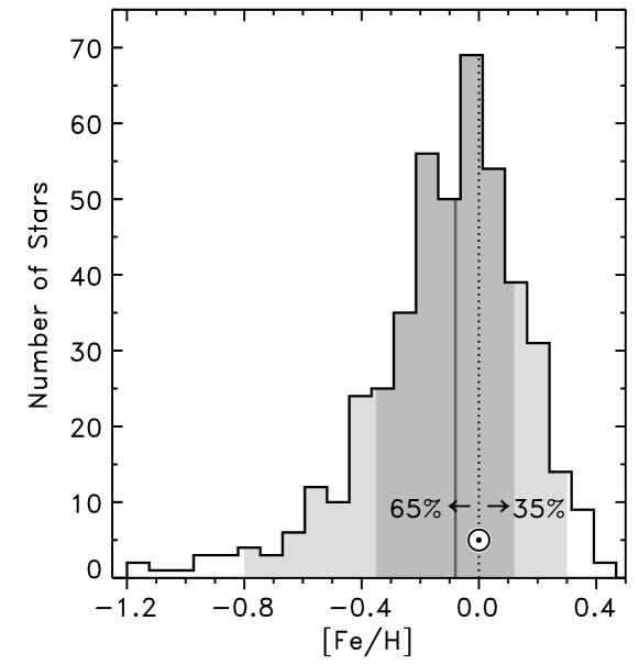
The medians and widths of the stellar distributions are shown in the last two columns of Table 4.1. Figures 4.1, 4.2 and 4.3 show the stellar distributions in first three properties: mass, age and metallicity. These figures have been included as examples. The equivalent figures for parameters - are omitted from this summary, but can be found in the reviewed publication of this work (Robles et al., 2008b).
We compute the combined deviation of the solar properties from those of an average star using the statistic.
| (4.1) |
While uncertainties in the solar values are propagated directly, we employ a bootstrap (Efron, 1979) to account for the uncertainties in and due to small number statistics. This involves randomly repeatedly resampling the distributions (from the original samples, but allowing the same star to be drawn multiple times), and calculating the corresponding , and each time.
We find the combined -parameter solar chi-square to be
| (4.2) |
The probability of selecting, at random, a star which is more normal than the Sun (a star with a lower ) can be calculated using the standard distribution for degrees of freedom.
| (4.3) |
The probability calculated above relies on the assumption that our properties are normally distributed. Since several of our distributions are poorly approximated by Gaussians (for example age, see Figure 4.2), we have performed a Monte Carlo simulation (Metropolis and Ulam, 1949) to calculate a more accurate value of . In the Monte Carlo simulation a large number of stars are randomly selected from our distributions and their are calculated (according to equation 4.1). In this way we find that the probability of randomly selecting a star more normal than the Sun is
| (4.4) |
4.4 Discussion
Of the stellar properties included in this study, the Sun is most anomalous in its mass (more massive than stars in our sample), in the eccentricity of its galactic orbit (which is lower than of stars in our sample) and in its rotational velocity (which is slower than of stars in our sample). Panel A of figure 4.4 illustrates how the solar values compare to the and intervals for each of the parameters. The levels of solar anomaly for each of the properties are shown in Panel D as a percentile, and in terms of the number of standard deviations from the median.
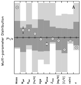 |
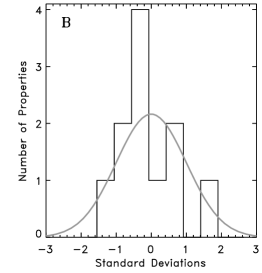 |
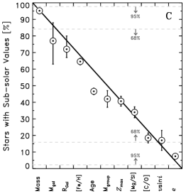 |
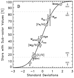 |
A. Comparing the solar values to the (dark grey) and (light grey) intervals for each parameter. The horizontal line represents the median of each of the distributions, and the vertical axis is normalized to the longer of the two intervals for each of the distributions.
B. A histogram of the distribution of parameters in standard deviation compared to a gaussian.
C. The percentage of stars with sub-solar values for each of the parameters in decreasing order of . The line represents the expected arrangement of points “” for randomized parameter values. Significant deviations from the line may indicate unexpected anomalies, none of which are seen here.
D. Each of the solar properties is plotted in -standard deviation space. If the distributions were Gaussian the points would fall along the solid line.
When mass, eccentricity and rotational velocity are combined with our other parameters, which are also plausibly related to habitability, the Sun looks entirely mediocre. The probability of selecting a star, at random, which is more typical than the Sun with respect to these parameters is only .
This result undermines suggestions that an anthropic explanation is required for the Sun’s unusually large mass. The alternative explanation, which is defended by our results is that in measuring the properties of the Sun we have come across a few mild outliers - as few and as mild as we should expect for a random star, given the number of properties measured. A convenient visualization of this is given in Panel C of figure 4.4. The properties are arranged in decreasing order of , where is the percentage of stars with sub-solar values in a given property. When arranged in this way, we expect the parameters to be near the line given by
| (4.5) |
where is the number of parameters. Any anomalies that cannot be attributed to noise would appear up as points significantly far from the line.
We have repeated the analysis without mass and eccentricity and find the Sun to be unexpectedly average: only of stars are more average than the Sun with respect to the remaining parameters. This supports the proposition that the anomalies observed in mass and eccentricity are expected by pure chance. By including just mass and eccentricity, we find that the Sun is more anomalous than of stars. This would be some evidence () for an anthropic explanation for one or both of these properties, if they had not been selected to ensure this result.
Our parameter selection criteria selected a larger number of properties plausibly related to life. Without strong evidence suggesting that any are more important than any other, they have been treated equally. A potential extension of this work would be the inclusion of factors to weight the plausibility (based on planetary formation models and biology) that a property is related to life.
Chapter 5 A Larger Estimate of the Entropy of the Universe
We are all
made of stars.
We were created in the birth of stars.
- Encounter, “Starborn”
5.1 Introduction
The entropy budget of the universe is important because its increase is associated with all irreversible processes, on all scales, across all facets of nature: gravitational clustering, accretion disks, supernovae, stellar fusion, terrestrial weather, and chemical, geological and biological processes (Frautschi, 1982; Lineweaver and Egan, 2008).
Recently, Frampton et al. (2008) and Frampton and Kephart (2008) reported the entropy budget of the observable universe. Their budgets (listed aside others in Table 5.1) estimate the total entropy of the observable universe to be , dominated by the entropy of supermassive black holes (SMBHs) at the centers of galaxies. That the increase of entropy has not yet been capped by some limiting value, such as the holographic bound (’t Hooft, 1993; Susskind, 1995) at (Frampton et al., 2008), is the reason dissipative processes are ongoing and that life can exist.
In this paper, we improve the entropy budget by using recent observational data and quantifying uncertainties. The paper is organized as follows. In what remains of the Introduction, we describe two different schemes for quantifying the increasing entropy of the universe, and we comment on caveats involving the identification of gravitational entropy. Our main work is presented in Sections 5.2 and 5.3, where we calculate new entropy budgets within each of the two accounting schemes. We finish in Section 5.4 with a discussion touching on the time evolution of the budgets we have calculated, and ideas for future work.
Throughout this paper we assume flatness () as predicted by inflation (Guth, 1981; Linde, 1982) and supported by observations (Spergel et al., 2007). Adopted values for other cosmological parameters are , , (Seljak et al., 2006), and (Mather et al. 1999; quoted uncertainties are ).
5.1.1 Two Schemes for Quantifying the Increasing Entropy of the Universe
Modulo statistical fluctuations, the generalized second law of thermodynamics holds that the entropy of the universe (including Bekenstein-Hawking entropy in the case of any region hidden behind an event horizon), must not decrease with time (Bekenstein, 1974; Gibbons and Hawking, 1977). Within the FRW framework, the generalized second law can be applied in at least two obvious ways:
-
1.
The total entropy in a sufficiently large comoving volume of the universe does not decrease with cosmic time,
(5.1) -
2.
The total entropy of matter contained within the cosmic event horizon (CEH) plus the entropy of the CEH itself, does not decrease with cosmic time,
(5.2)
In the first of these schemes, the system is bounded by a closed comoving surface. The system is effectively isolated because large-scale homogeneity and isotropy imply no net flows of entropy into or out of the comoving volume. The time-slicing in this scheme is along surfaces of constant cosmic time. Event horizons of black holes are used to quantify the entropy of black holes, however the CEH is neglected since the assumption of large-scale homogeneity makes it possible for us to keep track of the entropy of matter beyond it. A reasonable choice for the comoving volume in this scheme is the comoving sphere that presently corresponds to the observable universe, i.e., the gray area in Figure 5.1. Correspondingly, in Section 5.2 we calculate the present entropy budget of the observable universe and we do not include the CEH.
The second scheme is similar to the first in that we time-slice along surfaces of constant cosmic time. However, here the system (yellow shade in Figure 5.1) is bounded by the time-dependent CEH instead of a comoving boundary. Migration of matter across the CEH is not negligible, and the CEH entropy (Gibbons and Hawking, 1977) must be included in the budget to account for this (e.g. Davis et al. 2003). The present entropy of the CEH and its interior is calculated in Section 5.3.
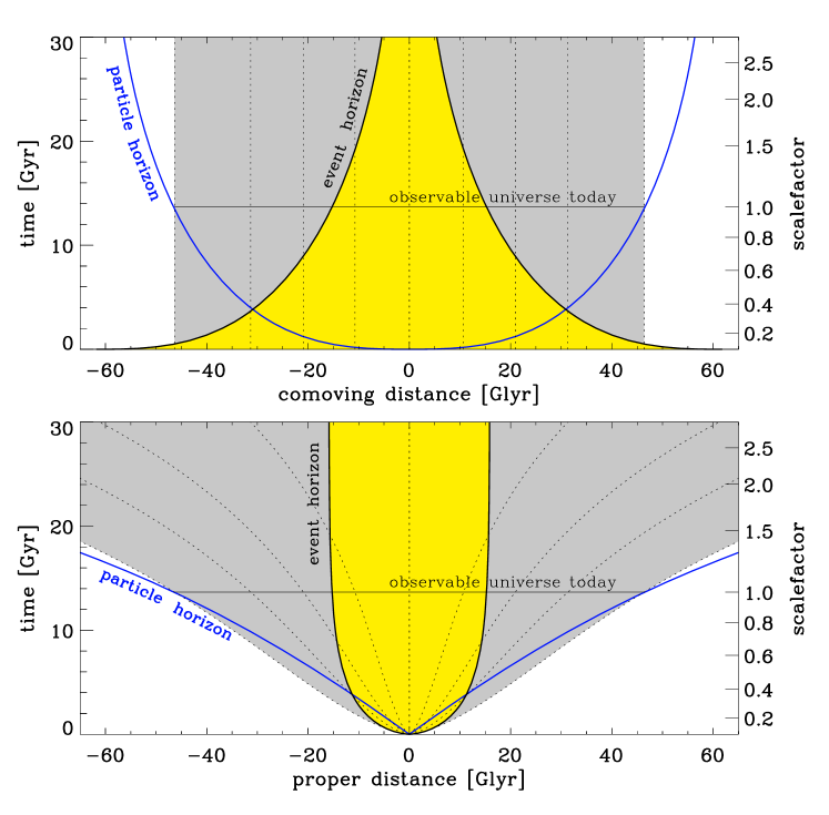
5.1.2 Entropy and Gravity
It is widely appreciated that non-gravitating systems of particles evolve toward homogenous temperature and density distributions. The corresponding increase in the volume of momentum-space and position-space occupied by the constituent particles represents an increase in entropy. On the other hand, strongly gravitating systems become increasingly lumpy. With “lumpyness” naively akin to “orderliness”, it is not as easy to see that the total entropy increases. In these systems the entropy is shared among numerous components, all of which must be considered.
For example, approximately collisionless long-range gravitational interactions between stars result in dynamical relaxation of galaxies (whereby bulk motions are dissipated and entropy is transferred to stars in the outer regions of the galaxy; Lynden-Bell 1967) and stellar evaporation from galaxies (whereby stars are ejected altogether, carrying with them energy, angular momentum and entropy, and allowing what remains behind to contract; e.g. Binney and Tremaine 2008). In more highly dissipative systems, i.e., accretion disks, non-gravitational interactions (viscosity and/or magnetorotational instability; Balbus and Hawley 2002) transfer angular momentum and dissipate energy and entropy.
In addition to these considerations, entropy also increases when gravitons are produced. A good example is the in-spiral of close binaries, such as the Hulse-Taylor binary pulsar system (Hulse and Taylor, 1975; Weisberg and Taylor, 2005). Gravitational waves emitted from the system extract orbital energy (and therefore entropy) allowing the system to contract.
The entropy of a general gravitational field is still not known. Penrose (1987, 1979, 2004) has proposed that it is related to the Weyl curvature tensor . In conformally flat spacetimes (such as an ideal FRW universe), the Weyl curvature vanishes and gravitational entropy is postulated to vanish (to limits imposed by quantum uncertainty). In clumpy spacetimes the Weyl curvature takes large values and the gravitational entropy is high. While Ricci curvature vanishes in the absence of matter, Weyl curvature may still be non-zero (e.g. gravitational waves traveling though empty space) and the corresponding gravitational entropy may be non-zero.
If these ideas are correct then the low gravitational entropy of the early universe comes from small primordial gravitational perturbations. Gravitational entropy then increases with the growing amplitude of linear density fluctuations parameterized through the matter power spectrum . The present gravitational entropy, however, is expected to be dominated by the nonlinear overdensities (with large Weyl tensors) which have formed since matter-radiation equality.
In extreme cases, gravitational clumping leads to the formation of black holes. The entropy of black holes is well known (Bekenstein, 1973; Hawking, 1976; Strominger and Vafa, 1996). The entropy of a Schwarzschild black hole is given by
| (5.3) |
where is the event-horizon area and is the black hole mass.
Because gravitational entropy is difficult to quantify, we only include it in the two extremes: the thermal distribution of gravitons and black holes.
5.2 The Present Entropy of the Observable Universe
The present entropy budget of the observable universe was estimated most recently by Frampton et al. (2008) and Frampton and Kephart (2008). Those papers and earlier work (Kolb and Turner, 1981; Frautschi, 1982; Penrose, 2004; Bousso et al., 2007) identified the largest contributors to the entropy of the observable universe as black holes, followed distantly by the cosmic microwave background (CMB) and the neutrino background. The last column of Table 5.1 contains previous estimates of the entropy in black holes, the CMB and neutrinos, as well as several less significant components.
Sections 5.2.1 – 5.2.7 below describe the data and assumptions used to calculate our entropy densities (given in Column 2 of Table 5.1). Our entropy budget for the observable universe (Column 3 of Table 5.1) is then found by multiplying the entropy density by the volume of the observable universe ,
| (5.4) |
where is the entropy density of component . The volume of the observable universe is (see Appendix)
| (5.5) | |||||
| Component | Entropy Density | Entropy | Entropy (previous work) |
|---|---|---|---|
| SMBHs | , , | ||
| Stellar BHs | , | ||
| Photons | , | ||
| Relic Neutrinos | , | ||
| WIMP Dark Matter | |||
| Relic Gravitons | |||
| ISM and IGM | |||
| Stars | |||
| Total | , , | ||
| Tentative Components: | |||
| Massive Halo BHs | |||
| Stellar BHs |
5.2.1 Baryons
For a non-relativistic, non-degenerate gas the specific entropy (entropy per baryon) is given by the Sakur-Tetrode equation (e.g. Basu and Lynden-Bell 1990)
| (5.6) |
where indexes particle types in the gas, is the th particle type’s number density, and is its internal partition function. Basu and Lynden-Bell (1990) found specific entropies between and per baryon for main-sequence stars of approximately solar mass. For components of the interstellar medium (ISM) and intergalactic medium (IGM) they found specific entropies between ( in the ISM) and (ionized hydrogen in the IGM) per baryon.
The cosmic entropy density in stars can be estimated by multiplying the specific entropy of stellar material by the cosmic number density of baryons in stars :
| (5.7) |
Using the stellar cosmic density parameter (Fukugita and Peebles, 2004), and the range of specific entropies for main-sequence stars around the solar mass (which dominate stellar mass), we find
| (5.8) | |||||
| (5.9) |
Similarly, the combined energy density for the ISM and IGM is (Fukugita and Peebles, 2004), and by using the range of specific entropies for ISM and IGM components, we find
| (5.10) | |||||
| (5.11) |
The uncertainties in Equations (5.9) and (5.11) are dominated by uncertainties in the mass weighting of the specific entropies, but also include uncertainties in , and the volume of the observable universe.
5.2.2 Photons
The CMB photons are the most significant non-black hole contributors to the entropy of the observable universe. The distribution of CMB photons is thermal (Mather et al., 1994) with a present temperature of (Mather et al., 1999).
5.2.3 Relic Neutrinos
The neutrino entropy cannot be calculated directly since the temperature of cosmic neutrinos has not been measured. Standard treaties of the radiation era (e.g. Kolb and Turner 1990; Peacock 1999) describe how the present temperature (and entropy) of massless relic neutrinos can be calculated from the well known CMB photon temperature. Since this background physics is required for Sections 5.2.4 and 5.2.5, we summarize it briefly here.
A simplifying feature of the radiation era (at least at known energies ) is that the radiation fluid evolves adiabatically: the entropy density decreases as the cube of the increasing scalefactor . The evolution is adiabatic because reaction rates in the fluid are faster than the expansion rate of the universe. It is convenient to write the entropy density as
| (5.14) |
where is the number of relativistic degrees of freedom in the fluid (with ) given approximately by
| (5.17) |
For photons alone, , and thus Equation (5.14) becomes Equation (5.2.2). For photons coupled to an electron-positron component, such as existed before electron-positron annihilation, .
As the universe expands, massive particles annihilate, heating the remaining fluid. The effect on the photon temperature is quantified by inverting Equation (5.14),
| (5.18) |
The photon temperature decreases less quickly than because decreases with time. Before electron-positron annihilation the temperature of the photons was the same as that of the almost completely decoupled neutrinos. After annihilation, heats only the photons, the two temperatures differ by a factor ,
| (5.19) |
A reasonable approximation is derived by assuming that only photons were heated during annihilation, where is the ratio of for photons to for photons, electrons, and positrons.
Corrections are necessary at the level because neutrinos had not completely decoupled at annihilation (Gnedin and Gnedin, 1998). The neutrino entropy density is computed assuming a thermal distribution with , and we assign a uncertainty.
| (5.20) | |||||
where ( flavors, spin states each). The total neutrino entropy in the observable universe is then
| (5.21) |
with an uncertainty dominated by uncertainty in the volume of the observable universe.
Neutrino oscillation experiments have demonstrated that neutrinos are massive by measuring differences between the three neutrino mass eigenstates (Cleveland et al., 1998; Adamson et al., 2008; Abe et al., 2008). At least two of the mass eigenstates are heavier than . Since this is heavier than their current relativistic energy (; computed under the assumption that they are massless) at least two of the three masses are presently non-relativistic.
Expansion causes non-relativistic species to cool as instead of , which would result in a lower temperature for the neutrino background than suggested by Equation (5.19). The entropy density (calculated in Equation 5.20) and entropy (calculated in Equation 5.21) are unaffected by the transition to non-relativistic cooling since the cosmic expansion of relativistic and non-relativistic gases are both adiabatic processes (the comoving entropy is conserved, so in either case ).
We neglect a possible increase in neutrino entropy due to their infall into gravitational potentials during structure formation. If large, this will need to be considered in future work.
5.2.4 Relic Gravitons
A thermal background of gravitons is expected to exist, which decoupled from the photon bath around the Planck time, and has been cooling as since then. The photons cooled less quickly because they were heated by the annihilation of heavy particle species (Equation 5.18). Thus we can relate the current graviton temperature to the current photon temperature
| (5.22) |
where is the number of relativistic degrees of freedom at the Planck time and today (this is appropriate even in the case of massive neutrinos because they decoupled from the photon bath while they were still relativistic). Given the temperature of background gravitons, their entropy can be calculated as
| (5.23) |
where .
Figure 5.2 shows as a function of temperature. The function is well known for temperatures below about , but is not known at higher temperatures. Previous estimates of the background graviton entropy have assumed (Frampton et al., 2008; Frampton and Kephart, 2008), but this should be taken as a lower bound on yielding an upper bound on and .
To get a better idea of the range of possible graviton temperatures and entropies, we have adopted three values for . As a minimum likely value we use (Figure 5.2, thick blue line), which includes the minimal set of additional particles suggested by supersymmetry. As our middle value we use , corresponding to the linear extrapolation of in to the Planck scale (Figure 5.2, gray line). And as a maximum likely value we use , corresponding to an exponential extrapolation (Figure 5.2, thin blue line).
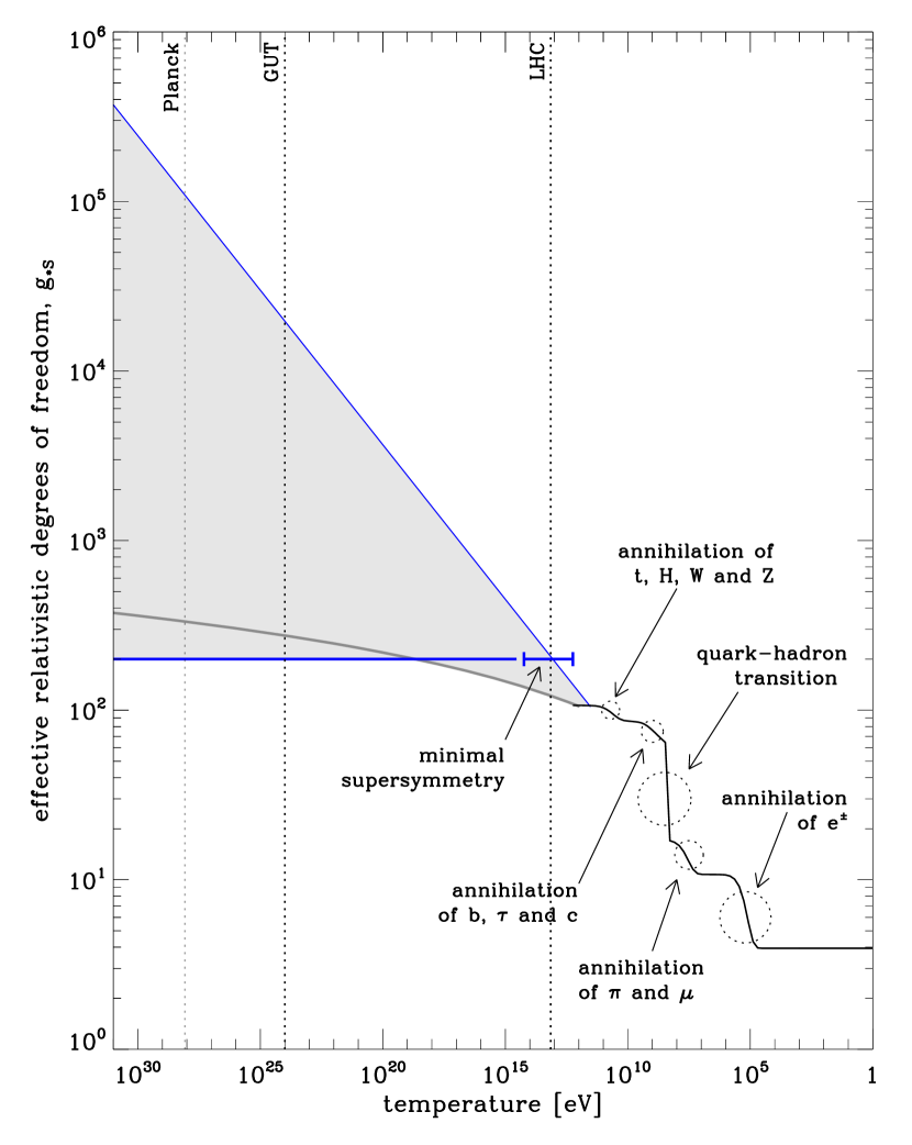
The corresponding graviton temperatures today are (Equation 5.22)
| (5.24) |
Inserting this into Equation (5.23) we find the entropy in the relic graviton background to be
| (5.25) | |||||
| (5.26) |
It is interesting to note the possibility of applying Equation (5.22) in reverse, i.e., calculating the number of relativistic degrees of freedom at the Planck time using future measurements of the graviton background temperature.
5.2.5 Dark Matter
The most compelling interpretation of dark matter is as a weakly interacting superpartner (or weakly interacting massive particle, WIMP). According to this idea, dark matter particles decoupled from the radiation background at some energy above the particle mass.
If this interpretation is correct, the fraction of relativistic background entropy in dark matter at the time dark matter decoupled is determined by the fraction of relativistic degrees of freedom that were associated with dark matter at that time (see Equation 5.14).
| (5.27) |
This can be evaluated at dark matter decoupling, or any time thereafter, since both and are adiabatic ().
We are unaware of any constraint on the number of superpartners that may collectively constitute dark matter. The requirements that they are only weakly interacting, and that they decouple at a temperature above their mass, are probably only satisfied by a few (even one) species. Based on these arguments, we assume and which yields the upper limit
| (5.28) |
On the other hand there may be many more degrees of freedom than suggested by minimal supersymmetry. By extrapolating exponentially beyond supersymmetric scales (to ), we find . In the simplest case, dark matter is a single scalar particle so and we take as a lower limit
| (5.29) |
Inserting this into Equation (5.27) at the present day gives
| (5.30) |
where we have used the estimated limits given in Equations (5.28) and (5.29) and taken to be the combined entropy of neutrinos and radiation today (Equations 5.2.2 and 5.20). The corresponding estimate for the total dark matter entropy in the observable universe is
| (5.31) |
As with our calculated neutrino entropy, our estimates here carry the caveat that we have not considered changes in the dark matter entropy associated with gravitational structure formation.
5.2.6 Stellar Black Holes
In the top panel of Figure 5.3 we show the stellar initial mass function (IMF) parameterized by
| (5.32) |
with at and at (Elmegreen, 2007). We also show the present distribution of main-sequence stars, which is proportional to the initial distribution for , but which is reduced by a factor of for heavier stars (Fukugita and Peebles, 2004).
| (5.33) |
The initial and present distributions are normalized using the present cosmic density of stars, (Fukugita and Peebles, 2004).
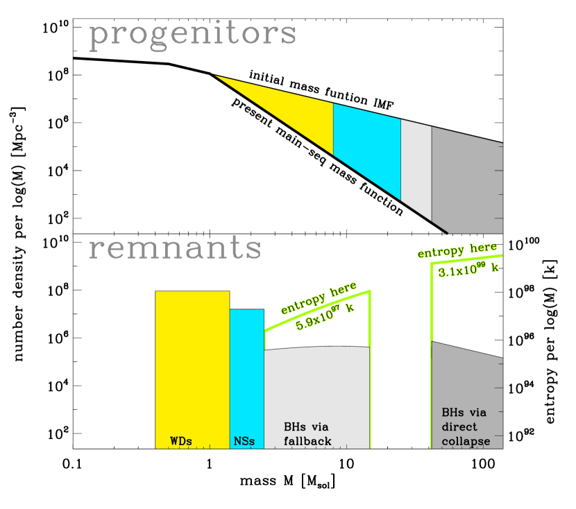
The yellow fill in the top panel represents stars of mass , which died leaving white dwarf remnants of mass (yellow fill, bottom panel). The blue fill represents stars of mass , which died and left neutron star remnants of mass . The light gray area represents stars of mass which became black holes of mass via supernovae (here we use the simplistic final-initial mass function of Fryer and Kalogera (2001)). Stars larger than collapse directly to black holes, without supernovae, and therefore retain most of their mass (dark gray regions; Fryer and Kalogera 2001; Heger et al. 2005).
Integrating Equation (5.3) over stellar black holes in the range (the light gray fill in the bottom panel of Figure 5.3) we find
| (5.34) | |||||
| (5.35) |
which is comparable to previous estimates of the stellar black hole entropy (see Table 5.1). Our uncertainty is dominated by uncertainty in the slope of the IMF, but also includes uncertainty in the normalization of the mass functions and uncertainty in the volume of the observable universe.
If the IMF extends beyond as in Figure 5.3, then these higher mass black holes (the dark gray fill in the bottom panel of Figure 5.3) may contain more entropy than black holes of mass (Equation 5.34). For example, if the Salpeter IMF is reliable to (the Eddington limit and the edge of Figure 5.3), then black holes in the mass range - would contribute about to the entropy of the observable universe. Significantly less is known about this potential population, and should be considered a tentative contribution in Table 5.1.
5.2.7 Supermassive Black Holes
Previous estimates of the SMBH entropy (Penrose, 2004; Frampton et al., 2008; Frampton and Kephart, 2008) have assumed a typical SMBH mass and a number density and yield . Below we use the SMBH mass function as measured recently by Graham et al. (2007). Assuming a three-parameter Schechter function
| (5.36) |
(number density per logarithmic mass interval) they find , , and . The data and best-fit model are shown in black in Figure 5.4.
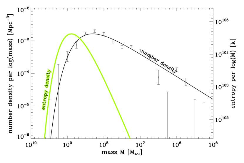
We calculate the SMBH entropy density by integrating Equation (5.3) over the SMBH mass function,
| (5.37) |
The integrand is plotted using a green line in Figure 5.4 showing that the contributions to SMBH entropy are primarily due to black holes around . The SMBH entropy is found to be
| (5.38) | |||||
| (5.39) |
The uncertainty here includes uncertainties in the SMBH mass function and uncertainties in the volume of the observable universe. This is at least an order of magnitude larger than previous estimates (see Table 5.1). The reason for the difference is that the (Graham et al., 2007) SMBH mass function contains larger black holes than assumed in previous estimates.
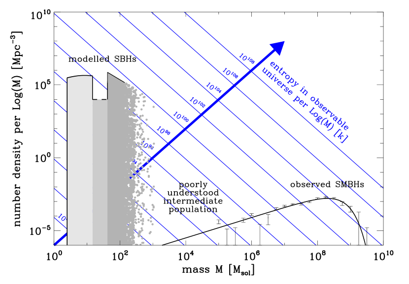
Frampton (2009a, b) has suggested that intermediate mass black holes in galactic halos may contain more entropy than SMBHs in galactic cores. For example, according to the massive astrophysical compact halo object (MACHO) explanation of dark matter, intermediate mass black holes in the mass range - may constitute dark matter. Assuming black holes, these objects would contribute up to to the entropy of the observable universe (Frampton, 2009b). Whether or not this is so depends on the number density and mass distribution of this population. Figure 5.5 combines Figures 5.3 and 5.4 and shows what intermediate black hole number densities would be required.
5.3 The Entropy of the CEH and its Interior
In this section we calculate the entropy budget for scheme 2 (refer to discussion in Section 5.1.1). Scheme 2 differs from scheme 1 in two ways: first, along with the components previously considered (and listed in Table 5.1), here we consider the CEH as an additional entropy component; and second, the volume of interest is that within the event horizon not the particle horizon (or observable universe).
The proper distance to the CEH is generally time-dependent, increasing when the universe is dominated by an energy component with an equation of state (radiation and matter) and remaining constant when the universe is dark energy dominated (assuming a cosmological constant, ). Since our universe is presently entering dark energy domination, the growth of the event horizon has slowed, and it is almost as large now as it will ever become (bottom panel of Figure 5.1). In the Appendix, we calculate the present radius and volume of the CEH
| (5.40) |
| (5.41) | |||||
We also calculate the present entropy of the CEH (following Gibbons and Hawking 1977),
Entropies of the various components within the CEH are calculated using the entropy densities from Section 5.2:
| (5.43) |
Table 5.2 shows that the cosmic event horizon contributes almost orders of magnitude more entropy than the next largest contributor, supermassive black holes.
| Component | Entropy |
|---|---|
| Cosmic Event Horizon | |
| SMBHs | |
| Stellar BHs | |
| Photons | |
| Relic Neutrinos | |
| WIMP Dark Matter | |
| Relic Gravitons | |
| ISM and IGM | |
| Stars | |
| Total | |
| Tentative Components: | |
| Massive Halo BHs | |
| Stellar BHs |
5.4 Discussion
The second law of thermodynamics holds that the entropy of an isolated system increases or remains constant, but does not decrease. This has been applied to the large-scale universe in at least two ways (Equation 5.1 and 5.2). The first scheme requires the entropy in a comoving volume of the universe to not decrease. The second scheme requires the entropy of matter contained within the event horizon, plus the entropy of the event horizon, to not decrease.
We have calculated improved estimates of the current entropy budget under scheme 1 (normalized to the current observable universe) and scheme 2. These are given in Tables 5.1 and 5.2, respectively.
The entropy of dark matter has not been calculated previously. We find that dark matter contributes to the entropy of the observable universe. We note that the neutrino and dark matter estimates do not include an increase due to their infall into gravitational potentials during structure formation. It is not clear to us a priori whether this non-inclusion is significant, but it may be since both components are presently non-relativistic. This should be investigated in future work.
Previous estimates of the relic graviton entropy have assumed that only the known particles participate in the relativistic fluid of the early universe at . In terms of the number of relativistic degrees of freedom, this means at high temperatures. However, additional particles are expected to exist, and thus is expected to become larger as . In the present work, we have calculated the relic graviton entropy corresponding to three high-energy extrapolations of (constant, linear growth and exponential growth) and reported the corresponding graviton temperatures and entropies.
In this paper, we have computed the entropy budget of the observable universe today . Figure 5.6 illustrates the evolution of the entropy budget under scheme 1, i.e., the entropy in a comoving volume (normalized to the current observable universe). For simplicity, we have included only the most important components.
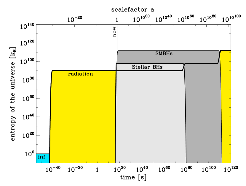
At the far-left of the figure, we show a brief period of inflation. During this period all of the energy is in the inflaton (Guth, 1981; Linde, 1982), which has very few degrees of freedom and low entropy (blue fill; Linde 2009; Steinhardt 2008). Inflation ends with a period of reheating somewhere between the Planck scale () and the GUT scale (), during which the inflaton’s energy is transferred into a relativistic fluid (yellow fill). During reheating, the entropy increases by many orders of magnitude. After reheating, the constitution of the relativistic fluid continues to change, but the changes occur reversibly and do not increase the entropy.
After a few hundred million years (), the first stars form from collapsing clouds of neutral hydrogen and helium. Shortly thereafter the first black holes form. The entropy in stellar black holes (light gray) and SMBHs (dark gray) increases rapidly during galactic evolution. The budget given in Table 5.1 is a snapshot of the entropies at the present time (). Over the next , the growth of structures larger than about will be halted by the acceleration of the universe. Galaxies within superclusters will merge and objects in the outer limits of these objects will be ejected. The final masses of SMBHs will be (Adams and Laughlin, 1997) with the entropy dominated by those with .
Stellar black holes will evaporate away into Hawking radiation in about and SMBHs will follow in . The decrease in black hole entropy is accompanied by a compensating increase in radiation entropy. The thick black line in Figure 5.6 represents the radiation entropy growing as black holes evaporate. The asymptotic future of the entropy budget, under scheme 1, will be radiation dominated.
Figure 5.7 illustrates the evolution of the entropy budget under scheme 2, i.e., the entropy within the CEH, plus the entropy of the CEH.
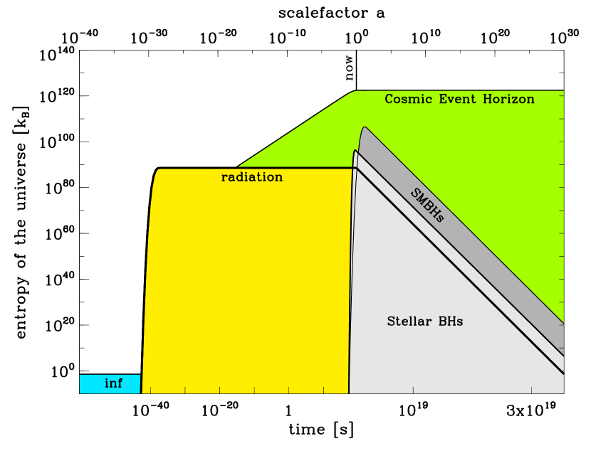
Whereas in scheme 1 we integrate over a constant comoving volume, here the relevant volume is the event horizon. The event horizon is discussed in some detail in the Appendix. During radiation domination, the comoving radius of the CEH is approximately constant (the proper distance grows as ) and in the dark energy dominated future, it is a constant proper distance (). The few logarithmic decades around the present time cannot be described well by either of these.
Since the event horizon has been approximately comoving in the past, the left half of Figure 5.7 is almost the same as in Figure 5.6 except that we have included the event horizon entropy (green fill). The event horizon entropy dominates this budget from about .
After dark energy domination sets in, the CEH becomes a constant proper distance. The expansion of the universe causes comoving objects to recede beyond the CEH. On average, the number of galaxies, black holes, photons etc. within our CEH decreases as . The stellar and SMBH entropy contained within the CEH decreases accordingly (decreasing gray filled regions).
The decreasing black hole entropy (as well as other components not shown) is compensated by the asymptotically growing CEH entropy (demonstrated explicitly for a range of scenarios in Davis et al. 2003), and thus the second law of thermodynamics is satisfied. See Egan and Lineweaver (2010b, in preparation) for further discussion of the time-dependence of the entropy of the universe.
Acknowledgments
We are grateful for many useful discussions with Tamara Davis, Ken Freeman, Pat Scott, Geoff Bicknell, Mike Turner, Andrei Linde, and Paul Steinhardt. C.A.E. thanks Anna Fransson for financial support and the Research School of Astronomy and Astrophysics, Australian National University, for its hospitality during the preparation of this paper.
Appendix: The observable universe and the cosmic event horizon
Here we calculate the radius and volume of the observable universe (for use in Section 5.2); and we calculate the radius, volume, and entropy of the CEH (for use in Section 5.3). We use numerical methods to track the propagation of errors from the cosmological parameters.
The radius of the observable universe (or particle horizon) is
| (5.44) |
Here is the time-dependent scalefactor of the universe given by the Friedmann equation for a flat cosmology
| (5.45) |
Hubble’s constant and the matter density parameter are taken from Seljak et al. (2006): , . The radiation density is calculated from the observed CMB temperature, (Mather et al., 1999), using . The vacuum energy density parameter is determined by flatness, .
A distribution of values is built up by repeatedly evaluating Equation (5.44) at the present time (defined by ) using cosmological parameters randomly selected from the allowed region of parameter space (assuming uncorrelated Gaussian errors in these parameters). We find
| (5.46) |
with an approximately Gaussian distribution. The quoted confidence interval here, and elsewhere in this Appendix, is . The volume of the observable universe is calculated using the normal formula for the volume of a sphere.
| (5.47) | |||||
See Figure 5.8. Uncertainty in and is predominantly due to uncertainty in however also makes a non-negligible contribution.
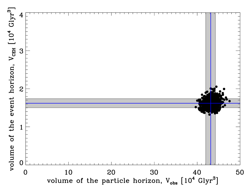
The radius of the CEH at time is given by integrating along a photon’s world line from the time to the infinite future.
| (5.48) |
This integral is finite because the future of the universe is dark energy dominated. Using the same methods as for the observable universe, we find the present radius and volume of the CEH to be
| (5.49) |
and
| (5.50) | |||||
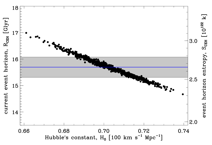
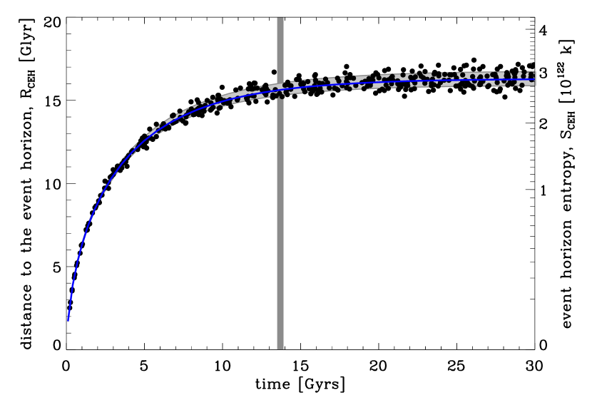
The entropy of the CEH is calculated using the Bekenstein-Hawking horizon entropy equation as suggested by Gibbons and Hawking (1977).
| (5.51) | |||||
Uncertainty in the CEH radius, volume, and entropy are dominated by uncertainties in Hubble’s constant (Figure 5.9).
The CEH monotonically increases, asymptoting to a constant radius and entropy slightly larger than its current value (see Figure 5.10). We calculate the asymptotic radius, volume, and entropy to be
| (5.52) | |||||
| (5.53) | |||||
| (5.54) |
Chapter 6 How High Could the Entropy be and Will the Universe End in a Heat Death?
If we should stay silent,
if fear should win our hearts,
our light will have long diminished,
before it reaches the farthest star.
- VNV Nation, “The Farthest Star”
6.1 Introduction
The increase of entropy (and use of free energy) drives all dissipative physical processes in the universe including gravitational clustering, accretion disks and supernovae, stellar fusion, terrestrial weather, chemical reactions, geological processes and terrestrial-planet-bound biology (Frautschi, 1982; Lineweaver and Egan, 2008).
The long-term sustainability of dissipative processes (including life) depends on the availability of free energy in the future. If, for any reason, the entropy of the universe achieves a value that cannot be further increased, then the universe enters a heat death (see figure 6.1). This idea motivates the exploration of potential entropy growth and entropy limits.
Frampton et al. (2008); Frampton and Kephart (2008) recently estimated that the present entropy of the observable Universe is and that the maximum entropy the universe could have was . Their maximum entropy was calculated by applying the holographic bound (’t Hooft, 1993; Susskind, 1995) to the present volume of the observable Unvierse. That the increase of entropy has not yet been capped by some limiting value is the reason that dissipative processes are ongoing and that life can exist.
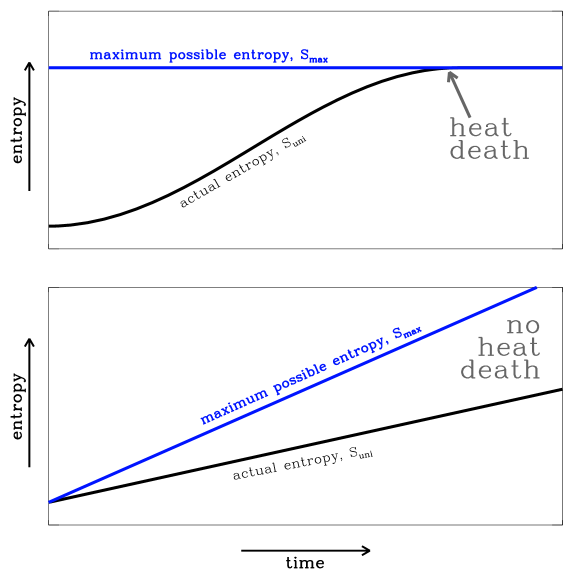
However there remains some ambiguity about how to best define the maximum entropy and whether or not the entropy of the Universe will reach . Figure (6.2) shows several illustrations depicting the relationship between and that have appeared in the literature, books and popular science over the past three decades.
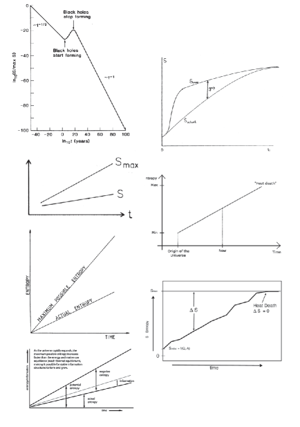
Adams and Laughlin (1997) provide an excellent overview of the processes which, according to our current understanding, will dominate the future evolution of the universe, but in their brief discussion of the thermodynamic fate of a CDM universe (now the standard model of our Universe) they ultimately leave the question of whether our Universe will reach equilibrium, and end in a heat death, open.
More recently (e.g. Bousso et al. 2007; Mersini-Houghton and Adams 2008), the maximum entropy of a de Sitter future has been discussed in the context of anthropic explanations for the low density of the dark energy (the so-called cosmological constant problem), but several issues remain to be clarified.
Below are a number of considerations we have identified to help understand disagreement in the literature. We resolve some, and some deserve further discussion.
-
1.
Theoretically motivated : If is defined using a theoretically motivated entropy bound such as the Bekenstein bound (Bekenstein, 1981) or the holographic bound (’t Hooft, 1993; Susskind, 1995) (both of which apply to weakly gravitating systems) or using the more recent covariant entropy bound Bousso (1999, 2002) (which may apply to strongly gravitating systems), then the result depends on which of these is used.
-
2.
Should we condition on the available energy? In a spherical system of radius which contains mass , the entropy is maximized by converting that energy into massless radiation rather than a black hole (see Page (1981)). The resulting entropy is (in Planck units and dropping constants of order 1) and is much less than the holographic bound (same conventions). This example illustrates that even while theoretically motivated bounds may hold, they are not always the best choice for . If our system is constrained by the amount of energy that is available, then a lower may apply.
-
3.
Should we condition on the equation of state? The energy in a comoving volume is not conserved in an expanding universe (see e.g. (Carroll, 2004)). Generally where is the equation of state, with for radiation, for matter and for dark energy. The amount of energy available at a future time does depend on what form (what ) the energy is stored in. The question of the future of entropy production of the universe therefore depends on whether or not we suppose that energy can be transferred between different equations of state. Harrison (1995) pointed out that energy could be mined from the universe by tethering distant galaxies. A network of tethered galaxies has a negative pressure and an equation of state and is among the scenarios we may be interested in considering in an analysis of possible future entropy production.
-
4.
Normalization volume: Whether the entropy of the universe is increasing or not can depend on the definition of “the Universe”. For example, while the entropy in a comoving volume is constant during adiabatic expansion, the entropy in the observable universe may grow due to the growth of the particle horizon (which bounds the observable universe).
-
5.
How efficiently can energy be collected? If dissipative processes require the collection of matter, then the transport costs (energy and entropy) need to be included in the calculations.
-
6.
Other possible constraints: When asking what the entropy of the universe could be, one is suggesting a universe which is different to the real universe, but has not specified how it is different. Some of the above points, such as “Should we condition on the available energy?” and “Should we condition on the equation of state?” are examples of aspects which are not clearly defined, but there may also be other, more subtle, issues. For example, Frautschi (1982) evaluates during the radiation era by supposing the creation of a large black hole from radiation, but given that mechanisms for this did not exist, the available free energy so calculated have little to do with reality, and may not be of interest.
In the present work we assume an FRW expanding universe with the concordance CDM parameter values, , and (Seljak et al., 2006).
When we say “the entropy of the universe, ” we mean the entropy in the sphere of comoving radius that is now the observable universe. Since the particle horizon grows in comoving coordinates, our comoving sphere was larger than the observable universe in the past and will not include the whole observable universe in the future.
Our aim is to investigate the issues we have listed in this introduction, and others that may arise.
In Section 6.2 we evaluate various entropy bounds that have been proposed in the literature. By applying these bounds on our chosen volume, using a consistent cosmology, we gain some insight into their differences and similarities. In Section 6.3 we explore a natural definition of as the entropy at which the universe has zero free energy given the available energy and exhaust temperatures . The conclusions of these preliminary investigations are also given in Section 6.3.
6.2 Different Versions of
6.2.1 The Holographic Bound
The most discussed entropy bound is the holographic bound (’t Hooft, 1993; Susskind, 1995): the entropy within a sphere of radius will not exceed that of a black hole of radius ,
| (6.1) |
For a comoving volume of physical radius the holographic bound grows as the square of the cosmic scalefactor,
| (6.2) |
and becomes exponentially large in the future.
In figure 6.3 the holographic bound is applied to a sphere of comoving radius (the purple line). The actual entropy in the comoving sphere violates the holographic bound during part the radiation era, as shown in the figure. This occurs because the entropy density of the Universe is approximately homogenous on large scales. The entropy in a volume is whereas the holographic bound grows as the surface area of the volume and for a large enough volume . This violation has been used by Bousso (2002) to motivate a covariant form of the holographic bound. At least in its original form, the holographic bound does not deliver a suitable maximum entropy for the universe.
6.2.2 The Bekenstein Bound
Historically preceding the holographic bound, the Bekenstein bound (Bekenstein, 1981) is the result of a gedankenexperiment in which a package of energy , radius and entropy is deposited into a black hole. The bound,
| (6.3) |
is required by the second law: the entropy lost into the black hole must not be larger than the increase in the horizon entropy of the black hole. Several papers have studied the related effect whereby entropy-containing-matter recedes across the cosmic event horizon to extract similar bounds on the entropy density of matter (Davies, 1987; Bousso, 2001).
The plausibility of the Bekenstein bound was confirmed for numerous weakly gravitating systems (Bekenstein, 2005), but the bound is now known to fail for some gravitationally unstable systems (e.g. Bousso 2002).
In the context of the flat-FRW universe,
| (6.4) | |||||
The Bekenstein bound is constant during the radiation era (when ) and increases during the matter and de Sitter eras ( and respectively). Compared to the Holographic bound, the Bekenstein bound is weaker when applied to regions larger than the Hubble sphere, and stronger when applied to regions smaller than the Hubble sphere. Notice that the Bekenstein bound is not violated in figure 6.3 (the green line).
6.2.3 The Covariant Entropy Bound
A covariant formulation of the Holographic bound was advanced by Bousso (1999): the entropy on convergent light-sheets from a closed surface will not exceed the area of ,
| (6.5) |
In flat spacetime convergent light-sheets from a closed surface cover the entire interior of and the covariant entropy bound (CEB) is the same as the original holographic bound: the entropy interior to cannot exceed the area of . In general spacetimes the convergent light-sheets may not cover the interior of . Specifically, the light sheets may be terminated by a singularity (such as the big bang) or they may stop converging and start to diverge (in which case they are truncated). In both of these cases the light sheets only cover part of the interior of and the CEB is weaker than the corresponding holographic bound.
We calculate the covariant entropy bound in an expanding, flat, FRW universe by choosing the surface and light-sheet such that the entropy density bound on the light-sheets is strongest (following the prescription given in Bousso (1999)). We find that the strongest bound on the comoving entropy density comes from the past-outgoing lightsheet of a closed spherical surface with a radius infinitessimaly larger than . In this case the comoving entropy density is limited to
| (6.6) |
where is the conformal time. The dark blue line in figure 6.4 shows this bound applied to a sphere of comoving radius , i.e.
| (6.7) |
The bound is saturated by the entropy of radiation fields at the Planck time, increases during radiation and matter domination, and asymptotes to a constant during the de Sitter future,
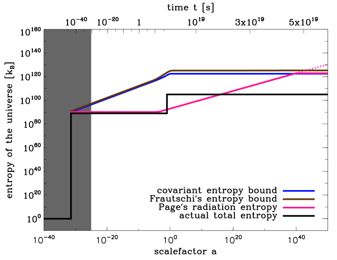
6.2.4 Frautschi’s Maximum Entropy
Frautschi (1982) identifies the maximum entropy inside a causal region (particle horizon) as the entropy produced by the collection of all matter into a single black hole.
Following Frautschi (1982), the mass available in any causal region for the formation of the black hole is
| (6.9) |
where is the comoving radius of the particle horizon. The corresponding entropy is
| (6.10) | |||||
We are interested in the total entropy in a comoving volume of radius . In the early universe this comoving volume contains many adjacent particle horizons, each with potentially . The corresponding maximum entropy for a comoving volume is thus
| (6.11) | |||||
The brown line in figure 6.4 applies this bound to a sphere of comoving radius . During radiation domination and so the limit on grows as . During matter domination and so the limit on grows as . During vacuum domination (but assuming black holes cannot be made from dark energy), and so the limit on is .
The possibility of limited gravitational clustering was acknowledged by Frautschi (1982), but in the closed cosmology of the day his work on led him and others to favor increasingly instability. The same idea, as presented here with updated cosmology, now predicts stability and a constant .
Note that the qualitative future of depends strongly on whether or not black holes can be made from dark energy. If we include the dark energy, then and so the limit on grows as (not shown in figure 6.4).
Since black holes may radiate via the Hawking process they do not generally represent the maximum entropy state Page and McKee (1981); Frautschi (1982), i.e. it may be the case that Frautschi’s bound is not only attainable (it is that by construction), but in sufficiently empty universes it will be surpassed by the evaporation of black holes. This is explored in the next section.
We note that Frautschi’s idea may be unreliable in recent times. After matter domination, the black holes suggested in equation 6.9 have radii larger than the Hubble sphere and are not Schwarzschild black holes. Further work on the interaction between large black holes and the FRW universe is needed to understand the entropy in such situations.
6.2.5 Page’s Evaporated Matter
Stellar black holes (with masses ) and SMBHs at the center of galaxies (with masses ) emit Hawking radiation with characteristic temperatures of and respectively. Both these temperatures are far below that of the present CMB () and consequently both classes of BHs currently absorb more radiation than they emit. As the universe is starting to grow at an exponential rate, the CMB will be quickly redshifted below the temperatures of these black holes. should come when the universe is old and when it is .
By the time black holes stop growing by accretion, the background temperature of the universe will be lower than the temperature of any black holes. They will begin to evaporate. The formation of cluster-sized SMBHs up to is expected (see e.g. (Frampton and Kephart, 2008)). Subsequent evolution will depend on the Hawking process. Black holes this large will have temperatures of , which will be hotter than the background after the universe is just old.
It may be possible in principle to transmute matter in the universe into radiation via black hole evaporation. In principle this could be done locally everywhere, in an arbitrarily short time, by using sufficiently small black holes. After evaporation, further entropy could be produced by re-thermalizing the Hawking radiation (e.g. by scattering off trace particles). The immediate transmutation and re-thermalization of all radiation, baryons and dark matter would result in a new blackbody background with temperature
| (6.12) |
and entropy
| (6.13) | |||||
This was identified by Page and McKee (1981) as an upper limit to the entropy of the universe. Since decreases less quickly than more entropy is produced per comoving volume if the transmutation and re-thermalization is done later rather than sooner. Page and McKee (1981) suggested that the entropy in a comoving region of the universe could be made arbitrarily large in this way.
The orange line in figure 6.4 shows the entropy produced by the immediate transmutation and re-thermalization of all radiation, baryons and dark matter in the universe. The current maximum entropy of the universe calculated in this way is
| (6.14) |
This is much lower than the actual current entropy (; Egan and Lineweaver 2010a). This is because BHs and SMBHs are much colder than the CMB; in environments as hot as the present universe BHs and SMBHs do not spontaneously evaporate.
6.2.6 Page’s Evaporated Matter - de Sitter Limited
A minor adjustment of Page’s idea is required in the presence of a de Sitter cosmic horizon. At the temperature in equation 6.12 falls below the de Sitter temperature . However, the de Sitter radiation would prevent any (re-)emission of radiation at temperatures lower than .
Thus the final minimum temperature of the evaporated black hole radiation is
| (6.15) |
and the entropy density is
| (6.16) |
Figure 6.4 shows this entropy bound applied to a sphere of comoving radius (the dotted orange line). Since the density tends to decay as in late times, the maximum entropy in a comoving volume tends to a constant.
6.3 Discussion
The definition of “the universe” as a comoving volume is a practical answer to issue 4. We have not checked whether using this definition reveals any more or less than if we had defined the universe to be the region within the particle horizon (i.e. the time-dependent observable universe), or the event horizon.
Our interest in the entropy history is primarily driven by the question of the long-term sustainability of dissipative processes including life. These processes depend on the availability of free energy (not energy). Dissipative processes deplete free energy by degrading an amount of high-grade (low entropy) energy into an equivalent amount of low-grade (high entropy) energy. As an example of this, dissipative weather action diffuses high-grade energy received from the Sun ( photons) into low-grade energy which is re-transmitted to space ( times as many photons at ) (Lineweaver and Egan, 2008).
6.3.1 Free Energy and an Defined by Zero Free Energy
Consider a system with total energy and entropy , which is connected via a heat engine to an infinite exhaust bath at temperature . The system, which is used to fuel the engine has free energy
| (6.17) |
which is generally less than its total energy. That is to say, the engine may extract all but of the energy. The unextractable energy is necessarily expelled as exhaust and guarantees that the entropy of products is at least as large as the entropy of the consumed fuel.
| (6.18) |
For real systems the exhaust bath may not be infinite and the temperature may not be constant. In this case 6.17 should be replaced by an integral equation.
The most natural definition of is one at which the system has zero free energy.
| (6.19) | |||||
The universe is not in a heat death today because (and so ). Nevertheless, the amount of energy in a comoving volume, and the minimum available exhaust temperature , are both finite and so there is some finite entropy which, if today, there would presently be no free energy.
means that no free energy is available, but it does not mean that no free energy can become available. Both quantities on the right-hand-side of equation 6.19 potentially change with time. Figure 6.5 shows the evolution of (thick black; taken to be energy in radiation and matter in a comoving volume) and three potential exhaust temperatures,
| (6.23) |
The first potential exhaust that we have considered is the cosmic microwave background (CMB; shown in green), the second are large black holes (the largest causal black hole is shown in thick pink; refer to Section 6.2.4), and the third potential exhaust is the the de Sitter background (thick purple).
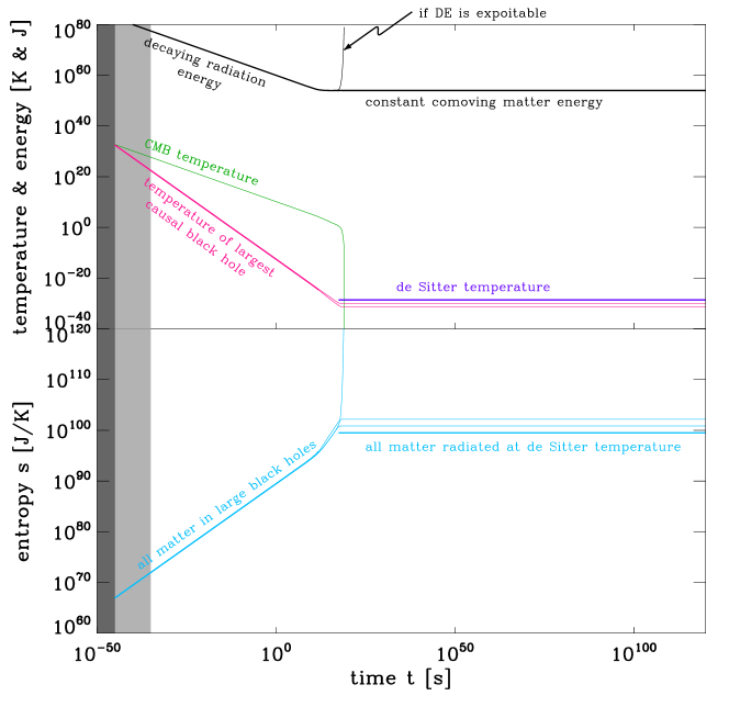
Today the lowest available exhaust temperature is that of a large black hole (not that of the CMB). If we suppose that large causal black holes could have existed during the radiation era, then those black holes would have been the lowest available exhausts then, and dissipative processes might have been driven by the CMB-black hole temperature gradient. In the near future the CMB temperature will drop below the de Sitter temperature, and that will become the lowest available exhaust.
The maximum entropy is calculated using equation 6.19 and is shown in thick blue in the bottom panel of Figure 6.5. Since and become constant in the future, and the entropy within the considered comoving volume can only increase, the amount of free energy in the comoving volume decreases in the future (see equation 6.17).
The that we have discussed in this section is defined in terms of the available energy and exhaust temperatures (equation 6.19). It is quantitatively similar to the maximum entropy of Frautschi (1982, 1988) by construction (see Section 6.2.4). It is also quantitatively similar to the covariant entropy bound of Bousso (1999) (applied to the same volume; see Section 6.2.3), although the reason for this is not clear to us.
In this section we used the conserved matter in a comoving volume and the constant de Sitter temperature to show that maximum entropy in the comoving volume becomes approximately constant in the future. The bleak implication for dissipative processes is that there is a finite amount of free energy in any comoving volume. On the other hand, the fraction of that is not free (due to the cumulative increase in entropy to the present day) is only
| (6.24) |
As mentioned in the introduction (issue 3) future entropy production may depend on whether or not the equation of state of matter can be changed. Using figure 6.5 it is easy now to see the effect this might have. If energy was converted from matter into a form with a lower equation of state then the energy (the black line in Figure 6.5) would increase into the future instead of becoming constant. The exhaust temperature (de Sitter temperature) would not change significantly, since it depends primarily on the dark energy density. As a consequence the maximum entropy, and the free energy would increase. On the other hand, if matter were converted into a form with (such as radiation, ) would cause to decrease into the future. Again, remains unchanged and and and would decrease with time.
Chapter 7 Conclusions
As the music finishes again,
have you thought about,
how we almost never lift our eyes,
from the ground,
to the black space above the clouds.
- Kent, “View From a Castle in the Sky”
The Cosmic Coincidence Problem
Matter and dark energy are observed to presently contribute to the total cosmic energy density in the ratio
| (7.1) |
Since the matter and dark energy densities dilute at different rates during the expansion of the Universe, we are faced with the cosmic coincidence problem: Why are the current matter and dark energy densities the same order of magnitude today? In other words, why is (as defined above), so large?
We have used the temporal distribution of terrestrial planets in the Universe to estimate the temporal range during which terrestrial-planet-bound observers are likely to arise. Using this observer distribution we have quantified the severity of the cosmic coincidence problem by computing the probability of observing values of larger than .
Assuming the standard CDM density histories for and we find
| (7.2) |
Given the temporal distribution of terrestrial planets, terrestrial-planet-bound observers have a large probability of observing the matter and dark energy densities to be at least as close as we measure them to be.
The same method is applied under the assumption of dynamic dark energy, with an equation of state parameterized by and . We find that some regions of - parameter space can be discriminated against on grounds of the coincidence problem. I.e. for some regions of - parameter space, the probability of observing values of is very low (Figure 3.7). However those regions are already strongly excluded by observations.
Our main result is an understanding of the coincidence problem as a temporal selection effect if observers emerge preferentially on terrestrial planets which is found to hold under any model of dark energy fitting current observational constraints. The cosmic coincidence problem is therefore removed as a factor motivating dark energy models.
Searching for Life Tracers Amongst the Solar Properties
We have compared the Sun to representative stellar samples in properties. The properties were selected based a plausible relation to life, availability of a representative stellar sample for comparison, and such that they were maximally uncorrelated. No properties were added to, or removed from the analysis based on previous information about whether or not the Sun was anomalous in those properties.
Those selected properties were
-
1.
mass,
-
2.
age,
-
3.
metallicity,
-
4.
carbon-to-oxygen ratio,
-
5.
magnesium-to-silicon ratio,
-
6.
rotational velocity,
-
7.
galactic orbital eccentricity,
-
8.
maximum height above galactic plane,
-
9.
mean galactocentric radius,
-
10.
host galaxy mass and
-
11.
host group mass.
Our main results are:
-
•
Mass and galactic orbital eccentricity are the most anomalous properties of those included in our study. The Sun is more massive than of nearby stars and has a Galactic orbit which is more circular than of FGK stars within .
-
•
When the parameters are considered together, the probability of selecting a star, at random, which is more anomalous than the Sun, is just .
The observed “anomalies” in mass and galactic orbital eccentricity are consistent with statistical noise (refer to Figure 4.4). This contrasts with previous work suggesting anthropic explanations for the Sun’s high mass.
To our knowledge, this is the most comprehensive comparison of the Sun to other stars.
The Entropy of the Present and Future Universe
We present budgets of the entropy of the observable Universe (Table 5.1) and of the cosmic event horizon and its interior (Table 5.2). To our knowledge these are the most comprehensive and quantitative budgets of the present entropy of the Universe. The components included are
-
1.
the cosmic event horizon (only applicable to the latter budget),
-
2.
supermassive black holes,
-
3.
tentative stellar black holes in the range -,
-
4.
confirmed stellar black holes in the range -,
-
5.
photons,
-
6.
relic neutrinos,
-
7.
dark matter,
-
8.
relic gravitons,
-
9.
interstellar and intergalactic media and
-
10.
stars.
The present entropy of the observable universe is found to be
| (7.3) |
and is dominated by supermassive black holes. This is to be compared with previous estimates in the range to . Our larger value arises from the inclusion of a new measurement of the supermassive black hole mass function.
The present entropy of the cosmic event horizon is calculated to be
| (7.4) |
dwarfing that of its interior,
| (7.5) |
Figure 5.5 illustrates the possible role played by intermediate mass black holes. The time evolution of these two budgets is discussed (see Section 5.4 and Figures 5.6 and 5.7).
Entropy bounds from the literature are applied to a comoving volume normalized to the present observable Universe (Fgures 6.3 and 6.4). While the Bekenstein bound and the holographic bound become arbitrarily large, Bousso’s covariant entropy bound on this volume increases monotonically and asymptotes to a constant around . As does a simplistic bound based on the assumption that the comoving matter density is constant and that the future background temperature is the de Sitter temperature. According to both of these bounds the free energy in the comoving volume is also finite and a heat death is therefore expected (either in a finite time or asymptotically).
Appendices
Appendix A Entropy and the Free Energy Prerequisites for Life in the Universe
Charles H. Lineweaver
Chas A. Egan
A.1 The Irreversible History of Entropy
A.1.1 Pedagogical Pitfalls
Although an undergraduate education in the physical sciences contains no explicit warnings against thinking about biology, most physics graduates come out believing that the most fundamental aspects of the universe are dead things in equilibrium obeying conservative forces. Frictionless pendulums may be simple, but when studied for too long, students begin to believe that they really exist. They don’t. Friction is not just an optional accessory inserted into simple equations to make life difficult. Friction, dissipation and the unequal sign in the second law of thermodynamics is what makes life possible. The first law of thermodynamics (energy conservation) precedes the second (entropy increase) in textbooks, but there is no evidence that this precedence reflects any natural order of things in the universe.
Physicists are taught that whatever biology is about, it can be reduced to chemistry; and that whatever the chemists are up to, it can be reduced to physics. However, physics as we know it can also be viewed as a subset of biology since all physicists are the products of biological evolution.
Much has been made of our current inability to unify general relativity and quantum mechanics to arrive at a theory of everything. Although the murky relationship between gravity and entropy may provide key insights into the theory of everything, it has received much less attention. Although gravitational collapse plays the most important role in converting the initial low entropy of the universe into the dissipative structures we see all around us (including ourselves), gravity is almost universally ignored in thermodynamics textbooks.
“We do not yet know if the second law applies to gravitational interactions. Is the second law valid only from a given (or “slowly” varying) gravitational state? Can we include gravitation?” (Prigogine 1980, p. 196)
In this paper, we attempt to make sense out of the relationship between life, gravity and the second law of thermodynamics. In Section A.1 we briefly review the history of attempts by physicists to understand life. In Section A.2 we describe how free energy and low entropy radiation from the Sun maintains the low entropy structures of Earth. We review the entropy of photons in an expanding universe in Section A.3 and consider the relationship between gravity and entropy in Section A.4. We conclude by discussing the heat death of the universe (Section A.5). Our goal is to understand more clearly how gravitational collapse is the source of free energy for life in the universe. Appendices contain mathematical details.
A.1.2 Physicists and Life
When iconoclastic physicists move out of equilibrium and think generally about the question “What is life?”, the concepts of entropy and free energy play central roles. In the first half of the 19th century, Carnot(1824), Clausius(1867) and others came to understand that although energy is conserved and can not be destroyed, useful work – or extractable free energy – could be destroyed. Irreversible processes are destroying free energy all the time. Ludwig Boltzmann (1886) was concerned about entropy and the distinction between energy and free energy:
“The general struggle for existence of animate beings is therefore not a struggle for raw materials — these, for organisms, are air, water and soil all abundantly available – nor for energy which exists in plenty in any body in the form of heat (albeit unfortunately not transformable), but a struggle for entropy, which becomes available through the transition of energy from the hot sun to the cold earth.”
In Section A.2 we describe and quantify this “transition of energy from the hot sun to the cold earth”. Although Boltzmann explicitly talks about “animate beings”, the same thing could be said about any far from equilibrium dissipative structure: convection cells, hurricanes, eddies, vortices and accretion disks around black holes (Glansdorff & Pirgogine 1971, Nicolis & Prigogine 1977, Prigogine 1980). Life is a subset of this general class of dissipative structure (Schneider & Kay 1994, 1995, Lineweaver 2006, Schneider & Sagan 2006).
In “What is Life?” (Schroedinger 1944) made it clear that Boltzmann’s animate beings were not struggling for entropy. If they were struggling at all, it was to get rid of entropy, or to absorb negentropy:
“What an organism feeds upon is negative entropy. Or, to put it less paradoxically, the essential thing in metabolism is that the organism succeeds in freeing itself from all the entropy it cannot help producing while alive.”
In the notes for a later edition (1956) Schroedinger apologizes to his physicist colleagues and admits that instead of negative entropy, he should have been talking about free energy. There is general agreement that life on Earth (and elsewhere) depends on the non-equilibrium of the universe and requires free energy to live.
“[T]he one unequivocal thing we know about life is that it always dissipates energy and creates entropy in order to maintain its structure.” (Andersen and Stein 1987).
In our search for extraterrestrial life, we can use the most fundamental aspects of terrestrial life to guide us. At the top of the list is life’s requirement for free energy. Despite uncertainties in the temperature limits of life ( C?), despite uncertainties in which solvent life can use (water?), despite uncertainties in its chemistry (carbon-based?) - extraterrestrial life, like terrestrial life, will need a source of free energy. Free energy is a more basic requirement that all life anywhere must have. Thus, instead of “follow the water”, our most fundamental life-detection strategy should be “follow the free energy”. To find chemistry-based life we should look for the redox gradients between electron donors and acceptors. These considerations motivate us to quantify and understand the origin of free energy (Fig. A.1).
In the beginning, 13.7 billion years ago, the universe was very hot. There was no life and there were no structures in the universe. The universe was a thermal heat bath of photons and a soup of nuclei (and later atoms) in chemical equilibrium. Life is not possible in such an environment. In thermal equilibrium and chemical equilibrium, no free energy is available. As the universe expanded, the heat bath cooled and life emerged. Life did not emerge simply because the universe cooled down to have the right temperature for to be a liquid. Life needed a source of free energy unavailable from an environment in chemical and thermal equilibrium. In this paper we try to clarify the idea that the origin of all sources of free energy can be traced back to the initial low gravitational entropy of the unclumped matter in the universe (e.g. Penrose 2004). The gravitational collapse of this matter produced galaxies, stars and planets and is the source of all dissipative structures and activities, including life in the universe. See Dyson (1979), Zotin (1984) and Chaisson (2001) for discussion of how life (unlike abiotic dissipative structures) seems to evolve toward more complexity.
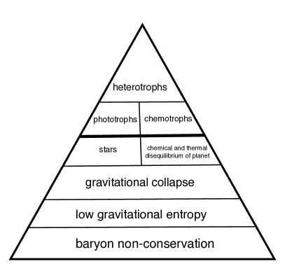
A.1.3 The Pyramid of Free Energy Production
Usually bacteria are considered to be at the bottom of the food chain or at the base of the primary production pyramid, but an interesting perspective comes when we add layers to the base of the pyramid. At the top of Fig. A.1 are heterotrophs, who eat (= extract free energy from ) organic compounds (including other heterotrophs) produced by the primary producers one level down. Heterotrophs include wolfs, humans, fish and mushrooms. Supporting all heterotrophic life are the primary producers (phototrophs and chemotrophs). Although phototrophs and chemotrophs are usually considered to be primary producers, they get their free energy from solar photons and inorganic compounds, respectively. Phototrophs include plants and cyanobacteria and all photosynthesizers. Chemotrophs include iron and manganese oxidizing bacteria living off the non-equilibrium chemistry of igneous lava rock.
The vertical line in Fig. A.1 indicates that stars are the free energy sources for phototrophs while the chemical and thermal disequilibrium of the Earth is the source of the free energy in the inorganic compounds used in the metabolisms of chemotrophs. The source of both the free energy provided by stars and by planets comes from gravitational collapse in the level below in the sense that the source of starlight is the fusion reactions taking place in the hot, dense center of the Sun that is the result of gravitational collapse. The chemical and thermal disequilibrium of the Earth also has its source in the free energy of gravitational collapse.
Moving one level lower in the pyramid, gravitational collapse is made possible by an initially very diffuse, almost unclumped distribution of baryons. Unclumped baryons in the early universe provided the initial low entropy of the universe. At the lowest level in the pyramid, the source of these almost unclumped baryons is baryon non-conservation (Sakharov 1967). The low initial gravitational entropy of the universe and baryon non-conservation are discussed further in Section A.4.
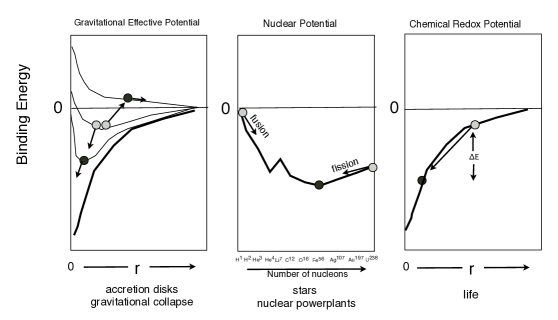
The sources of free energy in the universe are summarized in Fig. A.2. In a gravitational system (left panel), such as a protoplanetary accretion disk, consider a small mass in orbit at distance from a large mass at . The effective potential, including angular momentum is (e.g. Goldstein 1980). Angular momentum must be reduced for gravitational collapse to happen. Consider two small masses, originally in identical effective potentials (two light grey balls). They come close to each other and exchange some angular momentum. The one that lost , sinks into the well closer to , the one that gained distances itself from . Since the of each mass has changed, their effective potentials have diverged. One collapses, the other is expelled. Without the dissipation of energy, expulsion of matter and transfer of angular momentum that occurs in the turbulence and viscosity of an accretion disk (e.g. Balbus 2003), matter would not gravitationally collapse. The efficiency of star formation in a molecular cloud is a few percent. A substantial fraction of the infalling matter is scattered, or receives a large dose of angular momentum as it is processed through the accretion disk and then expelled (Balbus 2003). Therefore accretion disks are also expulsion disks (see Fig. A.3 for the role of dynamical friction in the gravitational collapse of less-viscous non-accretionary systems). Gravitational collapse creates entropy by radiating away the potential energy and expelling high velocity, high angular momentum material.
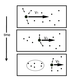
Fusion in the core of the Sun was made possible by the gravitational collapse of kg of hydrogen resulting in high densities and temperatures. Gravitational collapse also provides the conditions in the cores of stars to make matter roll down the nuclear binding energy curve to the energy minimum (middle panel, Fig. A.2).
The right panel of Fig. A.2 shows that the amount of energy extractable from chemical bonds depends on the energy difference between the electron in the potential well of the donor and that of the acceptor (Nealson & Conrad 1999). Life takes in energy-rich atoms with electrons in high orbitals (electron donors) and excretes the same atoms with the electrons in the deeper atomic or molecular orbitals of electron acceptors. Solar photons provide the energetic kick to lift the electrons back up during photosynthesis in phototrophs, who provide the energy-rich materials for heterotrophs (e.g. Szent-Gyorgi 1961).
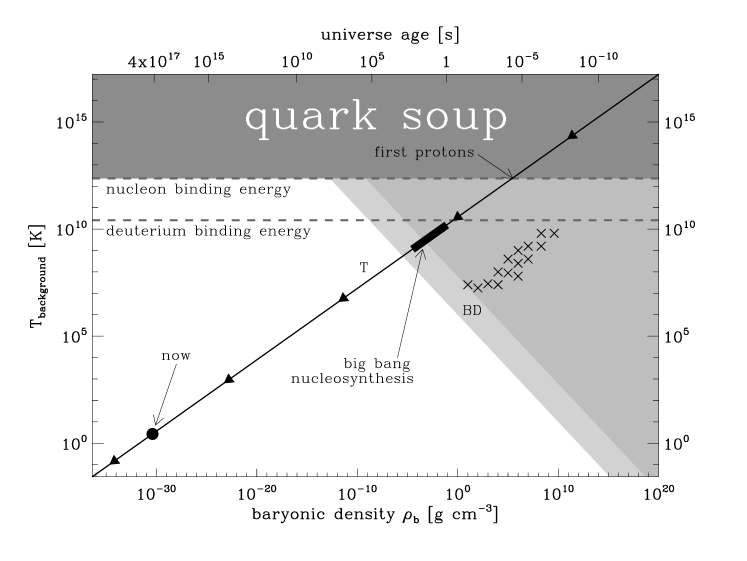
A.1.4 Big Bang Nucleosynthesis and the Subsequent Low Entropy of Nuclei
As the universe expands, the scale factor increases, the temperature decreases () and the density decreases . Thus, . This is the path the universe takes in Fig. A.4 starting at some initial temperature and density: . The early universe expanded and cooled too quickly for big bang nucleosynthesis to fuse hydrogen into iron and reach equilibrium at the lowest nuclear binding energy per nucleon (middle panel, Fig. A.2). Thus, big bang nucleosynthesis left nuclei in a low entropy, high energy state. Similarly, reheating after inflation (Kolb & Turner 1990) left unclumped baryons in a state of low gravitational entropy since the baryons are not at the bottom of the gravitational potential wells.
Entropy is produced when free energy is extracted from the sources of potential energy shown in Fig. A.2. For example, dissipation of gravitational energy (left panel) happens when the turbulent viscosity and friction of an accretion disk transfers angular momentum away from the central mass and makes some material fall onto the central mass while other material is expelled. Without such collisions, turbulence and friction, angular momentum would not be transferred and material would not gravitationally collapse or be expelled. Figure A.8 illustrates gravitational systems with minimal dissipation.
Dissipation happens and entropy is produced whenever a photon gets absorbed by a material at a temperature colder than the emission temperature. The photon energy gets reemitted and distributed among many photons. This happens as a gamma ray produced by fusion at the center of the Sun makes its way to the photosphere where its energy is distributed among millions of photons (Frautschi 1988). It also happens when the energy of solar photons ( K) are harvested for photosynthesis by plants at temperatures below K, and when the Earth reemits solar energy at infrared wavelengths.
Energy cannot be created or destroyed. Therefore, strictly speaking, we cannot “use energy” or “waste energy”. Energy can however be degraded. Low-entropy, high-grade energy dissipates into high-entropy, low-grade energy. Life does not “use” energy since the same amount of energy that enters the biosphere, leaves the biosphere. Life needs a source of free energy, and is unable to use high entropy energy. Life takes in energy at low entropy and excretes it at high entropy. Any engine does the same thing. When coal burns, energy is conserved. Electrons are high in the electric potentials of the fuel and lower in the potentials of the ashes and exhaust gases. The difference ( in the right panel of Fig. A.2) has been transfered into heat and work.
Two types of free energy are described in the literature: Gibbs free energy and Helmholtz free energy (e.g. Sears & Salinger 1975). For simplicity and convenience (cf. Appendix A) we focus on the Helmholtz free energy of a system:
| (A.1) |
where is the internal energy of the system, is its temperature and is its entropy. The free energy , is the amount of energy that can be extracted from the system to do any kind of useful work such as climbing a tree or assembling fat molecules. Equation A.1 shows that all of the internal energy is not available to be extracted as free energy . There is an entropic tax: . is the penalty one must pay for extracting the energy from the system and using it to do any useful work. is how much money is in the bank and are the bank fees you have to pay to get it out. The higher the temperature and the higher the entropy of the system, the higher the penalty and the lower will be the extractable, usable, life-supporting, life-giving free energy . Good engines produce minimal entropy and have and thus (Bejan 2006, Eq. 3.7).
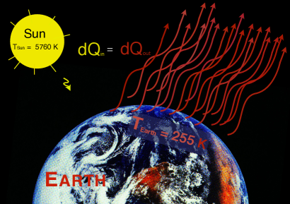
A.2 The Sun is the Source of Earth’s Free Energy
Consider the amount of free energy that is delivered to the Earth in solar photons. We make the reasonable assumption that the Earth is in a steady state (e.g. Kleidon 2008). It is not in equilibrium because there is an energy flow in to the system (sunlight) and out of the system (Earth radiates to space, Fig. A.5).
Steady state means that the average effective temperature of the Earth is constant. It also means that the amount of energy delivered to the Earth in solar photons , is the same as the amount of energy radiated away by the Earth as infrared photons, . Thus, . If this were not so, the internal energy of the Earth would be increasing – the Earth would be getting hotter or the speed of winds and the number of hurricanes would increase, or there would be a net increase in biomass. However, the number of organisms that are born is about the same as the number that die. The strength of the winds that dissipate the pole to equator temperature gradients are about the same and the number of hurricanes which equilibrate thermal, pressure and humidity gradients, is about the same. (We are ignoring variations in the temperature of the Earth due to variations of the greenhouse gas content of the Earth or the Milankovich cyles or the secular increase in solar luminosity.) Thus, in steady state, the Earth is at a constant temperature , constant energy , constant entropy and constant free energy .
Let be all the entropy produced by all the dissipative structures on Earth (including winds, hurricanes, ocean currents, life forms, and the thermal dissipation when heat is transfered through the soil from hot sunny spots to cool shady spots). Then we have for the entropy of the Earth:
| (A.2) |
or the net decrease in entropy from photons coming in and out () is compensated for by the increase in entropy from all the dissipative, low entropy structures on Earth. Thus,
| (A.3) |
Since the energy in the photons arriving and leaving is equal, , we have since:
| (A.4) | |||||
| (A.5) |
Thus,
| (A.6) |
Thus, the Earth exports twenty times as much entropy as it receives. Equation (A.27) then tells us that the ratio of the number of emitted photons to the number of absorbed photons is:
| (A.7) |
This is shown in Fig. A.5 with its 1 incoming solar photon and 20 outgoing infrared photons. The entropy flux to and from the Earth from the absorbtion of solar photons and the emission of infrared photons is:
| (A.8) | |||||
Since the amount of free energy is not building up in the Earth, we have . Let be the amount of free energy delivered to the Earth by solar photons and be the amount of free energy dissipated by all the dissipative structures on Earth, then (cf. Eqs. A.2 and A.3) we have,
| (A.9) |
or
| (A.10) |
where the minus sign indicates that is the loss or dissipation of free energy. Eqs. (A.9) and (A.10) are the key to understanding how the Earth can keep absorbing free energy from the Sun without the amount of free energy in the Earth going up. The free energy in the food we eat goes to cell repair and movement, and is dissipated when we die or move. Similarly, all of the free energy delivered by the Sun is dissipated in winds, hurricanes, ocean currents, life forms, or thermal conduction through soil between sunny spots and shady spots.
The Earth is exporting much entropy but the entropy of the Earth is not decreasing. That is because the dissipative structures on the Earth are producing the entropy that is exported. They need the input of free energy to stay at low entropy – just as a refridgerator needs free energy to stay at a constant low temperature (= low entropy steady state). Without a supply of free energy a fridge will heat up, a hot water tank will cool down, and life will die. Things approach equilibrium. It takes free energy to keep a fridge cool, the tank hot and the chemical order in life forms. Free energy (or work) is needed to remove the heat and entropy that naturally leaks into the fridge. The lower the temperature of the fridge and the more imperfect the insulation, the more free energy is needed to maintain the low entropy steady state.
The export of entropy does not lower the entropy of the Earth. Rather it keeps the entropy of the Earth at a constant low level. In the absence of a flow of negentropy, the low entropy structures, such as hurricanes, dust devils, the hydrological cycle, thermal gradients and life forms would run down and dissipate away. The export of entropy compensates for this natural dissipation and is the reason why low entropy structures endure.
A.2.1 How much entropy is produced and how much free energy can be extracted from a solar photon?
We can compute the amount of free energy available on the Earth to drive the winds, hurricanes and all of life (Kleidon 2008). Starting from Eq. A.1, taking differentials and then dividing by yields the rate of increase of free energy of the Earth:
| (A.11) |
Since we are assuming steady state, F, U, T and S are all constants and all of the terms in Eq. A.11 are zero. However, using Eqs. (A.2) and (A.9) we can write:
| (A.12) |
Separating terms to count only the contribution from photons we get:
| (A.13) |
With Eq. A.8 this yields,
| (A.14) |
Thus, of the incoming solar energy can be used to do work, i.e. photovoltaics at the temperature of the Earth have a maximum efficiency of . To get a numerical value for the free energy in Eq. (A.14): the solar flux impinging on the disk of the Earth () at 1 AU from the Sun is . Since , the average flux from the Earth’s surface () balances the solar flux:
| (A.15) |
where, .
Therefore, to get a numerical value for (= the flux density of solar radiation through a unit area of ) we have:
| (A.17) |
where is the albedo of the Earth, and the Stefan-Boltzmann constant is . Thus the flux of free energy through unit area (Eq. A.14) is
| (A.18) |
This flux of free energy maintains all thermal gradients on the surface of the Earth, all winds and hurricanes and all life, and is equal to the flux of free energy that is dissipated by all dissipative structures (Eq. A.10).
The total free energy available from sunlight is the flux per unit area times the area of the Earth: W, which is about ten thousand times larger than the W of global power consumption from burning fossil fuels. Terrestrial life (including humans) is a subdominant dissipator of the free energy delivered to Earth (Kleidon 2008).
There are no hurricanes or ocean currents on the Moon, so how does the free energy delivered by solar photons get dissipated there? Performing the same computation for the Moon as we did for the Earth we have:
| (A.19) |
where the Moon’s albedo is lower than the Earth’s, (). The Moon’s effective temperature is higher than the Earth’s because of the Moon’s lower albedo. Instead of having hurricanes, winds, ocean currents and life forms, the free energy of the Moon is dissipated by heat flow due to the large temperature gradients (low entropy structures) between regolith in the sunshine at K and the shadows at K. The input of low entropy solar radiation maintains the gradients. The maximum temperature variation on the Moon is K between K at the equator in the early afternoon and K in the shade at the poles. On Earth, this variation is only K between K and K. If the Moon were the same temperature as the Sun, K then the “shadows” would be the same temperature as the Sun and there would be no export of entropy. If the Moon were a smooth ball instead of having a bumpy surface then the large scale hemispheric temperature gradient would be the only low entropy structure and a larger temperature gradient would be created to dissipate the same constant amount of free energy from the low entropy photons. A further refinement to the computation above would consider the low entropy associated with sunlight coming from a particular direction rather than isotropically.
A.3 The Entropy of the Cosmic Microwave Background Remains Constant as the Universe Expands
It is difficult to talk about the total entropy in the universe without knowing how big the universe is, so we talk about the entropy in a representative sample of the expanding universe. Typically we put an imaginary sphere around a few thousand galaxies and consider the entropy in this expanding sphere – the entropy per comoving volume. We parameterize the expansion of the universe with a scale factor R. This means that when the universe increases in size by a given factor, R increases by the same factor (Fig. A.6).
The expansion of the universe is adiabatic since the photons in any arbitrary volume of the universe have the same temperature as the surrounding volume. There is no net flow of heat. The entropy of a photon gas does not increase under adiabatic expansion. Specifically, the entropy of a gas of photons in a volume at temperature is (e.g. Eq. A.23 or Bejan 2006, eq. 9.20).
The photon wavelengths , increase (are redshifted) with the scale factor: . There is no absorbtion or reemission associated with the redshifting of cosmic microwave background photons. These photons were last scattered at the surface of last scattering years after the big bang. Since the volume increases as , and since the temperature of the microwave background goes down as the universe expands: , we have the result that the entropy of a given comoving volume of space is constant (Kolb & Turner 1990, Frautshi 1982, 1988):
| (A.20) |
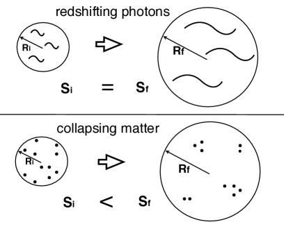
The adiabatic expansion (or contraction) of a gas in equilibrium is reversible. Thus the expansion of the universe by itself is not responsible for any entropy increase in the photons (Fig. A.6 top panel). Another way to understand that the entropy of the photons in the universe remains constant as the universe expands, is to realize that entropy is proportional to the number of photons (Eq. A.27). The number of photons in the volume remains constant and therefore so does the entropy. Thus, we obtain the result indicated in the top panel of Fig. A.6: .
A.4 Gravity and Entropy
In the big bang model, the early universe was in thermal and chemical equilibrium. In the previous section we showed how the expansion of the universe is not responsible for changing the entropy of the photons in the universe. If the universe were in equilibrium, it should have stayed in equilibrium (top panel of Fig. A.6). Our existence shows that the universe could not have started from equilibrium. The missing ingredient that solves this dilemma is gravity. Matter, evenly distributed throughout the universe, has much potential energy and low entropy. In the standard inflationary scenario describing the earliest moments after the big bang, matter originates (during a short period at the end of inflation called reheating) from the decay of the evenly distributed potential energy of a scalar field. ‘False vacuum’ decays into our true vacuum. Vacuum energy cannot clump. However, once the potential energy of the scalar field is dumped almost uniformly into the universe in the form of relativistic particles, these can cool and clump if they have mass (Fig. A.6, lower panel). Unclumped matter has a lower entropy than clumped matter:
| (A.21) |
By we mean the entropy of the phase space volume of the collapsed material as well as the phase space volume of the material expelled during the clumping, plus the entropy of the heat given off during the collapse and dumped into the environment which allowed the unclumped baryons to clump. That is a lot to include but ignoring the full picture has led to much confusion about the relationship between gravity and entropy.
The gravitational potential energy is enormous. In this inflationary picture the potential energy of the false vacuum is the ultimate source of all energy and the matter/antimatter pairs which annihilate and create a bath of photons. Because of an intrinsic asymmetry (baryon non-conservation), the annihilation is incomplete and leaves one baryon for every billion photons. The subsequent cooling (due to the expansion) and clumping of the residual baryons (due to gravity) is the source of all the free energy, dissipative structures and life in the universe (bottom level in Fig. A.1).
The relationship between entropy and gravity is similar to the relationship between energy and heat 200 years ago when the concept of energy conservation in thermodynamics was being developed. It took many decades for the different forms of energy to be recognized. Kinetic energy was different from potential energy, “caloric” became heat energy and Einstein showed us there was energy in mass and in the momentum of massless particles: . It seems to be taking even longer to recognize and define the different forms of entropy, including gravitational entropy and informational entropy (Brissard 2005, Shannon 1950).
There is some confusion about life being in violation of the second law. If how can life be so ordered? The answer is that the order and low entropy of life is maintained by the production and export of entropy. Similarly, there is confusion about clumped material or gravitational structures being in violation of the second law. The resolution is the same: the entropy of the environment needs to be included in the calculation.
Life is trying to maintain its order, while the second law is trying to decrease order. Superficially it seems that life and the second law are at cross purposes. In fact, life and the second law are allies, since the maintainence of a highly ordered structure increases the disorder of the universe more than would be the case without the structure. Similarly, maintaining the low entropy of the structures produced during gravitational collapse (e.g. bipolar outflows of active galactic nuclei and accretion disks) exports entropy such that the net result is an increase of the entropy of the universe, not a decrease.
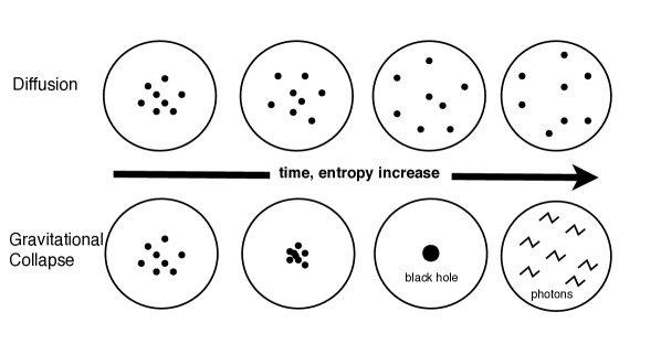
A.4.1 Diffusion and Gravitational Collapse
A misleading idea is that entropy makes things spread out while gravitational collapse makes things clump together, and therefore gravity seems to work against or even violate the second law.
“A recurring theme throughout the life of the universe is the continual struggle between the force of gravity and the tendency for physical systems to evolve toward more disorganized conditions. The amount of disorder in a physical system is measured by its entropy content. In the broadest sense, gravity tends to pull things together and thereby organizes physical structures. Entropy production works in the opposite direction and acts to make physical systems more disorganized and spread out. The interplay between these two competing tendencies provides much of the drama in astrophysics.” Adams and Laughlin (1999).
The part of this quote that is easily misleading is “In the broadest sense, gravity tends to pull things together and thereby organizes physical structures. Entropy production works in the opposite direction …”
See Fig 27.10 of Penrose (2004) for some clarity on this issue. Gravity organizes physical structures but at the expense of disorganizing and expelling other material. This supposed struggle between entropy and gravity is misleading because lots of material is expelled (then ignored in the computation). The heat is ignored too. Consideration of only the centralized accreted remains, does not encompass the full entropic effects of gravitational collapse (Binney and Tremaine 1987).
“If one part of the system becomes well ordered and loses entropy, the system as a whole must pay for it by increasing its entropy somewhere else for compensation” (Adams & Laughlin 1999).
Gravity can only pull things together if angular momentum and energy are exported. If we ignore the entropy associated with the angular momentum and energy export, it is easy to imagine that gravity pulling things together is acting in the opposite direction of the second law, just as it is easy to believe that life is acting in the opposite direction of the second law. If one focuses on the collapsed object while ignoring the increased entropy of the surrounding distribution of stars (which puffs up when part of it collapses), one could believe that:
“The gravitational contribution to entropy is negative and the correlations of clustering decrease this entropy. If we retain the notion that systems evolve in the direction of an entropy extreme (a maximum negative value in the gravitational case), then we should expect infinite systems of galaxies to form tighter and tighter clumps over larger and larger scales…. Spherical systems of stars evolve toward maximum negative gravitational entropy.” (Saslaw 1985 p. 65)
When we ignore the entropy produced during the gravitational collapse of the “spherical systems of stars”, and concentrate only on the collapsed system itself, then Saslaw may be correct, but this seems to contradict the idea that the entropy of a black hole is large and positive . The transition from a negative value to a positive value when an object collapses into its event horizon is problematic (Frampton 2008, Hsu & Reeb 2008).
Neither gravitational collapse nor life violate the second law when we include the increased entropy of the environment. Thus, the maintenance of a fridge or an accretion disk or life, increases the total entropy of the universe.
Thermal (random kinetic energy) can be written as , while gravitational binding energy is . When things are hot, and diffusion dominates. The maximum entropy state is reached when the atoms, or molecules or stars or galaxies fill up the space randomly. They occupy a larger volume of phase space. This is labeled “Diffusion” in the top panel of Fig. A.7. When things are cold, , gravitational collapse occurs and leads to a black hole. Fig. A.7 describes what happens in a universe that is not expanding. However, consider what happens to and when the universe expands (the scale factor increases as is shown in Fig. A.6). Since and any distance scales as we have and . Thus, as the universe expands, decreases faster than and we will always eventually have , which leads to gravitational collapse, black holes and then their evaporation into a diffuse gas of photons – the maximum entropy state of the universe, within which no life can exist. Thus, to depict our universe, the bottom panel of Fig. A.7 should be moved to the right and tacked onto the top panel.
A.4.2 Black Holes and Heat Death
Bekenstein (1973) and Hawking (1974) showed that a black hole of mass has a temperature, and evaporates predominantly as photons when its temperature is hotter than the background temperature. Thus, although the entropy of a black hole, , is sometimes referred to as a maximum entropy state, the sharp gravitational gradient at the event horizon leads to evaporation, photon emission and a higher entropy state of randomly distributed photons. If the background temperature is larger than then the black hole will increase in mass and cool down. However in an expanding universe, and as the universe expands, increases, decreases and eventually we have , which leads to the evaporation of the black hole and the diffusion of the photons produced.
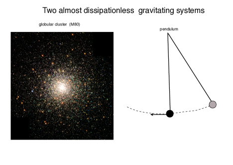
The second law establishes the arrow of time. Since we are far from equilibrium dissipative structures, we must move through time in the direction in which entropy increases and in which free energy is available. Since all observers are dissipative, our existence depends on . The situation is unobservable. This may be an anthropic explanation for the initial low entropy of the universe. No other explanations are known to us. Just as a universe, with a value of a cosmological constant that is too big, is unobservable because stars never form (e.g. Weinberg 1987), so too, a universe that starts at maximum entropy is unobservable. Since life (and any other dissipative structures) needs gradients to form and survive, the initial condition of any universe that contains life will be one of low entropy, not high entropy. You can not start an observable universe from a heat death.
In the multiverse scenario, we imagine universes with varying degrees of baryon non-conservation. If baryon number were conserved, the early universe would have had the same amount of matter as anti-matter. The universe would be filled with a diffuse gas of photons at maximum entropy. There would be no matter homogeneously distributed that would provide the low initial gravitational entropy. Low energy photons, spread out evenly over the volume of the universe, is a maximum entropy state. Baryons spread out evenly, is a minimal gravitational entropy state.
In addition to baryon non-conservation, a requirement for life is that the baryons not be already clumped into black holes. They can be very smoothly distributed, or clumped a bit, but not too much. In other words, non-clumped (but clumpable) matter is required to start the universe at low entropy.
Penrose (1979, 1987, 1989, 2004) has been concerned with the relationship between entropy and gravity for more than three decades (see also Barrow & Tipler 1986). He has stressed the amazingly unlikely initial low gravitational entropy of the universe that ensured that dissipative structures formed as gravity clumped matter and produced gradients to drive dissipative structures.
This low initial entropy of the universe is quantified by the low amplitude of the power spectrum of density perturbations measurable in the cosmic microwave background and in the large scale structure of galaxies. According to the inflationary scenario, these low amplitude density fluctuations have their origin in irreducible vacuum fluctuations that became real during inflation, in a manner analogous to the way electrons and positrons are created out of the vacuum by ultra-strong electric fields between capacitor plates. The initial low amplitude of fluctuations is measured as the amplitude of CMB fluctuations or the amplitude of the power spectrum of large scale structure. The lower the initial values of or , the lower the degree of clumpiness and the lower the initial gravitational entropy of the universe. Penrose (1979) describes these low entropy initial conditions in terms of small values for the Weyl curvature tensor. We are uncertain how to explain the low values of Q or A or the Weyl curvature. In a multiverse scenario, perhaps there is some mother distribution of values from which each universe gets its own initial entropy and ours is low because it has to be for us to evolve and observe it (Tegmark & Rees 1998).
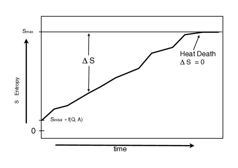
A.5 The Entropy Gap and the Heat Death of the Universe
Is the entropy of the universe getting closer or further from its maximum value ? That is: Is the entropy gap, , increasing or decreasing? Through gravitational collapse, and the irreversible, dissipative processes produced by the density and chemical gradients that result, the entropy of the universe increases, while may be constant (Egan & Lineweaver 2009). Fig. A.9 shows a monotonically decreasing entropy gap leading to a heat death with no possibility for life thereafter. The concept of a heat death was introduced by Thomson (1851, 1862) and has dominated the discussion of the far future fate of the universe.
Tolman (1934) showed that if the universe could bounce back from a contraction into an expansion, a cyclic universe could not be one that is infinitely old, since with each cycle, the entropy of the material would increase, and the cycles would get longer and longer. Steinhardt and Turok (2007) have a model which gets around this entropy problem by reducing entropy with the free energy of a semi-infinite gravitational potential.
In a universe where the energy is conserved (), the free energy available to do work (to maintain far from equilibrium structures) is and this is plotted in Fig. A.10.
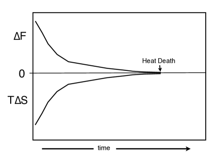
Entropy is the unifying concept of life because the second law is universal; it applies to everything (Schneider & Kay 1994). Man, machine, microbe or the entire cosmos – there is no scale or material to which the second law does not apply. However, the degree to which the equations of thermodynamics apply to near equilibrium situations, steady state situations and far from equilibrium situations is still problematic (see however, Dewar 2003, 2005).
If Darwin had read Carnot (1824), Prigogine (1978) and Penrose (1979, 2004) rather than Newton, Malthus and Lyell, the last paragraph of the Origin of Species would have read something like
“There is grandeur in this view of life, with its dissipative powers, having been originally induced into many forms of far from equilibrium dissipative systems, and that, whilst irreversible processes on this planet have produced entropy according to the fixed second law of thermodynamics, from so simple a low gravitational entropic state, endless forms most beautiful and most wonderful have been and continue to increase the entropy of the universe as they destroy the gradients which spawned them.”
Appendix A. Entropy of Blackbody Photons
Here we show that the entropy of a system of N particles is . For reference, Boltzmann’s constant is . The Stephn-Boltzmann constant . Consider a photon gas at temperature in a volume (e.g. Sears & Salinger 1975). The internal energy is,
| (A.22) |
The entropy is
| (A.23) |
The pressure is
| (A.24) |
and the number of photons is
| (A.26) |
Thus,
| (A.27) |
and to measure the entropy of the microwave background we just need to count photons. If the number of photons in a given volume of the universe is N, then the entropy of photons in that volume is . The photonic entropy of the universe is in the cosmic microwave background. Starlight cannot change that. If all the matter in the universe were transformed into 3 K blackbody radiation, the number of photons would add up to only 1 % of the number of CMB photons. The entropy of the universe would increase by only (Frautschi 1982).
Appendix B. Which Free Energy is most useful F or G?
Thermodynamic equilibrium may be characterized by the minimization of the Helmholtz free energy (Eq. A.1) (e.g. Prigogine 1978). When , no free energy can be extracted from the system, but this is not the same as equilibrium. When there are pressure gradients that can do work and drive organization, i.e., hurricanes, is the most relevant free energy. When pressure cannot be used, i.e., life on Earth, or photon pressure of the cosmic microwave background, then is more relevant.
Chemists are used to dealing with the Gibb’s Free energy of a reaction , where and G is the extractable energy, or free energy under constant pressure conditions (the usual conditions under our stable atmosphere and in the universe except at shock fronts and hurricanes). does not include the work that could be done by a pressure gradient of the atmosphere, while does. We use the Helmholtz free energy because we are interested in the most generic situations. We want to know the extractable energy under any conditions.
Since the free energy can never be more than the internal energy, will always be positive, or . Using Eqs. Eq. A.1, A.22, A.23, the free energy of a photon gas is,
| (A.29) |
This is the work that the photon gas could do if it were surrounded by zero pressure. However the photon gas fills the universe, and can do no work on itself.
The Gibbs free energy of a photon gas in equilibrium does not include work and is equal to zero:
| (A.31) |
No work is used to drive the chemistry-based metabolisms of terrestrial life forms, however some dissipative structures are driven by work and so here we use in our computations. We interpret Eq. A.31 as “no Gibbs free energy can be extracted from a photon gas at equilibrium”
References
- Abe et al. (2008) Abe, S. et al.: 2008, Phys. Rev. Lett. 100, 221803
- Adams and Laughlin (1997) Adams, F. C. and Laughlin, G.: 1997, Reviews of Modern Physics 69, 337
- Adamson et al. (2008) Adamson, P. et al.: 2008, Phys. Rev. Lett. 101, 131802
- Aguirre et al. (2007) Aguirre, A., Gratton, S., and Johnson, M. C.: 2007, Phys. Rev. D 75(12), 123501
- Aguirre and Tegmark (2005) Aguirre, A. and Tegmark, M.: 2005, Journal of Cosmology and Astro-Particle Physics 1, 3
- Ahmed et al. (2004) Ahmed, M., Dodelson, S., Greene, P. B., and Sorkin, R.: 2004, Phys. Rev. D 69(10), 103523
- Albrecht et al. (2006) Albrecht, A., Bernstein, G., Cahn, R., Freedman, W. L., Hewitt, J., Hu, W., Huth, J., Kamionkowski, M., Kolb, E. W., Knox, L., Mather, J. C., Staggs, S., and Suntzeff, N. B.: 2006, ArXiv Astrophysics e-prints
- Allègre et al. (1995) Allègre, C. J., Manhès, G., and Göpel, C.: 1995, Geochim. Cosmochim. Acta 59, 1445
- Allende Prieto (2006) Allende Prieto, C.: 2006, ArXiv Astrophysics e-prints
- Amendola (2000a) Amendola, L.: 2000a, Phys. Rev. D 62(4), 043511
- Amendola (2000b) Amendola, L.: 2000b, MNRAS 312, 521
- Amendola et al. (2007) Amendola, L., Campos, G. C., and Rosenfeld, R.: 2007, Phys. Rev. D 75(8), 083506
- Amendola et al. (2006) Amendola, L., Quartin, M., Tsujikawa, S., and Waga, I.: 2006, Phys. Rev. D 74(2), 023525
- Amendola and Quercellini (2003) Amendola, L. and Quercellini, C.: 2003, Phys. Rev. D 68(2), 023514
- Armendariz-Picon et al. (2000) Armendariz-Picon, C., Mukhanov, V., and Steinhardt, P. J.: 2000, Physical Review Letters 85, 4438
- Armendariz-Picon et al. (2001) Armendariz-Picon, C., Mukhanov, V., and Steinhardt, P. J.: 2001, Phys. Rev. D 63(10), 103510
- Astier et al. (2006) Astier, P., Guy, J., Regnault, N., Pain, R., Aubourg, E., Balam, D., Basa, S., Carlberg, R. G., Fabbro, S., Fouchez, D., Hook, I. M., Howell, D. A., Lafoux, H., Neill, J. D., Palanque-Delabrouille, N., Perrett, K., Pritchet, C. J., Rich, J., Sullivan, M., Taillet, R., Aldering, G., Antilogus, P., Arsenijevic, V., Balland, C., Baumont, S., Bronder, J., Courtois, H., Ellis, R. S., Filiol, M., Gonçalves, A. C., Goobar, A., Guide, D., Hardin, D., Lusset, V., Lidman, C., McMahon, R., Mouchet, M., Mourao, A., Perlmutter, S., Ripoche, P., Tao, C., and Walton, N.: 2006, A&A 447, 31
- Bahcall and Soneira (1980) Bahcall, J. N. and Soneira, R. M.: 1980, ApJS 44, 73
- Balbus and Hawley (2002) Balbus, S. A. and Hawley, J. F.: 2002, ApJ 573, 749
- Barrow (1994) Barrow, J. D.: 1994, The origin of the universe, New York : BasicBooks, c1994.
- Barrow and Tipler (1986) Barrow, J. D. and Tipler, F. J.: 1986, Atmospheric Chemistry & Physics
- Basu and Lynden-Bell (1990) Basu, B. and Lynden-Bell, D.: 1990, QJRAS 31, 359
- Bean et al. (2001) Bean, R., Hansen, S. H., and Melchiorri, A.: 2001, Phys. Rev. D 64(10), 103508
- Bekenstein (1973) Bekenstein, J. D.: 1973, Phys. Rev. D 7, 2333
- Bekenstein (1974) Bekenstein, J. D.: 1974, Phys. Rev. D 9, 3292
- Bekenstein (1981) Bekenstein, J. D.: 1981, Phys. Rev. D 23, 287
- Bekenstein (2005) Bekenstein, J. D.: 2005, Foundations of Physics 35, 1805
- Bell and de Jong (2001) Bell, E. F. and de Jong, R. S.: 2001, ApJ 550, 212
- Bensby and Feltzing (2006) Bensby, T. and Feltzing, S.: 2006, MNRAS 367, 1181
- Bensby et al. (2005) Bensby, T., Feltzing, S., Lundström, I., and Ilyin, I.: 2005, A&A 433, 185
- Bento et al. (2002) Bento, M. C., Bertolami, O., and Sen, A. A.: 2002, Phys. Rev. D 66(4), 043507
- Binney and Tremaine (2008) Binney, J. and Tremaine, S.: 2008, Galactic Dynamics: Second Edition, Princeton University Press
- Bludman (2004) Bludman, S.: 2004, Phys. Rev. D 69(12), 122002
- Bludman and Roos (2001) Bludman, S. A. and Roos, M.: 2001, ApJ 547, 77
- Bostrom (2002) Bostrom, N.: 2002, Anthropic Bias: Observation Selection Effects in Science and Philosophy, Routledge, London
- Bousso (1999) Bousso, R.: 1999, Journal of High Energy Physics 7, 4
- Bousso (2001) Bousso, R.: 2001, Journal of High Energy Physics 4, 35
- Bousso (2002) Bousso, R.: 2002, Reviews of Modern Physics 74, 825
- Bousso et al. (2007) Bousso, R., Harnik, R., Kribs, G. D., and Perez, G.: 2007, Phys. Rev. D 76(4), 043513
- Caldwell (2002) Caldwell, R. R.: 2002, Physics Letters B 545, 23
- Caldwell et al. (1998) Caldwell, R. R., Dave, R., and Steinhardt, P. J.: 1998, Physical Review Letters 80, 1582
- Caldwell et al. (2003) Caldwell, R. R., Kamionkowski, M., and Weinberg, N. N.: 2003, Physical Review Letters 91(7), 071301
- Carroll (2001a) Carroll, S. M.: 2001a, SNAP (SuperNova Acceleration Probe) Yellow Book astro-ph/0107571
- Carroll (2001b) Carroll, S. M.: 2001b, Living Reviews in Relativity 4, 1
- Carroll (2004) Carroll, S. M.: 2004, Spacetime and geometry. An introduction to general relativity, Spacetime and geometry / Sean Carroll. San Francisco, CA, USA: Addison Wesley, ISBN 0-8053-8732-3, 2004, XIV + 513 pp.
- Carter (1974) Carter, B.: 1974, in M. S. Longair (ed.), IAU Symp. 63: Confrontation of Cosmological Theories with Observational Data, pp 291–298
- Carter (1983) Carter, B.: 1983, Philosophical Transactions of the Royal Society A 310, 347
- Chiba et al. (2000) Chiba, T., Okabe, T., and Yamaguchi, M.: 2000, Phys. Rev. D 62(2), 023511
- Chimento et al. (2000) Chimento, L. P., Jakubi, A. S., and Pavón, D.: 2000, Phys. Rev. D 62(6), 063508
- Chimento et al. (2003) Chimento, L. P., Jakubi, A. S., and Pavón, D.: 2003, Phys. Rev. D 67(8), 087302
- Chyba (1999) Chyba, C. F.: 1999, AAS/Division for Planetary Sciences Meeting Abstracts 31, 66.09
- Cleveland et al. (1998) Cleveland, B. T., Daily, T., Davis, R. J., Distel, J. R., Lande, K., Lee, C. K., Wildenhain, P. S., and Ullman, J.: 1998, ApJ 496, 505
- Cohn (1998) Cohn, J. D.: 1998, Ap&SS 259, 213
- Coleman and Roos (2003) Coleman, T. S. and Roos, M.: 2003, Phys. Rev. D 68(2), 027702
- Copeland et al. (2006) Copeland, E. J., Sami, M., and Tsujikawa, S.: 2006, ArXiv e-prints hep-th/0603057
- Courteau and van den Bergh (1999) Courteau, S. and van den Bergh, S.: 1999, AJ 118, 337
- Dalal et al. (2001) Dalal, N., Abazajian, K., Jenkins, E., and Manohar, A. V.: 2001, Physical Review Letters 87(14), 141302
- Davies (1987) Davies, P. C. W.: 1987, Classical and Quantum Gravity 4, L225
- Davies (1994) Davies, P. C. W.: 1994, in J. Halliwell, J. Pérez-Mercader, and W. Zurek (eds.), Physical Origins of Time Asymmetry, pp 119–130
- Davis et al. (2003) Davis, T. M., Davies, P. C. W., and Lineweaver, C. H.: 2003, Classical and Quantum Gravity 20, 2753
- Davis et al. (2007) Davis, T. M., Mörtsell, E., Sollerman, J., Becker, A. C., Blondin, S., Challis, P., Clocchiatti, A., Filippenko, A. V., Foley, R. J., Garnavich, P. M., Jha, S., Krisciunas, K., Kirshner, R. P., Leibundgut, B., Li, W., Matheson, T., Miknaitis, G., Pignata, G., Rest, A., Riess, A. G., Schmidt, B. P., Smith, R. C., Spyromilio, J., Stubbs, C. W., Suntzeff, N. B., Tonry, J. L., Wood-Vasey, W. M., and Zenteno, A.: 2007, ApJ 666, 716
- Dehnen and Binney (1998) Dehnen, W. and Binney, J. J.: 1998, MNRAS 298, 387
- del Campo et al. (2006) del Campo, S., Herrera, R., Olivares, G., and Pavón, D.: 2006, Phys. Rev. D 74(2), 023501
- del Campo et al. (2005) del Campo, S., Herrera, R., and Pavón, D.: 2005, Phys. Rev. D 71(12), 123529
- di Pietro and Claeskens (2003) di Pietro, E. and Claeskens, J.-F.: 2003, MNRAS 341, 1299
- Dicke (1961) Dicke, R. H.: 1961, Nature 192, 440
- Dirac (1937) Dirac, P. A. M.: 1937, Nature 139, 323
- Dirac (1938) Dirac, P. A. M.: 1938, Royal Society of London Proceedings Series A 165, 199
- Dodelson et al. (2000) Dodelson, S., Kaplinghat, M., and Stewart, E.: 2000, Physical Review Letters 85, 5276
- Driver et al. (1994) Driver, S. P., Phillipps, S., Davies, J. I., Morgan, I., and Disney, M. J.: 1994, MNRAS 268, 393
- Durrer and Maartens (2007) Durrer, R. and Maartens, R.: 2007, ArXiv e-prints 0711.0077
- Eddington (1931) Eddington, A. S.: 1931, Nature 127, 447
- Efron (1979) Efron, B.: 1979, Ann. Statist. 7(1)
- Efstathiou (1995) Efstathiou, G.: 1995, MNRAS 274, L73
- Efstathiou and Bond (1999) Efstathiou, G. and Bond, J. R.: 1999, MNRAS 304, 75
- Egan and Lineweaver (2008) Egan, C. A. and Lineweaver, C. H.: 2008, Phys. Rev. D 78(8), 083528
- Egan and Lineweaver (2010a) Egan, C. A. and Lineweaver, C. H.: 2010a, ApJ 710, 1825
- Egan and Lineweaver (2010b) Egan, C. A. and Lineweaver, C. H.: 2010b, How High Could the Entropy be and will the Universe end in a Heat Death?, in preparation
- Eisenhauer et al. (2005) Eisenhauer, F., Genzel, R., Alexander, T., Abuter, R., Paumard, T., Ott, T., Gilbert, A., Gillessen, S., Horrobin, M., Trippe, S., Bonnet, H., Dumas, C., Hubin, N., Kaufer, A., Kissler-Patig, M., Monnet, G., Ströbele, S., Szeifert, T., Eckart, A., Schödel, R., and Zucker, S.: 2005, ApJ 628, 246
- Eisenstein and Hu (1998) Eisenstein, D. J. and Hu, W.: 1998, ApJ 496, 605
- Eisenstein et al. (2005) Eisenstein, D. J., Zehavi, I., Hogg, D. W., Scoccimarro, R., Blanton, M. R., Nichol, R. C., Scranton, R., Seo, H.-J., Tegmark, M., Zheng, Z., Anderson, S. F., Annis, J., Bahcall, N., Brinkmann, J., Burles, S., Castander, F. J., Connolly, A., Csabai, I., Doi, M., Fukugita, M., Frieman, J. A., Glazebrook, K., Gunn, J. E., Hendry, J. S., Hennessy, G., Ivezić, Z., Kent, S., Knapp, G. R., Lin, H., Loh, Y.-S., Lupton, R. H., Margon, B., McKay, T. A., Meiksin, A., Munn, J. A., Pope, A., Richmond, M. W., Schlegel, D., Schneider, D. P., Shimasaku, K., Stoughton, C., Strauss, M. A., SubbaRao, M., Szalay, A. S., Szapudi, I., Tucker, D. L., Yanny, B., and York, D. G.: 2005, ApJ 633, 560
- Eke et al. (2004) Eke, V. R., Frenk, C. S., Baugh, C. M., Cole, S., Norberg, P., Peacock, J. A., Baldry, I. K., Bland-Hawthorn, J., Bridges, T., Cannon, R., Colless, M., Collins, C., Couch, W., Dalton, G., de Propris, R., Driver, S. P., Efstathiou, G., Ellis, R. S., Glazebrook, K., Jackson, C. A., Lahav, O., Lewis, I., Lumsden, S., Maddox, S. J., Madgwick, D., Peterson, B. A., Sutherland, W., and Taylor, K.: 2004, MNRAS 355, 769
- Elgarøy and Multamäki (2007) Elgarøy, O. and Multamäki, T.: 2007, A&A 471, 65
- Elmegreen (2007) Elmegreen, B. G.: 2007, in Y. W. Kang, H.-W. Lee, K.-C. Leung, and K.-S. Cheng (eds.), The Seventh Pacific Rim Conference on Stellar Astrophysics, Vol. 362 of Astronomical Society of the Pacific Conference Series, pp 269–+
- Feng et al. (2006) Feng, B., Li, M., Piao, Y.-S., and Zhang, X.: 2006, Physics Letters B 634, 101
- Ferreira and Joyce (1998) Ferreira, P. G. and Joyce, M.: 1998, Phys. Rev. D 58(2), 023503
- Frampton et al. (2008) Frampton, P., Hsu, S. D. H., Kephart, T. W., and Reeb, D.: 2008, ArXiv e-prints 0801.1847
- Frampton (2009a) Frampton, P. H.: 2009a, ArXiv e-prints 0904.2934
- Frampton (2009b) Frampton, P. H.: 2009b, Journal of Cosmology and Astro-Particle Physics 10, 16
- Frampton and Kephart (2008) Frampton, P. H. and Kephart, T. W.: 2008, Journal of Cosmology and Astro-Particle Physics 6, 8
- França (2006) França, U.: 2006, Physics Letters B 641, 351
- França and Rosenfeld (2004) França, U. and Rosenfeld, R.: 2004, Phys. Rev. D 69(6), 063517
- Frautschi (1982) Frautschi, S.: 1982, Science 217, 593
- Frautschi (1988) Frautschi, S.: 1988, in D. J. Depew, B. H. Weber, and J. D. Smith (eds.), Entropy, information, and evolution : new perspectives on physical and biological evolution, MIT Press, Cambridge, Mass., California State University, Fullerton.
- Fryer and Kalogera (2001) Fryer, C. L. and Kalogera, V.: 2001, ApJ 554, 548
- Fukugita and Peebles (2004) Fukugita, M. and Peebles, P. J. E.: 2004, ApJ 616, 643
- Garriga et al. (1999) Garriga, J., Livio, M., and Vilenkin, A.: 1999, Phys. Rev. D 61(2), 023503
- Garriga and Vilenkin (2000) Garriga, J. and Vilenkin, A.: 2000, Phys. Rev. D 61(8), 083502
- Garriga and Vilenkin (2001) Garriga, J. and Vilenkin, A.: 2001, Phys. Rev. D 64(2), 023517
- Gibbons and Hawking (1977) Gibbons, G. W. and Hawking, S. W.: 1977, Phys. Rev. D 15, 2738
- Glazebrook et al. (2007) Glazebrook, K., Blake, C., Couch, W., Forbes, D., Drinkwater, M., Jurek, R., Pimbblet, K., Madore, B., Martin, C., Small, T., Forster, K., Colless, M., Sharp, R., Croom, S., Woods, D., Pracy, M., Gilbank, D., Yee, H., and Gladders, M.: 2007, ArXiv Astrophysics e-prints
- Gnedin and Gnedin (1998) Gnedin, N. Y. and Gnedin, O. Y.: 1998, ApJ 509, 11
- Gonzalez (1999a) Gonzalez, G.: 1999a, MNRAS 308, 447
- Gonzalez (1999b) Gonzalez, G.: 1999b, Astronomy and Geophysics 40, 25
- Gonzalez et al. (2001) Gonzalez, G., Brownlee, D., and Ward, P.: 2001, Icarus 152, 185
- Gould et al. (1996) Gould, A., Bahcall, J. N., and Flynn, C.: 1996, ApJ 465, 759
- Graham et al. (2007) Graham, A. W., Driver, S. P., Allen, P. D., and Liske, J.: 2007, MNRAS 378, 198
- Grether and Lineweaver (2006) Grether, D. and Lineweaver, C. H.: 2006, ApJ 640, 1051
- Grether and Lineweaver (2007) Grether, D. and Lineweaver, C. H.: 2007, ApJ 669, 1220
- Gunn and Gott (1972) Gunn, J. E. and Gott, J. R. I.: 1972, ApJ 176, 1
- Guo and Zhang (2005) Guo, Z.-K. and Zhang, Y.-Z.: 2005, Phys. Rev. D 71(2), 023501
- Gustafsson (1998) Gustafsson, B.: 1998, Space Science Reviews 85, 419
- Gustafsson et al. (1999) Gustafsson, B., Karlsson, T., Olsson, E., Edvardsson, B., and Ryde, N.: 1999, A&A 342, 426
- Guth (1981) Guth, A. H.: 1981, Phys. Rev. D 23, 347
- Hansen et al. (2004) Hansen, B. M. S., Richer, H. B., Fahlman, G. G., Stetson, P. B., Brewer, J., Currie, T., Gibson, B. K., Ibata, R., Rich, R. M., and Shara, M. M.: 2004, ApJS 155, 551
- Harrison (1995) Harrison, E. R.: 1995, ApJ 446, 63
- Hawking (1976) Hawking, S. W.: 1976, Phys. Rev. D 13, 191
- Hebecker and Wetterich (2001) Hebecker, A. and Wetterich, C.: 2001, Physics Letters B 497, 281
- Heger et al. (2005) Heger, A., Woosley, S. E., and Baraffe, I.: 2005, in R. Humphreys and K. Stanek (eds.), The Fate of the Most Massive Stars, Vol. 332 of Astronomical Society of the Pacific Conference Series, pp 339–+
- Henry (2006) Henry, T. J.: 2006, RECONS database
-
Hinshaw (2006)
Hinshaw, G.: 2006,
Legacy Archive for Microwave Background Data Analaysis
(LAMBDA),
Online Archive: http://lambda.gsfc.nasa.gov/product/map/
current/params/lcdm_wmap_sdss.cfm - Hopkins (2006) Hopkins, A. M.: 2006, ArXiv e-prints astro.ph/0611283
- Hulse and Taylor (1975) Hulse, R. A. and Taylor, J. H.: 1975, ApJ 195, L51
- Huterer and Cooray (2005) Huterer, D. and Cooray, A.: 2005, Phys. Rev. D 71(2), 023506
- Ida and Lin (2005) Ida, S. and Lin, D. N. C.: 2005, ApJ 626, 1045
- Jarrett et al. (2003) Jarrett, T. H., Chester, T., Cutri, R., Schneider, S. E., and Huchra, J. P.: 2003, AJ 125, 525
- Jaynes (1968) Jaynes, E. T.: 1968, IEEE Transactions on System Science and Cybernetics SSC-4, 227
- Jordan (1955) Jordan, P.: 1955, Schwerkraft und Weltall, Braunschweig, Germany
- Kamenshchik et al. (2001) Kamenshchik, A., Moschella, U., and Pasquier, V.: 2001, Physics Letters B 511, 265
- Kolb and Turner (1981) Kolb, E. W. and Turner, M. S.: 1981, Nature 294, 521
- Kolb and Turner (1990) Kolb, E. W. and Turner, M. S.: 1990, The early universe, Frontiers in Physics, Reading, MA: Addison-Wesley, 1988, 1990
- Kroupa (2002) Kroupa, P.: 2002, Science 295, 82
- Kuchner and Seager (2005) Kuchner, M. J. and Seager, S.: 2005, ArXiv e-prints astro-ph/0504214
- Lanzetta et al. (2002) Lanzetta, K. M., Yahata, N., Pascarelle, S., Chen, H.-W., and Fernández-Soto, A.: 2002, ApJ 570, 492
- Layzer (2009) Layzer, D.: 2009, www.informationphilosopher.com
- Linde (1982) Linde, A. D.: 1982, Physics Letters B 108, 389
- Linde (2009) Linde, A. D.: 2009, private communication
- Linder (1997) Linder, E.: 1997, First Principles of Cosmology, First Principles of Cosmology, by E.V. Linder. Addison-Wesley, Harlow, England, 1997
- Linder (2006a) Linder, E. V.: 2006a, Astroparticle Physics 26, 102
- Linder (2006b) Linder, E. V.: 2006b, Phys. Rev. D 73(6), 063010
- Linder and Huterer (2005) Linder, E. V. and Huterer, D.: 2005, Phys. Rev. D 72(4), 043509
- Lineweaver (1998) Lineweaver, C. H.: 1998, ApJ 505, L69
- Lineweaver (1999) Lineweaver, C. H.: 1999, Science 284, 1503
- Lineweaver (2001) Lineweaver, C. H.: 2001, Icarus 151, 307
- Lineweaver and Davis (2002) Lineweaver, C. H. and Davis, T. M.: 2002, Astrobiology 2, 293
- Lineweaver and Davis (2003) Lineweaver, C. H. and Davis, T. M.: 2003, Astrobiology 3, 241
- Lineweaver and Egan (2007) Lineweaver, C. H. and Egan, C. A.: 2007, ApJ 671, 853
- Lineweaver and Egan (2008) Lineweaver, C. H. and Egan, C. A.: 2008, Physics of Life Reviews 5, 225
- Lineweaver and Grether (2003) Lineweaver, C. H. and Grether, D.: 2003, ApJ 598, 1350
- Loveday (2000) Loveday, J.: 2000, MNRAS 312, 557
- Lynden-Bell (1967) Lynden-Bell, D.: 1967, MNRAS 136, 101
- Malquarti et al. (2003) Malquarti, M., Copeland, E. J., and Liddle, A. R.: 2003, Phys. Rev. D 68(2), 023512
- Martel et al. (1998) Martel, H., Shapiro, P. R., and Weinberg, S.: 1998, ApJ 492, 29
- Mather et al. (1994) Mather, J. C., Cheng, E. S., Cottingham, D. A., Eplee, Jr., R. E., Fixsen, D. J., Hewagama, T., Isaacman, R. B., Jensen, K. A., Meyer, S. S., Noerdlinger, P. D., Read, S. M., Rosen, L. P., Shafer, R. A., Wright, E. L., Bennett, C. L., Boggess, N. W., Hauser, M. G., Kelsall, T., Moseley, Jr., S. H., Silverberg, R. F., Smoot, G. F., Weiss, R., and Wilkinson, D. T.: 1994, ApJ 420, 439
- Mather et al. (1999) Mather, J. C., Fixsen, D. J., Shafer, R. A., Mosier, C., and Wilkinson, D. T.: 1999, ApJ 512, 511
- Mbonye (2004) Mbonye, M. R.: 2004, Modern Physics Letters A 19, 117
- Mersini-Houghton and Adams (2008) Mersini-Houghton, L. and Adams, F. C.: 2008, Classical and Quantum Gravity 25(16), 165002
- Metropolis and Ulam (1949) Metropolis, N. and Ulam, S.: 1949, Journal of the American Statistical Association 44(247), 335
- Nagamine et al. (2006) Nagamine, K., Ostriker, J. P., Fukugita, M., and Cen, R.: 2006, ApJ 653, 881
- Nojiri and Odintsov (2006) Nojiri, S. and Odintsov, S. D.: 2006, Physics Letters B 637, 139
- Nordström et al. (2004) Nordström, B., Mayor, M., Andersen, J., Holmberg, J., Pont, F., Jørgensen, B. R., Olsen, E. H., Udry, S., and Mowlavi, N.: 2004, A&A 418, 989
- Olivares et al. (2005) Olivares, G., Atrio-Barandela, F., and Pavón, D.: 2005, Phys. Rev. D 71(6), 063523
- Olivares et al. (2007) Olivares, G., Atrio-Barandela, F., and Pavon, D.: 2007, ArXiv e-prints 0706.3860 706
- Özer and Taha (1987) Özer, M. and Taha, M. O.: 1987, Nuclear Physics B 287, 776
- Page (1981) Page, D. N.: 1981, General Relativity and Gravitation 13, 1117
- Page and McKee (1981) Page, D. N. and McKee, M. R.: 1981, Nature 291, 44
- Pagel (1997) Pagel, B. E. J.: 1997, Nucleosynthesis and Chemical Evolution of Galaxies, Nucleosynthesis and Chemical Evolution of Galaxies, by Bernard E. J. Pagel, pp. 392. ISBN 0521550610. Cambridge, UK: Cambridge University Press, October 1997.
- Pavón and Zimdahl (2005) Pavón, D. and Zimdahl, W.: 2005, Physics Letters B 628, 206
- Peacock (1999) Peacock, J. A.: 1999, Cosmological Physics, Cosmological Physics, by John A. Peacock, pp. 704. ISBN 052141072X. Cambridge, UK: Cambridge University Press, January 1999.
- Peebles and Vilenkin (1999) Peebles, P. J. E. and Vilenkin, A.: 1999, Phys. Rev. D 59(6), 063505
- Penrose (1979) Penrose, R.: 1979, in S. W. Hawking and W. Israel (eds.), General Relativity: An Einstein centenary survey, pp 581–638
- Penrose (1987) Penrose, R.: 1987, Newton, quantum theory and reality., pp 17–49, Three hundred years of gravitation, p. 17 - 49
- Penrose (2004) Penrose, R.: 2004, The road to reality : a complete guide to the laws of the universe, The road to reality : a complete guide to the laws of the universe, by Roger Penrose. London: Jonathan Cape, 2004
- Perlmutter et al. (1999) Perlmutter, S., Aldering, G., Goldhaber, G., Knop, R. A., Nugent, P., Castro, P. G., Deustua, S., Fabbro, S., Goobar, A., Groom, D. E., Hook, I. M., Kim, A. G., Kim, M. Y., Lee, J. C., Nunes, N. J., Pain, R., Pennypacker, C. R., Quimby, R., Lidman, C., Ellis, R. S., Irwin, M., McMahon, R. G., Ruiz-Lapuente, P., Walton, N., Schaefer, B., Boyle, B. J., Filippenko, A. V., Matheson, T., Fruchter, A. S., Panagia, N., Newberg, H. J. M., Couch, W. J., and The Supernova Cosmology Project: 1999, ApJ 517, 565
- Pogosian and Vilenkin (2007) Pogosian, L. and Vilenkin, A.: 2007, Journal of Cosmology and Astro-Particle Physics 1, 25
- Press and Schechter (1974) Press, W. H. and Schechter, P.: 1974, ApJ 187, 425
- Ratra and Peebles (1988) Ratra, B. and Peebles, P. J. E.: 1988, Phys. Rev. D 37, 3406
- Reddy et al. (2003) Reddy, B. E., Tomkin, J., Lambert, D. L., and Allende Prieto, C.: 2003, MNRAS 340, 304
- Reid (2002) Reid, I. N.: 2002, PASP 114, 306
- Riess et al. (1998) Riess, A. G., Filippenko, A. V., Challis, P., Clocchiatti, A., Diercks, A., Garnavich, P. M., Gilliland, R. L., Hogan, C. J., Jha, S., Kirshner, R. P., Leibundgut, B., Phillips, M. M., Reiss, D., Schmidt, B. P., Schommer, R. A., Smith, R. C., Spyromilio, J., Stubbs, C., Suntzeff, N. B., and Tonry, J.: 1998, AJ 116, 1009
- Riess et al. (2007) Riess, A. G., Strolger, L.-G., Casertano, S., Ferguson, H. C., Mobasher, B., Gold, B., Challis, P. J., Filippenko, A. V., Jha, S., Li, W., Tonry, J., Foley, R., Kirshner, R. P., Dickinson, M., MacDonald, E., Eisenstein, D., Livio, M., Younger, J., Xu, C., Dahlén, T., and Stern, D.: 2007, ApJ 659, 98
- Riess et al. (2004) Riess, A. G., Strolger, L.-G., Tonry, J., Casertano, S., Ferguson, H. C., Mobasher, B., Challis, P., Filippenko, A. V., Jha, S., Li, W., Chornock, R., Kirshner, R. P., Leibundgut, B., Dickinson, M., Livio, M., Giavalisco, M., Steidel, C. C., Benítez, T., and Tsvetanov, Z.: 2004, ApJ 607, 665
- Robles et al. (2008a) Robles, J. A., Egan, C. A., and Lineweaver, C. H.: 2008a, in Australian Space Science Conference Series: 8th Conference Proceedings
- Robles et al. (2008b) Robles, J. A., Lineweaver, C. H., Grether, D., Flynn, C., Egan, C. A., Pracy, M. B., Holmberg, J., and Gardner, E.: 2008b, ApJ 684, 691
- Robles et al. (2008c) Robles, J. A., Lineweaver, C. H., Grether, D., Flynn, C., Egan, C. A., Pracy, M. B., Holmberg, J., and Gardner, E.: 2008c, ApJ 689, 1457
- Rocha-Pinto et al. (2000) Rocha-Pinto, H. J., Scalo, J., Maciel, W. J., and Flynn, C.: 2000, A&A 358, 869
- Sahni (2002) Sahni, V.: 2002, Classical and Quantum Gravity 19, 3435
- Sahni and Wang (2000) Sahni, V. and Wang, L.: 2000, Phys. Rev. D 62(10), 103517
- Sassi and Bonometto (2007) Sassi, G. and Bonometto, S. A.: 2007, New Astronomy 12, 353
- Scherrer (2005) Scherrer, R. J.: 2005, Phys. Rev. D 71(6), 063519
- Seljak et al. (2006) Seljak, U., Slosar, A., and McDonald, P.: 2006, Journal of Cosmology and Astro-Particle Physics 10, 14
- Soderblom (1983) Soderblom, D. R.: 1983, ApJS 53, 1
- Spergel et al. (2007) Spergel, D. N., Bean, R., Doré, O., Nolta, M. R., Bennett, C. L., Dunkley, J., Hinshaw, G., Jarosik, N., Komatsu, E., Page, L., Peiris, H. V., Verde, L., Halpern, M., Hill, R. S., Kogut, A., Limon, M., Meyer, S. S., Odegard, N., Tucker, G. S., Weiland, J. L., Wollack, E., and Wright, E. L.: 2007, ApJS 170, 377
- Spergel et al. (2006) Spergel, D. N., Bean, R., Dore’, O., Nolta, M. R., Bennett, C. L., Hinshaw, G., Jarosik, N., Komatsu, E., Page, L., Peiris, H. V., Verde, L., Barnes, C., Halpern, M., Hill, R. S., Kogut, A., Limon, M., Meyer, S. S., Odegard, N., Tucker, G. S., Weiland, J. L., Wollack, E., and Wright, E. L.: 2006, astro-ph/0603449 http://lambda.gsfc.nasa.gov/product/map/dr2/params/lcdm-all.cfm
- Steinhardt (2008) Steinhardt, P.: 2008, private communication
- Steinhardt (2003) Steinhardt, P. J.: 2003, Royal Society of London Philosophical Transactions Series A 361, 2497
- Steinhardt et al. (1999) Steinhardt, P. J., Wang, L., and Zlatev, I.: 1999, Phys. Rev. D 59(12), 123504
- Strominger and Vafa (1996) Strominger, A. and Vafa, C.: 1996, Physics Letters B 379, 99
- Susskind (1995) Susskind, L.: 1995, Journal of Mathematical Physics 36, 6377
- Szydłowski et al. (2006) Szydłowski, M., Kurek, A., and Krawiec, A.: 2006, Physics Letters B 642, 171
- ’t Hooft (1993) ’t Hooft, G.: 1993, ArXiv General Relativity and Quantum Cosmology e-prints
- Thomas (2009) Thomas, A.: 2009, www.ipod.org.uk
- Thompson et al. (2006) Thompson, R. I., Eisenstein, D., Fan, X., Dickinson, M., Illingworth, G., and Kennicutt, Jr., R. C.: 2006, ApJ 647, 787
- Thomson (1852) Thomson, W.: 1852, Philosophical Magazine 4, 304
- Turner (2001) Turner, M. S.: 2001, Nuclear Physics B Proceedings Supplements 91, 405
- Valenti and Fischer (2005) Valenti, J. A. and Fischer, D. A.: 2005, ApJS 159, 141
- Vilenkin (1995a) Vilenkin, A.: 1995a, Phys. Rev. D 52, 3365
- Vilenkin (1995b) Vilenkin, A.: 1995b, Physical Review Letters 74, 846
- Vilenkin (1996a) Vilenkin, A.: 1996a, in N. Sanchez and A. Zichichi (eds.), String Gravity and Physics at the Planck Energy Scale, pp 345–367
- Vilenkin (1996b) Vilenkin, A.: 1996b, in K. Sato, T. Suginohara, and N. Sugiyama (eds.), Cosmological Constant and the Evolution of the Universe, pp 161–+
- Wang et al. (2000) Wang, L., Caldwell, R. R., Ostriker, J. P., and Steinhardt, P. J.: 2000, ApJ 530, 17
- Wang and Mukherjee (2006) Wang, Y. and Mukherjee, P.: 2006, ApJ 650, 1
- Wang and Tegmark (2004) Wang, Y. and Tegmark, M.: 2004, Physical Review Letters 92(24), 241302
- Wang and Tegmark (2005) Wang, Y. and Tegmark, M.: 2005, Phys. Rev. D 71(10), 103513
- Weinberg (1987) Weinberg, S.: 1987, Physical Review Letters 59, 2607
- Weinberg (1989) Weinberg, S.: 1989, Reviews of Modern Physics 61, 1
- Weinberg (2000a) Weinberg, S.: 2000a, Phys. Rev. D 61(10), 103505
- Weinberg (2000b) Weinberg, S.: 2000b, ArXiv e-prints astro-ph/0005265
- Weisberg and Taylor (2005) Weisberg, J. M. and Taylor, J. H.: 2005, in F. A. Rasio and I. H. Stairs (eds.), Binary Radio Pulsars, Vol. 328 of Astronomical Society of the Pacific Conference Series, pp 25–+
- Wetherill (1996) Wetherill, G. W.: 1996, in L. R. Doyle (ed.), Circumstellar Habitable Zones, p. 193
- Wood-Vasey et al. (2007) Wood-Vasey, W. M., Miknaitis, G., Stubbs, C. W., Jha, S., Riess, A. G., Garnavich, P. M., Kirshner, R. P., Aguilera, C., Becker, A. C., Blackman, J. W., Blondin, S., Challis, P., Clocchiatti, A., Conley, A., Covarrubias, R., Davis, T. M., Filippenko, A. V., Foley, R. J., Garg, A., Hicken, M., Krisciunas, K., Leibundgut, B., Li, W., Matheson, T., Miceli, A., Narayan, G., Pignata, G., Prieto, J. L., Rest, A., Salvo, M. E., Schmidt, B. P., Smith, R. C., Sollerman, J., Spyromilio, J., Tonry, J. L., Suntzeff, N. B., and Zenteno, A.: 2007, ArXiv Astrophysics e-prints
- Wright et al. (2004) Wright, J. T., Marcy, G. W., Butler, R. P., and Vogt, S. S.: 2004, ApJS 152, 261
- Yang and Wang (2005) Yang, G. and Wang, A.: 2005, General Relativity and Gravitation 37, 2201
- Zel’Dovich (1967) Zel’Dovich, Y. B.: 1967, Soviet Journal of Experimental and Theoretical Physics Letters 6, 316
- Zhang (2005) Zhang, X.: 2005, Modern Physics Letters A 20, 2575
- Zimdahl et al. (2001) Zimdahl, W., Pavón, D., and Chimento, L. P.: 2001, Physics Letters B 521, 133
- Zlatev et al. (1999) Zlatev, I., Wang, L., and Steinhardt, P. J.: 1999, Physical Review Letters 82, 896