Stability verification for monotone systems using homotopy algorithms

Abstract

A monotone self-mapping of the nonnegative orthant induces a monotone discrete-time dynamical system which evolves on the same orthant. If with respect to this system the origin is attractive then there must exists points whose image under the monotone map is strictly smaller than the original point, in the component-wise partial ordering. Here it is shown how such points can be found numerically, leading to a recipe to compute order intervals that are contained in the region of attraction and where the monotone map acts essentially as a contraction. An important application is the numerical verification of so-called generalized small-gain conditions that appear in the stability theory of large-scale systems.

1 Introduction

By ${\mathbb{R}_{+}}$ we denote the nonnegative real numbers, $[0,\infty)$. A class $\mathcal{K}$ function is a continuous function $\gamma\colon{\mathbb{R}_{+}}\to{\mathbb{R}_{+}}$ that satisfies $\gamma(0)=0$ and is strictly increasing. The function $\gamma$ is of class $\mathcal{K}_{\infty}\subset\mathcal{K}$ if in addition $\gamma$ is unbounded. Note that with respect to composition the class $\mathcal{K}_{\infty}$ is a group and the class $\mathcal{K}$ a semi-group. Moreover, sums and positive multiples of $\mathcal{K}$ functions are again $\mathcal{K}$ functions.

The nonnegative orthant $\mathbb{R}^{n}_{+}$ induces a partial order on $\mathbb{R}^{n}$, which coincides with the component wise ordering, and we write for $x,y\in\mathbb{R}^{n}$, $x\leq y$ if $y-x\in\mathbb{R}^{n}_{+}$, $x<y$ if [$x\leq y$ and $x\neq y$], and $x\ll y$ if $y-x\in\operatorname{int}\mathbb{R}^{n}_{+}$, the interior of $\mathbb{R}^{n}_{+}$.

A map $T\colon\mathbb{R}^{n}_{+}\to\mathbb{R}^{n}_{+}$ is monotone if $x\leq y$ implies $Tx\leq Ty$. For any $\mathcal{K}_{\infty}$ function $\rho$, the map $D=\operatorname{diag}(\rho)\colon\mathbb{R}^{n}_{+}\to\mathbb{R}^{n}_{+}$ defined by $(Dx)_{i}=\rho(x_{i})$ is an example of a monotone map.

We consider the following problem:

Problem 1

Let a monotone, continuous map $T\colon\mathbb{R}^{n}_{+}\to\mathbb{R}^{n}_{+}$ with $T(0)=0$ and a real number $r>0$ be given. Find $s^{*}\in\mathbb{R}^{n}_{+}$ satisfying

1. $Ts^{*}\ll s^{*}$ (which implies $s^{*}\gg 0$),

2. $\|s^{*}\|_{1}=r$, and

3. $Ts\ngeq s$ for all $s\in[0,s^{*}],s\neq 0$.∎

The existence of such an $s^{*}$ (for sufficiently small $r>0$) is a necessary and sufficient condition for asymptotic stability of the origin with respect to the discrete time system

$$s^{+}=Ts,\quad s\in\mathbb{R}^{n}_{+}.$$ (1)

It also arises as a so-called generalized small-gain condition RufferDashkovskiy:2009:Local-ISS-of-large-scale-interconnection: . If it is satisfied then the set $[0,s^{*}]$ is contained in the region of attraction. Moreover, in this case also the system with input,

$$s^{+}=Ts+w,\quad s,w\in\mathbb{R}^{n}_{+},$$ (2)

is locally input-to-state stable GaoLin:2000:On-equivalent-notions-of-input-to-state-: ; JiangWang:2001:Input-to-state-stability-for-discrete-ti: , and knowledge of $s^{*}$ yields estimates for the sets of admissible inputs and initial conditions which result in bounded outputs, cf. RufferDashkovskiy:2009:Local-ISS-of-large-scale-interconnection: .

The numerical solution of this problem is interesting in two aspects: First of all, it provides a numerical way to make a qualitative assertion. Secondly, this assertion is not only of qualitative nature (i.e., a system is stable in some sense), but also quantitative in that an estimate for the region of attraction is obtained as well.

The numerical solution of this problem is interesting for several applications: In the context of large-scale interconnections of nonlinear systems the solution to Problem 1 can assert (local) input-to-state stability of interconnections of many systems in arbitrary interconnection topology. This in turn can be useful for formation control TannerPappasKumar:2004:Leader-to-formation-stability: or the effective implementation of decentralized model predictive control RaimondoMagniScattolini:2007:Decentralized-MPC-of-nonlinear-systems:-: . Furthermore, in the same context the knowledge of $s^{*}$ can be used to find a locally Lipschitz continuous Lyapunov function for the composite large-scale system. Another application is in queuing theory. Here the solution to Problem 1 can be used to ascertain that a given switching policy stabilizes a flow switching network via the use of a monotone monodromy operator, cf. FeoktistovaMatveev:2009:Dynamic-interactive-stabilization-of-the: , at least for specified range of initial buffer levels and bounded inflow.

It is known that a solution to Problem 1 must exist for any $r>0$ if the origin is globally attractive with respect to (1). In this case necessarily it holds that $Ts\ngeq s$ for all $s\in\mathbb{R}^{n}_{+},s\neq 0$, and by virtue of a topological fixed point result, for every $r>0$, there exists an $s^{*}$ with $\|s^{*}\|_{1}=r$ satisfying $Ts^{*}\ll s^{*}$. However, even if $T\colon\mathbb{R}^{n}_{+}\to\mathbb{R}^{n}_{+}$ is monotone, continuous, and satisfies $T(0)=0$ as well as $Ts\ngeq s$ for all $s\in\mathbb{R}^{n}_{+},s\neq 0$, the origin is not necessarily globally attractive with respect to (1) (but it is so locally). For $T$ of particular form a sufficient condition for global asymptotic stability of the origin with respect to (1) is the existence of a diagonal map $D=\operatorname{diag}(\mbox{id}+\rho)\colon\mathbb{R}^{n}_{+}\to\mathbb{R}^{n}_{+}$ with $\rho\in\mathcal{K}_{\infty}$ such that for all $s\neq 0$, $(D\circ T)s\ngeq s$, or, equivalently $(T\circ D)s\ngeq s$. In this case the system (2) is input-to-state stable Ruffer:2009:Monotone-inequalities-dynamical-systems-: ; Ruffer:2009:Small-gain-conditions-and-the-comparison: .

Also known is that if $T$ satisfies $T(s\oplus v)=Ts\oplus Tv$ for all $s,v\in\mathbb{R}^{n}_{+}$, where $\oplus$ denotes component-wise maximization, then $T$ must be of the form $(Ts)_{i}=\max_{j}\gamma_{ij}(s_{j})$ for all $i,j$, where $\gamma_{ij}\colon{\mathbb{R}_{+}}\to{\mathbb{R}_{+}}$ are nondecreasing functions. In this case $T$ has been termed max-preserving. Here, the condition $Ts\ngeq s$ for all $s\neq 0$ is equivalent to the cycle condition, which assumes that $\gamma_{i_{1}i_{2}}\circ\gamma_{i_{2}i_{3}}\circ\ldots\circ\gamma_{i_{k-1}i_{k}}\circ\gamma_{i_{k}i_{k}}<\mbox{id}$ for all finite ordered sequences $(i_{1},i_{2},\ldots,i_{k})\subset\{1,\ldots,n\}^{k}$. If this condition holds then with $e$ denoting the vector $(1,\ldots,1)^{T}$ and $t>0$ one has for $q(t):=\max\{te,T(te),\ldots,T^{n-1}(te)\}\in\mathbb{R}^{n}_{+}$ a continuous path $q\colon{\mathbb{R}_{+}}\to\mathbb{R}^{n}_{+}$ which is unbounded and nondecreasing in every component and satisfies $T(q(t))\leq q(t)$. Re-parametrization yields a path $\widetilde{q}(r)$ satisfying $\|\widetilde{q}(r)\|_{1}=r$, which can be interpreted as a parametrized “almost” solution to Problem 1, cf. KarafyllisJiang:2009:A-Vector-Small-Gain-Theorem-for-General-: .

In the linear case the action of $T$ can be represented by multiplication with a nonnegative matrix (i.e., every component is nonnegative), which we also denote by $T\in\mathbb{R}_{+}^{n\times n}$. It is known that the following are equivalent:

1. $Ts\ngeq s$ for all $s\in\mathbb{R}^{n}_{+},s>0$;

2. there exists a $D=\operatorname{diag}(\mbox{id}+\rho)$ with $\rho\in\mathcal{K}_{\infty}$ such that $(T\circ D)s\ngeq s$ for all $s\in\mathbb{R}^{n}_{+},s>0$ (equivalently, $(D\circ T)s\ngeq s$ for all $s\in\mathbb{R}^{n}_{+},s>0$);

3. the spectral radius of $T$ is less than one;

4. there exists a unit vector $s^{*}\gg 0$ (with respect to the 1-norm) such that $Ts^{*}\ll s^{*}$, hence also the ray given by $rs^{*}$, $r\in{\mathbb{R}_{+}}$ satisfies $T(rs^{*})\ll rs^{*}$ for $r>0$ and $\|rs^{*}\|_{1}=r$;

5. the inverse of $I-T$ exists and is given by the nonnegative matrix $\sum_{k\geq 0}T^{k}$.

The existence of the vector $s^{*}$ is of course related to the classical Perron-Frobenius theory. If $T$ is primitive then $s^{*}$ is just the positive Perron-Frobenius root corresponding to the maximal eigenvalue, which coincides with the spectral radius. Further extensions of the classical Perron-Frobenius theory exist for special classes of nonlinear maps, in particular for homogeneous maps and for concave maps, cf. AeyelsDe-Leenheer:2002:Extension-of-the-Perron-Frobenius-theore: ; Krause:2001:Concave-Perron-Frobenius-theory-and-appl: .

In this paper we propose the use of a homotopy method to find a point $s^{*}$ satisfying $Ts^{*}\ll s^{*}$, $\|s^{*}\|_{1}$ for any given $r>0$. Our method of choice is the K1 algorithm proposed by Eaves Eaves:1972:Homotopies-for-computation-of-fixed-poin: as a computational version of a topological fixed point theorem. There are, however, more elaborate choices of related algorithms available as well, cf. AllgowerGeorg:1980:Simplicial-and-continuation-methods-for-: ; AllgowerGeorg:1990:Numerical-continuation-methods: for an overview. While these algorithm have the potential of admitting faster convergence, they tend to be more complicated to implement. One particular advantage of homotopy methods is that they offer global convergence: If there exists a point $s^{*}$ with $\|s^{*}\|_{1}=r$ with the desired properties then it will be found. This has to bee seen in contrast to methods based on Newton steps, which only guarantee convergence if the algorithm is started sufficiently close to $s^{*}$. Moreover, Newton methods usually assume some level of smoothness, whereas homotopy methods only require continuity.

Once the point $s^{*}$ has been computed, the remaining verification of property 3 in Problem 1 is an easy task: It only needs to be checked that the sequence $T^{k}(s^{*})$ converges to zero. It is then a consequence of monotonicity that property 3 must hold.

The paper is organized as follows. In Section 2 a few facts about monotone self-mappings of the nonnegative orthant and their induced discrete-time systems are recalled. In particular, the topological fixed point theorem by Knaster, Kuratowski, and Mazurkiewicz is discussed. A brief and informal description of some of the underlying principles of Eaves’ and other homotopy algorithms is given in Section 3. A MATLAB version of Eaves’ K1 algorithm is provided in Section 4. Section 5 explains a short procedure to solve Problem 1 based on the use of a homotopy algorithm and the computation of one trajectory of system (1). This is followed by several numerical examples in Section 6.

2 Monotone maps and monotone discrete-time systems

This section collects a few theoretical results from the literature.

Throughout this section let $T\colon\mathbb{R}^{n}_{+}\to\mathbb{R}^{n}_{+}$ be monotone and continuous with $T(0)=0$. Consider also the induced discrete-time systems (1) and (2). Denote their respective solutions for initial condition $s^{0}\in\mathbb{R}^{n}_{+}$ and, in case of (2), input sequence $w=\{w(k)\in\mathbb{R}^{n}_{+}\colon k\geq 0\}$, at time $k\geq 0$ by $\phi_{\eqref{eq:8}}(k,s^{0})$ and $\phi_{\eqref{eq:9}}(k,s^{0},w)$, respectively. If the reference to a particular system is clear from the context we omit the reference to the system. Observe that both systems satisfy the ordering of solutions principle: If $s^{0}\leq v^{0}$ and for all $k\geq 0$, $w(k)\leq u(k)$ (which we abbreviate by $w\leq u$), then also $\phi_{\eqref{eq:8}}(k,s^{0})\leq\phi_{\eqref{eq:8}}(k,v^{0})$ and $\phi_{\eqref{eq:9}}(k,s^{0},w)\leq\phi_{\eqref{eq:9}}(k,v^{0},u)$ for all $k\geq 0$.

We denote the sphere in $\mathbb{R}^{n}_{+}$ of radius $r>0$ with respect to the 1-norm by $S_{r}=\{s\in\mathbb{R}^{n}_{+}\colon\|s\|_{1}=\sum_{i}s_{i}=r\}$. Observe that $S_{r}$ is an $(n-1)$ simplex.

Theorem 2.1

Let $T\colon\mathbb{R}^{n}_{+}\to\mathbb{R}^{n}_{+}$ be monotone and continuous with $T(0)=0$. Assume that the origin is attractive with respect to (1) and denote the domain of attraction by $\mathcal{B}$. Then the following assertions holds:

1. For every $s\in\mathcal{B}$, $s\neq 0$, necessarily $Ts\ngeq s$.

2. If $R\in\mathbb{R}$, $R>0$ is such that $S_{R}\subset\mathcal{B}$ then for all $r\in(0,R]$ there exists a point $s\in S_{r}$, $s\gg 0$, satisfying $Ts\ll s$.

3. The origin is stable in the sense of Lyapunov, i.e., for every $\varepsilon>0$ there exists a $\delta>0$ such that $\|s\|_{1}<\delta$ implies $\|Ts\|_{1}<\varepsilon$.

A proof can be found in Ruffer:2009:Monotone-inequalities-dynamical-systems-: . The first assertion is not difficult to prove directly, and the third follows from the second. The second assertion is the most technical, and it is based on the covering theorem by Knaster, Kuratowski, and Mazurkiewicz (KKM) KnasterKuratowskiMazurkiewicz:1929:Ein-Beweis-des-Fixpunktsatzes-fur-n-dime: . Our reasoning is based on the extension given in Lassonde:1990:Sur-le-principe-KKM: which allows to consider coverings of open instead of closed sets. The argument is basically the following: One has $Ts\ngeq s$ for all $s\in\ S_{r}$, and $S_{r}$ is a simplex. This ordering condition implies that the simplex is covered by the sets

$$\Omega_{i}=\{s\in S_{r}\colon(Ts)_{i}<s_{i}\}.$$

Moreover, no $\Omega_{i}$ can contain the face $\sigma_{i}\subset S_{r}$ opposite of the vertex $re_{i}\in\Omega_{i}$, where $e_{i}$ denotes the $i$th unit vector. On the other hand, every $k$-dimensional simplex $\sigma=\operatorname{co}\{re_{i}\}_{i\in\{i_{1},\ldots,i_{k}\}}$, $k\leq n-1$, is contained in the union $\bigcup_{i\in\{i_{1},\ldots,i_{k}\}}\Omega_{i}$. These are the prerequisites of the KKM Theorem, which then ascertains that the intersection $\bigcap\Omega_{i}$ must be nonempty. The proof of the KKM Theorem is based on the fact that every simplicial refinement of $S_{r}$ must contain at least one special simplex, which is again covered by all sets $\Omega_{i}$ but not by any strict subclass of $\{\Omega_{1},\ldots,\Omega_{n}\}$. As the size of the refinements tends to zero, this special simplex contracts to a point — the point of interest $s^{*}\in S_{r}$ satisfying $Ts^{*}\ll s^{*}$. In essence this proof technique relies on a fine discretization of $S_{r}$ and an exhaustive search, which is not implementation friendly if $n$ becomes large.

3 Homotopy based fixed point algorithms

An alternative proof of the KKM result has been given in Eaves:1972:Homotopies-for-computation-of-fixed-poin: by means of a homotopy algorithm. In contrast to the original proof, here the initial simplex is successively refined in every iteration, thus the area that must contain $s^{*}$ becomes smaller and smaller as iterations progress. We give a simplified account on the ideas behind this algorithm.

As in the original KKM paper, each point in $s\in S_{r}$ is assigned an integer label

$$l(s)=\max\{i\colon s\in\Omega_{i}\}.$$ (3)

Observe that $l(re_{i})=i$ for $i=1,\ldots,n$. To keep things uncluttered, let us call a set of $k$ distinct points (vertices) $\sigma=\{v^{i}\in\mathbb{R}^{n}_{+}\}_{i=1}^{k}$ a $(k-1)$-set. The barycentric centre of such a $(k-1)$-set is the point $v=\frac{1}{k}\sum_{i=1}^{k}v_{k}$. We call an $(n-1)$-set $\sigma$ complete if all vertices have distinct labels. Equivalently, every label $1,\ldots,n$ gets assigned to a vertex exactly once. Observe that the $(n-1)$-set $\sigma^{0}=\{re_{i}\}_{i=1}^{n}$ is complete if $Ts\ngeq s$ for all $s\in S_{r}$.

Now one can also consider an $n$-set $\tau$ obtained from a given $(n-1)$-set $\sigma$ by adjoining one additional vertex $v$ taken from the convex hull $\operatorname{co}(\sigma)$ of the vertices of $\sigma$. For example, one could augment $\sigma$ with its barycentric centre to obtain such an $n$-set $\tau$.

The following observation is at the core of the fixed point algorithms by Eaves and also at the core of all related homotopy algorithms, cf. also (AllgowerGeorg:1980:Simplicial-and-continuation-methods-for-:, , Thm. 1.7).

Theorem 3.1

Every $n$-set has either none or exactly two complete $(n-1)$-subsets.

Proof

Let $\tau=\{v^{1},\ldots,v^{n+1}\}$ denote the given $n$-set with its $n+1$ vertices. Now either $l\big{(}\{v^{1},\ldots,v^{n+1}\}\big{)}$ contains the set $\{1,\ldots,n\}$. In this case one label must get assigned twice, i.e., there exists a unique $i$ and $j,k$ such that $l(v^{j})=l(v^{k})=i$. In this case $\tau\setminus\{v^{j}\}$ and $\tau\setminus v^{k}$ are both complete $(n-1)$-sets. All other $(n-1)$-subsets must contain $v^{j}$ and $v^{k}$ and hence cannot be complete. And if $\{1,\ldots,n\}\not\subseteq l\big{(}\{v^{1},\ldots,v^{n+1}\}\big{)}$ then no such $(n-1)$-set can exist.∎

The basic algorithm is now the following: $\sigma^{0}=\{re_{i}\}_{i=1}^{n}$ serves as a complete entry $(n-1)$-set. Successively, another vertex is added, say the barycentric centre $v$ of $\sigma^{0}$, to obtain the $n$-set $\tau=\sigma^{0}\cup\{v\}$. By Theorem 3.1, $\tau$ contains exactly one $(n-1)$-subset distinct from $\sigma^{0}$, which we denote by $\sigma^{1}$. Progressing inductively, one obtains a sequence of complete $(n-1)$-sets $\sigma^{k}$ whose area tends to zero.

The catch, however, is that the sequence does not necessarily contract to a point. Instead, $\sigma^{k}$ may become “long and thin” as $k$ becomes large. To prevent this kind of behaviour, a more sophisticated choice of new vertices $v$ is required. For this choice there exist a variety of alternatives. The paper by Eaves Eaves:1972:Homotopies-for-computation-of-fixed-poin: proposes two such choices, which are named K1 and K2. Both guarantee convergence. Of these two choices K1 is the easiest and shortest to implement, and therefore we have chosen K1 for this exposition. On the other hand, it does not converge as quickly as K2, as has already been observed in Eaves:1972:Homotopies-for-computation-of-fixed-poin: . It should be noted, however, that even more sophisticated pivoting strategies and restart algorithms can be found in AllgowerGeorg:1980:Simplicial-and-continuation-methods-for-: ; AllgowerGeorg:1990:Numerical-continuation-methods: ; AllgowerGeorg:1997:Numerical-path-following: and the references contained therein. A detailed discussion of these is far beyond the scope of this paper. In principle any of these could have been used instead of our particular choice for Eaves’ K1 algorithm here.

4 Implementation of Eaves’ K1 algorithm

The integer labeling function (3) is numerically not feasible, instead we use the function

$$l_{\varepsilon}(s)=\max\{i\colon(Ts)_{i}+\varepsilon\leq s_{i}\},$$ (4)

where $\varepsilon>0$ is a design parameter. It guarantees that if a point $s^{*}$ is obtained with the fixed point algorithm, then this point does in fact satisfy $Ts^{*}\ll s^{*}$ and not just $Ts^{*}<s^{*}$.

Obviously, if a point $s^{*}$ with $Ts^{*}\ll s^{*}$ exists at all, then it has to be found by the algorithm if only $\varepsilon>0$ is small enough. On the other hand, from practice it is fair to say that larger $\varepsilon$ yield faster convergence (i.e., fewer iterations are necessary to obtain $s^{*}$).

Also it could be noted that instead of the maximal $i$ in (4) the minimal or even any other unique choice should in theory do equally well. In particular, this may give rise to a different pivoting strategy by shifting the pivoting from the homotopy algorithm to the labeling function.

4.1 MATLAB code

Listing 1: Eaves’ algorithm based on the K1 complex Eaves:1972:Homotopies-for-computation-of-fixed-poin: implemented in MATLAB.

⬇

1 function [kkmpt,noit,succ] = eavesK1(monmap, r, n)

36 succ = 0; noit = Inf; global eavesK1_MAXREFINE

37 if isempty(eavesK1_MAXREFINE), eavesK1_MAXREFINE=1e3; end

38 % Initialization of the complex

39 q = -eye(n) + diag(ones(n-1,1),-1); v = zeros(n,n+1);

40 v(1,1)=1; v(n,1)=1; g=[n,1:n-1];

41 for i = 1 : n, v(:,i+1) = v(:,i) + q(:,g(i)); end

42 % compute initial labels

43 istar=1; inew=1; l=zeros(1,n+1);

44 for i = 1 : n+1,

45 x = v(:,i)/ norm(v(:,i),1) * r;

46 try

47 l(i) = eavesLabel(monmap,x);

48 catch exception,

49 error(’initial␣label␣computation␣went␣wrong’);

50␣␣␣␣␣␣␣␣␣␣end

51␣␣␣␣␣␣end

52␣␣%␣the␣main␣loop

53␣␣␣␣␣␣lexo=1:n+1;

54␣␣␣␣␣␣for␣noit=1:eavesK1_MAXREFINE,

55␣␣%␣identify␣vertex␣to␣drop␣and␣add␣new␣one

56␣␣␣␣␣␣␣␣␣␣t=find(l==l(inew));

57␣␣␣␣␣␣␣␣␣␣if␣t(1)␣==␣inew,␣istar=t(2);␣else␣istar=t(1);␣end

58␣␣␣␣␣␣␣␣␣␣if␣istar==1,␣vnew=v(:,lexo(n+1))+q(:,g(1));␣inew=n+1;

59␣␣␣␣␣␣␣␣␣␣␣␣␣␣lexo=[lexo(2:n+1)␣lexo(1)];␣v(:,lexo(inew))=vnew;

60␣␣␣␣␣␣␣␣␣␣␣␣␣␣g=[g(2:n)␣g(1)];␣l␣=␣[l(2:n+1)␣0];

61␣␣␣␣␣␣␣␣␣␣elseif␣istar␣<␣n+1,

62␣␣␣␣␣␣␣␣␣␣␣␣␣␣vnew=v(:,lexo(istar-1))+q(:,g(istar));

63␣␣␣␣␣␣␣␣␣␣␣␣␣␣inew=istar;␣lexo=lexo;␣v(:,lexo(inew))=vnew;

64␣␣␣␣␣␣␣␣␣␣␣␣␣␣temp␣=␣g(istar);␣g(istar)␣=␣g(istar-1);

65␣␣␣␣␣␣␣␣␣␣␣␣␣␣g(istar-1)=temp;␣clear␣temp;

66␣␣␣␣␣␣␣␣␣␣␣␣␣␣l=[l(1:istar-1)␣0␣l(istar+1:n+1)];

67␣␣␣␣␣␣␣␣␣␣else␣␣vnew=v(:,lexo(1))-q(:,g(n));␣inew=1;

68␣␣␣␣␣␣␣␣␣␣␣␣␣␣lexo=[lexo(n+1)␣lexo(1:n)];␣v(:,lexo(inew))=vnew;

69␣␣␣␣␣␣␣␣␣␣␣␣␣␣g=[g(n)␣g(1:n-1)];␣l=[0␣l(1:n)];

70␣␣␣␣␣␣␣␣␣␣end

71␣␣%␣compute␣label␣of␣new␣vertex:

72␣␣␣␣␣␣␣␣␣␣kkmpt␣=␣vnew/␣norm(vnew,1)␣*␣r;

73␣␣␣␣␣␣␣␣␣␣try

74␣␣␣␣␣␣␣␣␣␣␣␣␣␣l(inew)␣=␣eavesLabel(monmap,kkmpt);

75␣␣␣␣␣␣␣␣␣␣catch␣exception,

76␣␣␣␣␣␣␣␣␣␣␣␣␣␣error(’successive␣label␣computation␣went␣wrong’)

77␣␣␣␣␣␣␣␣␣␣end

78␣␣␣␣␣␣␣␣␣␣if␣all(feval(monmap,kkmpt)<kkmpt),

79␣␣␣␣␣␣␣␣␣␣␣␣␣␣succ␣=␣1;␣%␣success!

80␣␣␣␣␣␣␣␣␣␣␣␣␣␣return;

81␣␣␣␣␣␣␣␣␣␣end

82␣␣␣␣␣␣end␣%␣refinements

83␣␣end␣%␣function␣eavesK1

84␣␣function␣l␣=␣eavesLabel(monmap,x)

85␣␣␣␣␣␣global␣eavesLabel_distance

86␣␣␣␣␣␣if␣isempty(eavesLabel_distance),␣eavesLabel_distance␣=␣1e-2;

87␣␣␣␣␣␣end

88␣␣␣␣␣␣Tx␣=␣feval(monmap,x);

89␣␣␣␣␣␣t=find(Tx␣+␣eavesLabel_distance<=x);␣l=max(t);

90␣␣␣␣␣␣if␣isempty(l),␣error([’Found␣point␣without␣label.␣Try␣’␣...

91␣␣␣␣␣␣␣␣␣’decreasing␣eavesLabel_distance.’]);␣end

92␣␣end␣␣%␣function␣eavesLabel

Of the output arguments kkmpt denotes the vector $s^{*}\in\mathbb{R}^{n}_{+}$, noit the number of iterations that have been consumed by the algorithm to find kkmpt, and succ is either $1$ to denote that the algorithm was successful and kkmpt is a point of interest and $0$ otherwise.

Of the input arguments monmap is a function handle to the monotone map$T\colon\mathbb{R}^{n}_{+}\to\mathbb{R}^{n}_{+}$ which satisfies $T(0)=0$. The parameter r is the radius $r>0$ of the sphere $S_{r}\subset\mathbb{R}^{n}_{+}$, where the algorithm tries to find $s^{*}$. Lastly, n denotes the dimension of $\mathbb{R}^{n}_{+}$.

There are two additional global variables that can be tweaked to modify the performance of the implementation. They are eavesK1_MAXREFINE with a default value of 1000 and eavesLabel_distance with a default value of $10^{-2}$. Their meaning is explained below.

4.2 Usage

To use the above MATLAB function, one has to implement the monotone map $T$ of interest into a MATLAB function. An example of this is given in Listing 2.

Listing 2: A MATLAB implementation of the monotone map defined in Example 1, cf. Section 6.

⬇

1 function y = T(x)

2 y=zeros(size(x));

3 for k=1:length(x)-1,

4 y(k) = y(k) + x(k+1)^(k+1);

5 y(k+1) = y(k+1) + x(k)^(1/(k+1));

6 end

7 y=y/4;

8 end

Now, to compute a point $s^{*}\in\mathbb{R}^{n}_{+}$ satisfying $Ts^{*}\ll s^{*}$, $\|s^{*}\|_{1}=r>0$, one calls

⬇

[s_star,noit,succ] = eavesK1(@T,r,n)

which should yield the desired result. If necessary, the behaviour of the implementation can be fine-tuned by specifying

⬇

global eavesK1_MAXREFINE eavesLabel_distance

and assigning new values to these variables for the maximal number of iterations, and respectively, the parameter $\varepsilon$ appearing in the labeling function (4).

4.3 Convergence

Assuming arbitrary precision computations and number representation as well as suitable choices for eavesK1_MAXREFINE (maximal number of iterations) andeavesLabel_distance (i.e., $\varepsilon>0$ in (4)), the algorithm does what is expected:

Theorem 4.1

Let $T\colon\mathbb{R}^{n}_{+}\to\mathbb{R}^{n}_{+}$ be monotone and continuous. Let $r>0$ and assume that $Ts\ngeq s$ for all $s\in S_{r}$. Assume that there exists a point $s^{*}\in S_{r}$ such that $Ts^{*}\ll s^{*}$, $0<\varepsilon<\min\{s^{*}_{i}-(Ts^{*})_{i}\}$, where $\varepsilon$ is the parameter in (4). Then the algorithm in Listing 1 produces a point $s^{**}\in S_{r}$ (possibly different from $s^{*}$) satisfying $Ts^{**}\ll s^{**}$, provided that the maximal number of allowed iterations is large enough.

Proof

The claim follows from the corresponding more general result in Eaves:1972:Homotopies-for-computation-of-fixed-poin: .

4.4 Remarks on computational complexity

In each iteration of the algorithm, the map $T\colon\mathbb{R}^{n}_{+}\to\mathbb{R}^{n}_{+}$ has to be evaluated once to compute label of the new vertex. In addition, $n$ comparisons are necessary to find the old vertex with the same label as the new one to be dropped.

5 Algorithmic solution to Problem 1

Building upon an implementation as in the previous section, Problem 1 can now be solved as follows:

1. Given $r>0$ compute $s^{*}$ using the algorithm in the previous section, or using a more sophisticated implementation based on one of the algorithms proposed in e.g. AllgowerGeorg:1980:Simplicial-and-continuation-methods-for-: ; AllgowerGeorg:1990:Numerical-continuation-methods: ; AllgowerGeorg:1997:Numerical-path-following: . If this is successful then properties 1 and 2 of Problem 1 are already satisfied.

2. Compute $\{T^{k}s^{*}\}_{k\geq 0}$. If this is a null-sequence then $Ts\ngeq s$ for all $s\in[0,s^{*}],s\neq 0$, i.e., property 3 of Problem 1 is satisfied.

The assertion of the second step in this short meta-algorithm relies on the first statement in Theorem 2.1. For if $T^{k}s^{*}$ tends to zero as $k\rightarrow 0$ then $s^{*}\in\mathcal{B}$, the region of attraction. By the ordering of solutions principle also every point $s\in[0,s^{*}]$ must belong to $\mathcal{B}$ as well.

The computational complexity of the second step consists of the computation of only one trajectory of a discrete-time monotone system. The trajectory has to be bounded, because due to the ordering of solutions principle it must be confined to the order interval $[0,s^{*}]$. Furthermore, due to the monotonicity of $T$ it has to be non-increasing in every component, which allows to terminate further computation once $\phi_{\eqref{eq:8}}(k,s^{*})$ is sufficiently small for some $k\geq 0$.

6 Examples

In this section we consider a few numerical examples. The first is a nonlinear map $T\colon\mathbb{R}^{n}_{+}\to\mathbb{R}^{n}_{+}$ which can be defined for any $n\geq 2$. For this map $T$ it is known that system (2) is input-to-state-stable, implying that the origin is globally asymptotically stable for system (1), and hence the Eaves K1 algorithm should produce an $s^{*}$ for arbitrary $n\geq 2$ and $r>0$.

The second example is a statistic generated from randomly chosen nonnegative matrices $A\in\mathbb{R}^{n\times n}_{+}$ with spectral radius less than one.

A third example shows that for a given $x(0)$ the pure iteration of $x(k+1)=Tx(k)$ does in general not produce an $x(k)$ such that $Tx(k)\ll x(k)$, even if $k\geq 0$ is large.

Example 1

Let $n\geq 2$. Consider the nonlinear map $T\colon\mathbb{R}^{n}_{+}\to\mathbb{R}^{n}_{+}$ defined in (Ruffer:2009:Small-gain-conditions-and-the-comparison:, , Example IV.1) given by

$$\big{(}Ts)_{i}=\frac{1}{4}\big{(}s_{i-1}^{1/i}+s_{i+1}^{i+1}\big{)},\quad s\in\mathbb{R}^{n}_{+},$$

with the convention that $s_{0}=s_{n+1}=0$. For example, in the case $n=5$ one has

$$Ts=\frac{1}{4}\begin{pmatrix}s_{2}^{2}\\ \sqrt{s_{1}}+s_{3}^{3}\\ \sqrt[3]{s_{2}}+s_{4}^{4}\\ \sqrt[4]{s_{3}}+s_{5}^{5}\\ \sqrt[5]{s_{4}}\\ \end{pmatrix}\,.$$

Observe that $T(0)=0$, and that $T$ is obviously monotone and continuous. It has been shown in (Ruffer:2009:Small-gain-conditions-and-the-comparison:, , Example IV.1) that the induced system (2) is input-to-state stable. Moreover, it can be verified directly that for every $r>0$, the vector

$$p(r)=\begin{pmatrix}{r}\\ \sqrt{r}\\ \sqrt[3!]{r}\\ \vdots\\ \sqrt[n!]{r}\end{pmatrix}$$

satisfies $Tp(r)\ll p(r)$. Since $p\colon{\mathbb{R}_{+}}\to\mathbb{R}^{n}_{+}$ is continuous, and in every component unbounded, for every $r>0$ there must exists a point $s^{*}\in S_{r}$ such that $Ts^{*}\ll s^{*}$. Figure 1 shows how long it takes (in terms of iterations) for the Eaves’ algorithm to find such a point $s^{*}$.

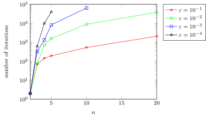
Figure 1: Number of iterations needed by Eaves’ K1 algorithm for $r=10$, and different choices of $n$ and $\varepsilon>0$ in Example 1. The maximal number of iterations was set to $10^{5}$. It took 67 seconds to generate this whole plot on an 2.4 GHz Intel MacBook.

Example 2

It is relatively easy to generate many positive $n\times n$ matrices with a specified spectral radius in MATLAB. If the spectral radius $\rho(A)$ of a nonnegative matrix $A$ is less than one then it defines a monotone mapping that should allow for a point $s^{*}\in S_{r}$ with $As^{*}\ll s^{*}$. Here we have chosen the spectral radius to be $\rho(A)=0.8$ and have generated a number of matrices $A\in\mathbb{R}^{n\times n}_{+}$ for different choices of $n$. Again we have applied the algorithm in Listing 1 and counted the number of iterations needed. The outcome is plotted in Figure 2.

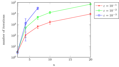
Figure 2: Mean number of iterations needed for linear maps with spectral radius $\rho(A)=0.8$ together with minimal and maximal number of iterations needed. Each data point corresponds to 10 randomly chosen matrices (using MATLAB’s rand(n)). Generating this plot took 205 seconds (not taking into account generation of the test matrices). The maximal number of iterations was set to $10^{5}$.

Example 3

Consider the monotone map $T\colon\mathbb{R}^{2}_{+}\longrightarrow\mathbb{R}^{2}_{+}$ given by $T(x)=\big{(}\sqrt{x_{2}},\lambda x_{1}^{2}\big{)}^{T}$, with $\lambda\in(0,1)$. Obviously $T(0)=0$ and it is easy to check that for any $x\in\mathbb{R}^{n}_{+}$, $T^{k}x\to 0$ as $k\to\infty$. Hence, $T$ is a contraction. Yet, given $x\in\mathbb{R}^{2}_{+}$, if not already $Tx\ll x$ then there exists no $k\geq 1$ such that $T^{k+1}x\ll T^{k}x$. For we have,

$$T^{2}x=\begin{pmatrix}\sqrt{\lambda}x_{1}\\ \lambda x_{2}\end{pmatrix},\quad Tx=\begin{pmatrix}\sqrt{x_{2}}\\ \lambda x_{1}^{2}\end{pmatrix},\quad x=\begin{pmatrix}x_{1}\\ x_{2}\end{pmatrix}.$$

Assuming that $Tx\not\ll x$, we have either $(Tx)_{1}=\sqrt{x_{2}}\geq x_{1}$, which implies $(T^{2}x)_{2}x=\lambda x_{2}\geq\lambda x_{1}^{2}=(Tx)_{2}$. Otherwise, we have $(Tx)_{2}=\lambda x_{1}^{2}\geq x_{2}$, implying that $(T^{2}x)_{1}=\sqrt{\lambda}x_{1}\geq\sqrt{x_{2}}=(Tx)_{1}$. This deduction repeats inductively. As a consequence, a pure iteration of the map $T$ cannot yield a solution to Problem 1.

7 Conclusions

- (1) Aeyels, D., De Leenheer, P.: Extension of the Perron-Frobenius theorem to homogeneous systems. SIAM J. Control Optim. 41(2), 563–582 (electronic) (2002)
- (2) Allgower, E., Georg, K.: Simplicial and continuation methods for approximating fixed points and solutions to systems of equations. SIAM Review 22, 28–85 (1980)
- (3) Allgower, E.L., Georg, K.: Numerical continuation methods, Springer Series in Computational Mathematics, vol. 13. Springer-Verlag, Berlin (1990)
- (4) Allgower, E.L., Georg, K.: Numerical path following. In: Ciarlet, P.G., Lions, J.L. (eds.) Handbook of numerical analysis., vol. V, pp. 3–207. North-Holland, Amsterdam (1997)
- (5) Eaves, B.C.: Homotopies for computation of fixed points. Math. Programming 3, 1–22 (1972)
- (6) Feoktistova, V., Matveev, A.: Dynamic interactive stabilization of the switching Kumar-Seidman system. Vestnik St. Petersburg Univ. Math. 42(3), 226–234 (2009)
- (7) Gao, K., Lin, Y.: On equivalent notions of input-to-state stability for nonlinear discrete time systems. In: Proc. of the IASTED Int. Conf. on Control and Applications, pp. 81–87 (2000)
- (8) Jiang, Z.P., Wang, Y.: Input-to-state stability for discrete-time nonlinear systems. Automatica J. IFAC 37(6), 857–869 (2001)
- (9) Karafyllis, I., Jiang, Z.P.: A vector small-gain theorem for general nonlinear control systems. Submitted to IEEE Trans. Automat. Control (2009) arXiv:0904.0755v1
- (10) Knaster, B., Kuratowski, C., Mazurkiewicz, S.: Ein Beweis des Fixpunktsatzes für -dimensionale Simplexe. Fundamenta 14, 132–137 (1929)
- (11) Krause, U.: Concave Perron-Frobenius theory and applications. Nonlinear Anal. 47(3), 1457–1466 (2001)
- (12) Lassonde, M.: Sur le principe KKM. C. R. Acad. Sci. Paris Sér. I Math. 310(7), 573–576 (1990)
- (13) Raimondo, D., Magni, L., Scattolini, R.: Decentralized MPC of nonlinear systems: An input-to-state stability approach. Int. J. Robust and Nonl. Control 17(17), 1651–1667 (2007)
- (14) Rüffer, B.S.: Monotone inequalities, dynamical systems, and paths in the positive orthant of Euclidean -space. Positivity (2010) doi:10.1007/s11117-009-0016-5 Article in press, accepted April 16, 2009
- (15) Rüffer, B.S.: Small-gain conditions and the comparison principle. IEEE Trans. Automat. Control 55(7) (2010) doi:10.1109/TAC.2010.2048053 Article in press, accepted April 1, 2010
- (16) Rüffer, B.S., Dashkovskiy, S.N.: Local ISS of large-scale interconnections and estimates for stability regions. Systems Control Lett. 59(3–4), 241–247 (2010)
- (17) Tanner, H.G., Pappas, G.J., Kumar, V.: Leader-to-formation stability. IEEE Trans. Robotics and Automation 20(3), 443–455 (2004)