An Efficient Approximation to the Correlated Nakagami-$m$ Sums and its Application in Equal Gain Diversity Receivers

Abstract

There are several cases in wireless communications theory where the statistics of the sum of independent or correlated Nakagami-$m$ random variables (RVs) is necessary to be known. However, a closed-form solution to the distribution of this sum does not exist when the number of constituent RVs exceeds two, even for the special case of Rayleigh fading. In this paper, we present an efficient closed-form approximation for the distribution of the sum of arbitrary correlated Nakagami-$m$ envelopes with identical and integer fading parameters. The distribution becomes exact for maximal correlation, while the tightness of the proposed approximation is validated statistically by using the Chi-square and the Kolmogorov-Smirnov goodness-of-fit tests. As an application, the approximation is used to study the performance of equal-gain combining (EGC) systems operating over arbitrary correlated Nakagami-$m$ fading channels, by utilizing the available analytical results for the error-rate performance of an equivalent maximal-ratio combining (MRC) system.

I Introduction

The analytical determination of the the probability distribution functions (PDF) and the cumulative distribution functions (CDF) of the sums of independent and correlated signals’ envelopes is rather cumbersome, yielding difficulties in the theoretical performance analysis of some wireless communications systems [1]. A closed-form solution for the PDF and the CDF of the sum of Rayleigh random variables (RVs) has not been presented for more then 90 years, except when the number of RVs equals two. The famous Beaulieu series for computing PDF of a sum of independent RVs were proposed in [2]. Later, a finite range multifold integral for PDF of the sum of independent and identically distributed (i.i.d.) Nakagami-$m$ RVs was proposed in [3]. A closed-form formula for the PDF of the sum of two i.i.d. Nakagami-$m$ RVs was given in [4]-[6]. Exact infinite series representations for the sum of three and four i.i.d. Nakagami-$m$ RVs was presented in [7], although their usefulness is overshadowed by their computational complexity.

The most famous application, where these sums appear, deals with the analytical performance evaluation of equal gain combining (EGC) systems [8]-[13]. Only few papers address the performance of EGC receivers in correlated fading with arbitrary-order diversity. In [14], EGC was studied by approximating the moment generating function (MGF) of the output SNR, where the moments are determined exactly only for exponentially correlated Nakagami-$m$ channels in terms of multi-fold infinite series. A completely novel approach for performance analysis of diversity combiners in equally correlated fading channels was proposed in [15], where the equally correlated Rayleigh fading channels are transformed into a set of conditionally independent Rician RVs. Based on this technique, the authors in [16] derived the moments of the EGC output signal-to-noise ratio (SNR) in equally correlated Nakagami-$m$ channels in terms of the Appell hypergeometric function, and then used them to evaluate the EGC performance metrics, such as the outage probability and the error probability (using Gaussian quadrature with weights and abscissas computed by solving sets of nonlinear equations).

All of the above works yield to results that are not expressed in closed form due to the inherent intricacy of the exact sum statistics. This intricacy can be circumvented by searching for suitable highly accurate approximations for the PDF of a sum of arbitrary number of Nakagami-$m$ RVs. Various simple and accurate approximations to the PDF of sum of independent Rayleigh, Rice and Nakagami-$m$ RVs had been proposed in [17]-[21], which had been used for analytical EGC performance evaluation. Based on the ideas given in [1], the works [18]-[21] use various alternatives of the moment matching method to arrive at the required approximation.

In this paper, we present a highly accurate closed-form approximation for the PDF of the sum of non-identical arbitrarily correlated Nakagami-$m$ RVs with identical (integer) fading parameters. By applying this approximation, we evaluate the performance of EGC systems in terms of the known performance of an equivalent maximal ratio combining (MRC) system [22], [24], thus avoiding many complex numerical evaluations inherent for the methods presented in the aforementioned previous works for the EGC performance analysis. Although approximate, the offered closed-form expressions allow to gain insight into system performance by considering, for example, operation in the low or high SNR region.

II An accurate approximation to the sum of arbitrary correlated Nakagami-$m$ envelopes

Let $Z$ be a sum of $L$ non-identical correlated Nakagami-$m$ envelopes, $\{Z_{k}\}_{k=1}^{L}$, defined as

$$Z=\sum_{k=1}^{L}Z_{k}\,.$$ (1)

The envelopes $\{Z_{k}\}_{k=1}^{L}$ are distributed according to the Nakagami-$m$ distribution, whose PDF is given by [1]

$$f_{Z_{k}}(z)=\left(\frac{m_{z}}{\Omega_{k}}\right)^{m_{z}}\frac{2z^{2m_{z}-1}}{\Gamma(m_{z})}\exp\left(-\frac{m_{z}}{\Omega_{k}}z^{2}\right),\qquad z\geq 0\,,$$ (2)

with arbitrary average powers $E[Z_{k}^{2}]=\Omega_{k}$, $1\leq k\leq L$, and the same (integer) fading parameter $m_{z}$. The power correlation coefficient between any given pair of envelopes $(Z_{i},Z_{j})$ is defined as

$$\rho_{ij}=\frac{{\rm{cov}}(Z_{i}^{2},Z_{j}^{2})}{\sqrt{{\rm{var}}(Z_{i}^{2})\ {\rm{var}}(Z_{j}^{2})}},\qquad i\neq j\,,$$ (3)

where $E[\cdot]$, $\rm{cov}(\cdot,\cdot)$ and $\rm{var}(\cdot)$ denote expectation, covariance and variance, respectively.

We propose the unknown PDF of $Z$ be approximated by the PDF of $R$ defined as

$$R=\sqrt{\sum_{k=1}^{L}R_{k}^{2}}\,\,,$$ (4)

where $R_{k}$, $1\leq k\leq L$, denote a set of $L$ correlated but identically distributed Nakagami-$m$ envelopes with same average powers, $E[R_{k}^{2}]=\Omega_{R}$, and same fading parameters, $m_{R}$. The power correlation coefficients between any given pair $(R_{i},R_{j})$ is assumed equal to that of the respective pair of the original envelopes $(Z_{i},Z_{j})$, $\rho_{ij}$.

The statistics of $R^{2}$ is easily seen to be equal to the statistics of the sum of correlated Gamma RVs. Thus, the MGF of $R^{2}$ is represented by [References, Eq. (11)]

$$M_{R^{2}}(s)=\det\left({\bf{I}}-s\frac{\Omega_{R}}{m_{R}}{\bf{\Lambda}}\right)^{-m_{R}}=\prod_{k=1}^{L}\left(1-s\frac{\Omega_{R}}{m_{R}}\lambda_{k}\right)^{-m_{R}}$$ (5)

where ${\bf{I}}$ is the $L\times L$ identity matrix and ${\bf{\Lambda}}$ is the $L\times L$ positive definite matrix (denoted as the correlation matrix) whose elements are the square roots of the power correlation coefficients,

$${\bf{\Lambda}}=\left[\begin{array}[]{ccccc}1&\sqrt{\rho_{12}}&\cdots&\sqrt{\rho_{1L}}\\ \sqrt{\rho_{21}}&1&\cdots&\sqrt{\rho_{2L}}\\ .&.&\cdots&.\\ \sqrt{\rho_{L1}}&\sqrt{\rho_{L2}}&\cdots&1\\ \end{array}\right]\,.$$ (10)

The $L$ eigenvalues of the correlation matrix ${\bf{\Lambda}}$ are denoted by $\lambda_{k}$, $1\leq k\leq L$.

Throughout literature, the PDF of $R^{2}$ is determined by using several different approaches that result in alternative closed-form solutions, two of which are given by [References, Eq. (29)] and [References, Eq. (10)]. After a simple RV transformation, these two alternatives for the PDF of $R$ are expressed as

$$f_{R}(r)=\frac{2r}{\pi}\int_{0}^{\infty}\frac{\cos\left[m_{R}\sum_{k=0}^{L-1}\arctan\left(t\frac{\Omega_{R}\lambda_{k}}{m_{R}}\right)-tr^{2}\right]}{\prod_{k=0}^{L-1}\left[1+\left(t\frac{\Omega_{R}\lambda_{k}}{m_{R}}\right)^{2}\right]^{m_{R}/2}}dt$$ (11)

$$=\frac{2r^{2Lm_{R}-1}}{\Gamma(Lm_{R})}\left(\frac{m_{R}}{\Omega_{R}}\right)^{Lm_{R}}\left(\frac{1}{\det({\bf{\Lambda}})}\right)^{m_{R}}\qquad\qquad\qquad$$

$$\times\Phi_{2}^{(L)}\left(m_{R},m_{R},\dots,m_{R};Lm_{R};-\frac{m_{R}}{\Omega_{R}}\frac{r^{2}}{\lambda_{1}},\dots,-\frac{m_{R}}{\Omega_{R}}\frac{r^{2}}{\lambda_{L}}\right),$$

(12)

where $\Phi_{2}^{(L)}(\cdot)$ is the confluent Lauricella hypergeometric function of $L$ variables, defined in [33] and [References, Eqs. (9)-(10)]. Note that (II) is here presented to demonstrate existence of an exact closed-form solution, whereas (11) is much more convenient for accurate and efficient numerical integration. For example, the PDF may be obtained using the Gauss-Legendre quadrature rule [References, Eq. (25.4.29)] over (11) [References].

Next, we apply the moment matching method to determine the parameters $\Omega_{R}$ and $m_{R}$ of the proposed approximation (11)-(II) to the PDF of $Z$. In wireless communications, moment matching methods are most typically applied to approximate distributions of the sum of log-normal RVs [29]. Most recently, a variant of moment matching, matching of the normalized first and second moments, had been applied to arrive at an improved approximation to the sum of independent Nakagami-$m$ RVs via the $\alpha$-$\mu$ distribution [20]-[21].

We arrive at required approximation by matching the first and the second moments of the powers of $Z$ and $R$, i.e., the second and fourth moments of the envelopes $Z$ and $R$,

$$E[Z^{2}]=E[R^{2}],\quad E[Z^{4}]=E[R^{4}]\,.$$ (13)

Matching the first and the second moments of the powers aids the analytical tractability of the proposed approximation due to the availability of the MGF of $R^{2}$ in closed form, given by (5). The second and the fourth moments of $R$ are determined straightforwardly by applying the moment theorem over (5), yielding

$$E[R^{2}]=\frac{dM_{R^{2}}(s)}{ds}\Bigg{|}_{s=0}=\Omega_{R}\sum_{l=1}^{L}\lambda_{l}=\Omega_{R}L\,,\qquad\quad$$ (14)

$$E[R^{4}]=\frac{d^{2}M_{R^{2}}(s)}{ds^{2}}\Bigg{|}_{s=0}=\frac{\Omega_{R}^{2}}{m_{R}}\left[\sum_{l=1}^{L}\lambda_{l}^{2}+m_{R}L^{2}\right]\,.$$ (15)

Introducing (14) and (15) into (13), one obtains the unknown parameters for the statistics of $R$

$$\Omega_{R}=\frac{E[Z^{2}]}{L}\,,\quad m_{R}=\frac{\sum_{l=1}^{L}\lambda_{l}^{2}}{L^{2}}\frac{(E[Z^{2}])^{2}}{E[Z^{4}]-(E[Z^{2}))^{2}}\,.$$ (16)

Using the multinomial theorem and [References, Eq. (137)], the second and the fourth moments of $Z$ are determined as

$$E[Z^{2}]=\sum_{k=1}^{L}\Omega_{k}+\frac{2\Gamma^{2}(m_{z}+1/2)}{m_{z}\Gamma^{2}(m_{z})}\qquad\qquad\qquad\qquad$$

$$\times\sum_{i=1}^{L}\sum_{j=i+1}^{L}\sqrt{\Omega_{i}\Omega_{j}}\,{}_{2}F_{1}\left(-1/2,-1/2;m_{z};\rho_{ij}\right),$$ (17)

$$E[Z^{4}]=\frac{m_{z}+1}{m_{z}}\sum_{m=1}^{L}\Omega_{m}^{2}+\frac{6\Gamma^{2}(m_{z}+1)}{m_{z}^{2}\Gamma^{2}(m_{z})}\sum_{i=1}^{L}\sum_{j=i+1}^{L}\Omega_{i}\Omega_{j}\qquad$$

$$\times{}_{2}F_{1}\left(-1,-1;m_{z};\rho_{ij}\right)+\frac{4\Gamma(m_{z}+3/2)\Gamma(m_{z}+1/2)}{m_{z}^{2}\Gamma^{2}(m_{z})}\qquad\quad$$

$$\times\sum_{i=1}^{L}\sum_{j=i+1}^{L}(\Omega_{i}^{3/2}\Omega_{j}^{1/2}+\Omega_{i}^{1/2}\Omega_{j}^{3/2}){}_{2}F_{1}\left(-\frac{3}{2},-\frac{1}{2};m_{z};\rho_{ij}\right)\,\,\,\,$$

$$+12\sum_{m=1}^{L}\sum_{i=m+1}^{L}\sum_{j=i+1}^{L}\Omega_{m}\sqrt{\Omega_{i}\Omega_{j}}E[Z_{m}^{2}Z_{i}Z_{j}]\qquad\qquad\qquad\quad$$

$$+12\sum_{m=1}^{L}\sum_{i=m+1}^{L}\sum_{j=i+1}^{L}\sqrt{\Omega_{m}}\Omega_{i}\sqrt{\Omega_{j}}E[Z_{m}Z_{i}^{2}Z_{j}]\qquad\qquad\quad\quad$$

$$+12\sum_{m=1}^{L}\sum_{i=m+1}^{L}\sum_{j=i+1}^{L}\sqrt{\Omega_{m}\Omega_{i}}\Omega_{j}E[Z_{m}Z_{i}Z_{j}^{2}]\qquad\qquad\qquad\quad$$

$$+\,\,\,24\sum_{m=1}^{L}\sum_{n=m+1}^{L}\sum_{i=n+1}^{L}\sum_{j=i+1}^{L}\sqrt{\Omega_{m}\Omega_{n}\Omega_{i}\Omega_{j}}E[Z_{m}Z_{n}Z_{i}Z_{j}]\,,\qquad\qquad\qquad\qquad\quad\,\,\,$$ (18)

where ${}_{2}F_{1}(\cdot)$ is the Gauss hypergeometric function [References]. The joint moments $E[Z_{m}^{2}Z_{i}Z_{j}]$, $E[Z_{m}Z_{i}^{2}Z_{j}]$, $E[Z_{m}Z_{i}Z_{j}^{2}]$ and $E[Z_{m}Z_{n}Z_{i}Z_{j}]$ are not known in closed-form for arbitrary branch correlation. Exact closed-form expressions are available only for some particular correlation models, such as the exponential and the equal correlation models. For the case or arbitrary correlation, we utilize the method presented in [27], where an arbitrary correlation matrix ${\bf{\Lambda}}$ is approximated by its respective Green’s matrix, followed by the application of the available joint moments of the exponential correlation model.

TABLE I: Fading parameter $m_{R}$ for some feasible scenarios with equal correlation

	$m_{z}=1$			$m_{z}=2$			$m_{z}=3$
$\rho$	$L=2$	$L=3$	$L=4$	$L=2$	$L=3$	$L=4$	$L=2$	$L=3$	$L=4$
	$m_{R}$	$m_{R}$	$m_{R}$	$m_{R}$	$m_{R}$	$m_{R}$	$m_{R}$	$m_{R}$	$m_{R}$
0	$0.9552$	$0.9411$	$0.9343$	$1.947$	$1.93$	$1.9217$	$2.943$	$2.9258$	$2.9168$
0.2	$0.9195$	$0.8884$	$0.8709$	$1.9102$	$1.876$	$1.8569$	$2.9068$	$2.8715$	$2.8518$
0.4	$0.9156$	$0.8841$	$0.8672$	$1.907$	$1.8722$	$1.8535$	$2.9039$	$2.868$	$2.8487$
0.6	$0.9304$	$0.9056$	$0.8929$	$1.9242$	$1.8971$	$1.8831$	$2.9222$	$2.8944$	$2.8799$
0.8	$0.9587$	$0.9445$	$0.9374$	$1.956$	$1.9409$	$1.9333$	$2.9553$	$2.9399$	$2.9321$

TABLE II: Fading parameter $m_{R}$ for some feasible scenarios with exponential correlation

	$m_{z}=1$			$m_{z}=2$			$m_{z}=3$
$\rho$	$L=2$	$L=3$	$L=4$	$L=2$	$L=3$	$L=4$	$L=2$	$L=3$	$L=4$
	$m_{R}$	$m_{R}$	$m_{R}$	$m_{R}$	$m_{R}$	$m_{R}$	$m_{R}$	$m_{R}$	$m_{R}$
0	$0.9552$	$0.9411$	$0.9343$	$1.947$	$1.93$	$1.9217$	$2.943$	$2.9258$	$2.9168$
0.2	$0.9195$	$0.9033$	$0.9015$	$1.9102$	$1.892$	$1.8897$	$2.9068$	$2.8878$	$2.8852$
0.4	$0.9156$	$0.8887$	$0.88$	$1.907$	$1.877$	$1.8675$	$2.9039$	$2.8728$	$2.8629$
0.6	$0.9304$	$0.8988$	$0.8817$	$1.9242$	$1.889$	$1.87$	$2.9222$	$2.8858$	$2.866$
0.8	$0.9587$	$0.934$	$0.9162$	$1.956$	$1.9291$	$1.9093$	$2.9553$	$2.9277$	$2.9072$

II-A Equal correlation model

Equal correlation typically corresponds to the scenario of multichannel reception from closely spaced diversity antennas (e.g., three antennas placed on an equilateral triangle). This model may be employed as a worst case correlation scenario, since the impact of correlation on system performance for other correlation models typically will be less severe [22], [30].

For this correlation model, the power correlation coefficients are all equal,

$$\rho_{ij}=\rho,\quad i\neq j,\quad 0\leq\rho\leq 1\,.$$ (19)

When $m_{z}$ is assumed to be integer, the unknown joint moments in (II) can be expressed in closed-form as [References, Eq. (43)]

$$E[Z_{m}^{2}Z_{i}Z_{j}]=E[Z_{m}Z_{i}^{2}Z_{j}]=E[Z_{m}Z_{i}Z_{j}^{2}]\qquad\qquad$$

$$=\left(\frac{1-\sqrt{\rho}}{m_{z}}\right)^{2}W(2,1,1)\,\,,\qquad\qquad$$ (20)

$$E[Z_{m}Z_{n}Z_{i}Z_{j}]=\left(\frac{1-\sqrt{\rho}}{m_{z}}\right)^{2}W(1,1,1,1)\,,\qquad\quad$$ (21)

where the coefficients $W(\cdots)$ are determined as

$$W(k_{1},...,k_{N})=\left(\prod_{j=1}^{N}\frac{\Gamma(m_{z}+k_{j}/2)}{\Gamma(m_{z})}\right)\left(\frac{1-\sqrt{\rho}}{1+(N-1)\sqrt{\rho}}\right)^{m_{z}}$$

$$\times F_{A}^{(N)}\left(m_{z};m_{z}+\frac{k_{1}}{2},\cdots,m_{z}+\frac{k_{N}}{2};m_{z},\cdots,m_{z};\right.\qquad\qquad$$

$$\left.\frac{\sqrt{\rho}}{1+(N-1)\sqrt{\rho}},\cdots,\frac{\sqrt{\rho}}{1+(N-1)\sqrt{\rho}}\right)\,,$$ (22)

with $F_{A}^{(N)}(\cdot)$ denoting the Lauricella $F_{A}$ hypergeometric function of $N$ variables, defined by [References, Eq. (9.19)] and [References, Eqs. (11)-(13)].

Note that the coefficient $W(2,1,1)$ needs to be evaluated when $L\geq 3$, whereas the coefficient $W(1,1,1,1)$ needs to be evaluated when $L\geq 4$. In Appendix A, $W(2,1,1)$ is reduced to the more familiar hypergeometric functions, attaining the form given by (A). $W(1,1,1,1)$ requires numerical evaluation of the Lauricella $F_{A}$ function of 4 variables, which can be computed with desired accuracy by using one of the two numerical methods presented in [References, Section IV.A].

The assumption of equal average powers, $\Omega_{k}=\Omega_{Z}$, $1\leq k\leq L$, yields independence of $m_{R}$ from $\Omega_{Z}$. For this case, Table I gives the values of $m_{R}$ for several combinations of $\rho$, $L$ and $m_{Z}$. The use of Table I aids the practical applicability of our approach for the case of equal average powers.

For the equal correlation model, the eigenvalues of ${\bf{\Lambda}}$ are exactly found as $\lambda_{1}=1+(L-1)\sqrt{\rho}$ and $\lambda_{k}=(1-\sqrt{\rho})$ for $2\leq k\leq L$, so the statistics of $R^{2}$ is identical to that of the sum of a pair of independent Nakagami RVs. Thus, the MGF of $R^{2}$ is given by [References, Eq. (9.213)], whereas the PDF of $R$ is given by [References, Eq. (9.208)]

$$f_{R}(r)=\left(\frac{m_{R}}{\Omega_{R}}\right)^{m_{R}L}\qquad\qquad\qquad\qquad\qquad\qquad\qquad$$

$$\times\frac{2r^{2m_{R}L-1}\exp\left({-m_{R}r^{2}}/{((1-\sqrt{\rho})\Omega_{R}})\right)}{\Gamma(m_{R}L)(1-\sqrt{\rho})^{m_{R}(L-1)}(1+(L-1)\sqrt{\rho})^{m_{R}}}\qquad$$

$$\times{}_{1}F_{1}\left(m_{R};m_{R}L;\frac{m_{R}L\sqrt{\rho}}{(1-\sqrt{\rho})(1+(L-1)\sqrt{\rho})\Omega_{R}}r^{2}\right),$$ (23)

where ${}_{1}F_{1}(\cdot)$ is the Kummer confluent hypergeometric function [References, Eq. (9.210)].

II-B Exponential correlation model

Exponential correlation typically corresponds to the scenario of multichannel reception from equispaced diversity antennas in which the correlation between the pairs of combined signals decays as the spacing between the antennas increases [22], [30].

For this correlation model, the power correlation coefficients are determined as

$$\rho_{ij}=\rho^{|i-j|},\qquad 0\leq\rho\leq 1\,.$$ (24)

The unknown joint moments in (II), $E[Z_{m}^{2}Z_{i}Z_{j}]$, $E[Z_{m}Z_{i}^{2}Z_{j}]$, $E[Z_{m}Z_{i}Z_{j}^{2}]$ and $E[Z_{m}Z_{n}Z_{i}Z_{j}]$, can be calculated from [References, Eqs. (11) and (12)]. The Appendix B derives simpler alternatives to [References, Eqs. (11) and (12)], which involve a single infinite sum and a familiar hypergeometric function,

$$E[Z_{m}^{n_{1}}Z_{i}^{n_{2}}Z_{j}^{n_{3}}]=\frac{|{\bf{\Delta}}|^{m_{z}}}{\delta_{11}^{m_{z}+n_{1}/2}\delta_{22}^{m_{z}+n_{2}/2}\delta_{33}^{m_{z}+n_{3}/2}}\qquad\qquad$$

$$\times\,\frac{\Gamma(m_{z}+n_{3}/2)}{\Gamma^{2}(m_{z})m_{z}^{(n_{1}+n_{2}+n_{3})/2}}\,\sum_{k=0}^{\infty}\left(\frac{\delta_{12}^{2}}{\delta_{11}\delta_{22}}\right)^{k}\qquad\,$$

$$\times\,\frac{\Gamma(m_{z}+k+n_{1}/2)\Gamma(m_{z}+k+n_{2}/2)}{\Gamma(m_{z}+k)k!}\qquad\quad$$

$$\times{}_{2}F_{1}\left(m_{z}+k+\frac{n_{2}}{2},m_{z}+\frac{n_{3}}{2},m_{z},\frac{\delta_{23}^{2}}{\delta_{22}\delta_{33}}\right),\,$$ (25)

$$E[Z_{m}Z_{n}Z_{i}Z_{j}]=\frac{|{\bf{\Psi}}|^{m_{z}}}{(\psi_{11}\psi_{22}\psi_{33}\psi_{44})^{m_{z}+1/2}}\frac{\Gamma^{2}(m_{z}+1/2)}{\Gamma^{3}(m_{z})m_{z}^{2}}$$

$$\times\sum_{k=0}^{\infty}\frac{\Gamma^{2}(m_{z}+k+1/2)}{k!\Gamma(m_{z}+k)}\left(\frac{\psi_{23}^{2}}{\psi_{22}\psi_{33}}\right)^{k}\qquad\,\,\,$$

$$\times\,{}_{2}F_{1}\left(m_{z}+\frac{1}{2},k+m_{z}+\frac{1}{2},m_{z},\frac{\psi_{12}^{2}}{\psi_{11}\psi_{22}}\right)$$

$$\times{}_{2}F_{1}\left(m_{z}+\frac{1}{2},k+m_{z}+\frac{1}{2},m_{z},\frac{\psi_{34}^{2}}{\psi_{33}\psi_{44}}\right).$$ (26)

In (II-B), $(n_{1},n_{2},n_{3})$ = $(2,1,1)$ for the calculation of $E[Z_{m}^{2}Z_{i}Z_{j}]$, $(n_{1},n_{2},n_{3})$ = $(1,2,1)$ for the calculation of $E[Z_{m}Z_{i}^{2}Z_{j}]$ and $(n_{1},n_{2},n_{3})$ = $(1,1,2)$ for the calculation of $E[Z_{m}Z_{i}Z_{j}^{2}]$. The matrix ${\bf{\Delta}}=[\delta_{i,j}]$ is the inverse of ${\bf{\Lambda}}$’s principal submatrix composed of the $m$-th, $i$-th and $j$-th rows and columns of ${\bf{\Lambda}}$, whereas the matrix ${\bf{\Psi}}=[\psi_{i,j}]$ is the inverse of ${\bf{\Lambda}}$’s principal submatrix composed of the $m$-th, $n$-th, $i$-th and $j$-th rows and columns of ${\bf{\Lambda}}$,

$${\bf{\Delta}}=\left[\begin{array}[]{ccccc}1&\sqrt{\rho_{mi}}&\sqrt{\rho_{mj}}\\ \sqrt{\rho_{im}}&1&\sqrt{\rho_{ij}}\\ \sqrt{\rho_{jm}}&\sqrt{\rho_{ji}}&1\\ \end{array}\right]^{-1},$$

$${\bf{\Psi}}=\left[\begin{array}[]{ccccc}1&\sqrt{\rho_{mn}}&\sqrt{\rho_{mi}}&\sqrt{\rho_{mj}}\\ \sqrt{\rho_{nm}}&1&\sqrt{\rho_{ni}}&\sqrt{\rho_{nj}}\\ \sqrt{\rho_{im}}&\sqrt{\rho_{in}}&1&\sqrt{\rho_{ij}}\\ \sqrt{\rho_{jm}}&\sqrt{\rho_{jm}}&\sqrt{\rho_{ji}}&1\\ \end{array}\right]^{-1}\,.$$ (32)

The exactness of (II-B)-(II-B) arise from the fact that both matrices ${\bf{\Delta}}$ and ${\bf{\Psi}}$ are tridiagonal matrices due to (24) [References, Section IV]. Introducing (II-B)-(II-B) into (II), one obtains the closed-form expression for $E[Z^{4}]$, which is omitted here for brevity. Combining (II)-(II) into (16), one obtains the unknown parameters $\Omega_{R}$ and $m_{R}$ for the statistics of $R$.

The assumption of equal average powers, $\Omega_{k}=\Omega_{Z}$, $1\leq k\leq L$, again renders independence of $m_{R}$ from $\Omega_{Z}$ for the exponential correlation model. Under such assumptions, Table II displays the values of $m_{R}$ for several illustrative combinations of $\rho$, $L$ and $m_{Z}$.

II-C Arbitrary correlation model

In the general case of arbitrary branch correlations, the correlation matrix ${\bf{\Lambda}}$ is approximated by its appropriate Green’s matrix, ${\bf{C}}$, utilizing the method presented in [References, Section IV]. Since principal submatrices of Green’s matrices are also Green’s matrices, the matrices ${\bf{\Delta}}$ and ${\bf{\Psi}}$, defined by (II-B), are determined to be tridiagonal, yielding direct applicability of the results presented in Section II.B to determine the unknown parameters $\Omega_{R}$ and $m_{R}$ for the statistics of $R$. Thus, the statistics of $Z$ are approximated by the statistics of $R$, whose arbitrary correlation matrix ${\bf{\Lambda}}$ is approximated by the Green’s matrix ${\bf{C}}$. In the following subsection, we illustrate the highly accurate approximation to the PDF of $Z$ facilitated by this approach.

TABLE III:                   Significance levels of C-S and K-S tests for goodness
of fit between the exact and the approximative distributions of Fig. 1

	$m_{z}=1$				$m_{z}=3$
$\rho$	$L=2$		$L=5$		$L=2$		$L=5$
	$\alpha_{CS}$	$\alpha_{KS}$	$\alpha_{CS}$	$\alpha_{KS}$	$\alpha_{CS}$	$\alpha_{KS}$	$\alpha_{CS}$	$\alpha_{KS}$
0.2	$0.004$	$0.02$	$0.17$	$0.06$	$<0.001$	$<0.001$	$<0.001$	$<0.001$
0.7	$0.04$	$0.03$	$0.2$	$0.18$	$<0.001$	$<0.001$	$<0.001$	$<0.001$

TABLE IV:                   Significance levels of C-S and K-S tests for goodness
of fit between the exact and the approximative distributions of Fig. 2

	$m_{z}=1$				$m_{z}=3$
$\rho$	$L=2$		$L=5$		$L=2$		$L=5$
	$\alpha_{CS}$	$\alpha_{KS}$	$\alpha_{CS}$	$\alpha_{KS}$	$\alpha_{CS}$	$\alpha_{KS}$	$\alpha_{CS}$	$\alpha_{KS}$
0.2	$<0.001$	$0.02$	$<0.001$	$<0.001$	$<0.001$	$<0.001$	$<0.001$	$<0.001$
0.7	$0.08$	$0.04$	$0.02$	$0.17$	$<0.001$	$<0.001$	$<0.001$	$<0.001$

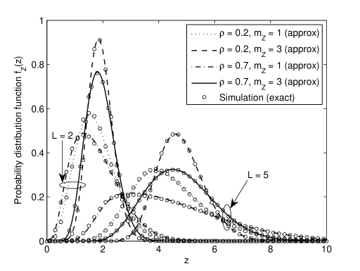
Figure 1: Exact (obtained by simulation) and the approximative analytical PDFs to the sum of equally correlated Nakagami-$m$ RVs with equal average powers, when $\Omega_{Z}=1$

II-D Validation via statistical goodness-of-fit tests

We now statistically validate the proposed PDF approximations for equal, exponential and arbitrary branch correlation by using two different goodness-of-fit tests. The Chi-square (C-S) and Kolmogorov-Smirnov (K-S) tests provide two different statistical metrics, $\chi_{n}^{2}$ and $D_{n}$, which describe the discrepancy between the observed samples of $Z$ and the samples expected under the analytical distribution (11)-(II).

Each metric is averaged over 100 statistical samples, where each statistical sample comprises of 10000 independent random samples of $Z$. The random samples of $Z$ are generated by computer simulations of correlated Nakagami-$m$ RVs based on the method proposed in [References, Section VII].

For each metric, we calculate the significance level $\alpha$ from the C-S and K-S distributions, respectively denoted as $\alpha_{CS}$ and $\alpha_{KS}$. The significance level $\alpha$ represents the probability of rejecting the tested null hypothesis ($H_{0}$: ”the random samples of $Z$, obtained from (1), belong to the distribution given by (11)-(II)”), when it is actually true. The small values of $\alpha$ indicate a good fit.

Note that, significance levels $\alpha$ less then $0.2$ still indicate a good fit, due to the rigourousness of both C-S and K-S tests in accepting the null hypothesis $H_{0}$.

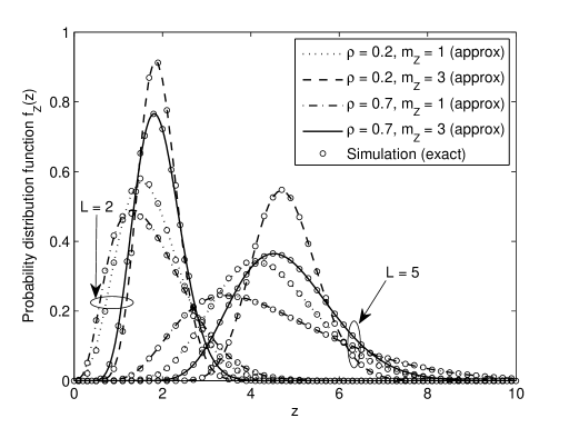
Figure 2: Exact (obtained by simulation) and the approximative analytical PDFs to the sum of exponentially correlated Nakagami-$m$ RVs with equal average powers, when $\Omega_{Z}=1$

II-D1 Equal and exponential correlation

For the equal and exponential correlation models, the goodness-of-fit testing is conducted for combinations of the followings input parameters: $L=2$ and $5$, $m_{Z}=1$ and $3$, $\rho=0.2$ and $0.7$, whereas the average powers of $Z_{k}$ are assumed equal to unity ($\Omega_{Z}=1$). The needed fading parameter $m_{R}$ of distribution (11)-(II) is obtained directly from Tables I and II, whereas the average power $\Omega_{R}$ is calculated from (16).

Figs. 1 and 2 depict the excellent (visual) match between the histogram obtained from generated samples of $Z$ and the proposed approximation, for the cases of equal and exponential correlation models, respectively. Tables III and IV complement Figs. 1 and 2, by presenting the significance levels $\alpha$ for the corresponding input parameters’ combinations. The Table III and the Table IV entries reveal the very low significance levels $\alpha$ for all input parameters’ combinations, thus proving an excellent goodness of fit in statistical sense.

II-D2 Arbitrary correlation

For illustrative purposes, we use same two example correlation matrices from [References, Sections V.B and V.D], $\Sigma_{3\_\rm{lin}}$ and $\Sigma_{4\_\rm{circ}}$, here denoted as ${\bf{\Lambda_{1}}}$ and ${\bf{\Lambda_{2}}}$, respectively. They are approximated by their Green’s matrices $C_{3\_\rm{lin}}$ and $C_{4\_\rm{circ}}$, here denoted as ${\bf{C_{1}}}$ and ${\bf{C_{2}}}$, respectively.

Using ${\bf{C_{1}}}$ and ${\bf{C_{2}}}$, one obtains the needed tridiagonal matrices ${\bf{\Delta}}$ and ${\bf{\Psi}}$ from their definitions given by (II-B). The required joint moments are then calculated from (II-B) and (II-B), which are then substituted into (II) and (II) to calculate $E[Z^{2}]$ and $E[Z^{4}]$, and then (16) is used to describe the statistics of $R$.

TABLE V: Significance levels of C-S and K-S tests for goodness of fit between exact and approximative distributions of Fig. 3

	$m_{z}=1$		$m_{z}=3$
	$\alpha_{CS}$	$\alpha_{KS}$	$\alpha_{CS}$	$\alpha_{KS}$
$\Lambda_{1}$	$0.19$	$0.18$	$<0.001$	$<0.001$
$\Lambda_{2}$	$0.12$	$0.11$	$<0.001$	$<0.001$

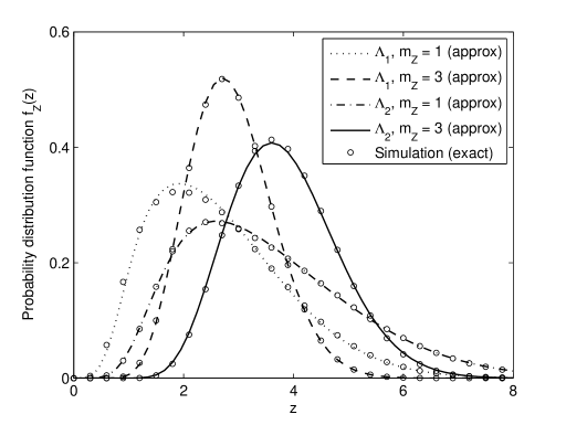
Figure 3: Exact (obtained by simulation) and the approximative analytical PDFs to the sum of correlated Nakagami-$m$ RVs with equal average powers, when $\Omega_{Z}=1$), and correlation matrices ${\bf{\Lambda_{1}}}$ and ${\bf{\Lambda_{2}}}$

Fig. 3 depicts the excellent (visual) match between the histogram obtained from generated samples of $Z$ and the proposed approximation (11)-(II), for the two example correlation matrices $\Lambda_{1}$ and $\Lambda_{2}$. Table V complements Figs. 3, by revealing the very low significance levels $\alpha_{s}$, thus again proving an excellent goodness of fit.

II-E Validation in case of maximal correlation

We now consider the case of maximal correlation coefficient between any pair of Nakagami-$m$ envelopes $Z_{i}$ and $Z_{j}$, i.e., $\rho_{ij}=1$. It indicates a perfect linear relationship between these pairs, which, after applying the model from [References, Eq. (37)], can be defined as $Z_{i}=\sqrt{\Omega_{i}}\,Z_{0}$ for $1\leq i\leq L$, where $Z_{0}$ is an auxiliary Nakagami-$m$ RV with unity average power and same fading parameter $m_{z}$. After replacing the latter expression into (1), $Z$ is transformed into a Nakagami-$m$ RV with fading parameter $m_{z}$ and average power of

$$E[Z^{2}]=\left(\sum_{i=1}^{L}\sqrt{\Omega_{i}}\right)^{2}=\sum_{i=1}^{L}\sum_{j=1}^{L}\sqrt{\Omega_{i}\Omega_{j}}\,,$$ (33)

which agrees with (II) when $\rho_{ij}\rightarrow 1$.

Replacing $\rho_{ij}=1$ into (10), the $L-1$ eigenvalues of the matrix $\bf{\Lambda}$ turn up equal to 0, except $\lambda_{1}=L$. After plugging these eigenvalues into (5), $R$ is transformed into a Nakagami-$m$ RV with fading parameter $m_{R}$ and average power $L\Omega_{R}$. After the moment matching, $\Omega_{R}$ and $m_{R}$ can be obtained from (16), as

$$\Omega_{R}=\frac{1}{L}\sum_{i=1}^{L}\sum_{j=1}^{L}\sqrt{\Omega_{i}\Omega_{j}},\quad m_{R}=\frac{(E[Z^{2}])^{2}}{E[Z^{4}]-(E[Z^{2}])^{2}}=m_{z}\,,$$ (34)

respectively, where the latter equality is attributed to the definition of the Nakagami-$m$ fading parameter, given by [References, Eq. (4)].

Thus, maximal correlation yields (11)-(II) as an accurate distribution of $Z$, when our moment matching approach is applied. This conclusion further validates our approach.

III Application to the performance analysis of EGC receivers

We now consider a typical $L$-branch EGC diversity receiver exposed to slow and flat Nakagami-$m$ fading. The envelopes of the branch signals $Z_{k}$ are non-identical correlated Nakagami-$m$ random processes with PDFs given by (2), whereas their respective phases are i.i.d. uniform random processes. Each branch is also corrupted by additive white Gaussian noise (AWGN) with power spectral density $N_{0}/2$, which is added to the useful branch signal. In the EGC receiver, the random phases of the branch signals are compensated (co-phased), equally weighted and then summed together to produce the decision variable. The envelope of the composite useful signal, denoted by $Z$, is given by (1), whereas the composite noise power is given by $\sigma_{EGC}^{2}=LN_{0}/2$, resulting in the instantaneous output SNR given by

$$\gamma_{EGC}=\frac{Z^{2}}{2\sigma_{EGC}^{2}}=\frac{1}{LN_{0}}\left(\sum_{k=1}^{L}Z_{k}\right)^{2}=\left(\sum_{k=1}^{L}G_{k}\right)^{2}$$ (35)

where RVs $G_{k}=Z_{k}/\sqrt{LN_{0}}$, $1\leq k\leq L$, form a set of $L$ non-identical equally correlated Nakagami-$m$ RVs with $E[G_{k}^{2}]=\bar{\gamma}_{k}/L$, same fading parameters $m_{Z}$ and correlation coefficient $\rho_{ij}$ between branch pair $(i,j)$. Note that $\bar{\gamma}_{k}=\Omega_{k}/N_{0}$ denotes the average SNR in $k$-th branch.

Using the results from Section II, the MGF and the PDF of (35) can be approximated using (5) and (11)-(II), respectively, when $\Omega_{R}$ is replaced by $\bar{\gamma}_{R}=\Omega_{R}/(LN_{0})$. These approximations are then used to determine the outage probability $F_{\gamma_{EGC}}$ and the error probability $\bar{P}_{EGC}$ of an $L$-branch EGC systems in correlated Nakagami-$m$ fading with high accuracy.

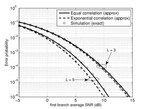
Figure 4: Exact and approximate error probabilities of an EGC receiver with correlated Nakagami-$m$ branches, when $m_{z}=2$, $\mu=0$ and $\rho=0.7$

III-A Outage probability

The outage probability of the EGC system with arbitrary correlated Nakagami-$m$ fading branches, whose output SNR drops below threshold $t$, is approximated by the known outage probability expressions of an equivalent MRC system [References, Eq. (28)], [References, Eq. (13)],

$$F_{\gamma_{EGC}}(t)\approx F_{\gamma_{MRC}}(t)\qquad\qquad\qquad\qquad\qquad\qquad\qquad$$

$$=\frac{1}{2}-\frac{1}{\pi}\int_{0}^{\infty}\frac{\sin\left[m_{R}\sum_{k=0}^{L-1}\arctan\left(x\frac{\Omega_{R}\lambda_{k}}{m_{R}}\right)-xt\right]}{\prod_{k=0}^{L-1}\left[1+\left(x\frac{\Omega_{R}\lambda_{k}}{m_{R}}\right)^{2}\right]^{m_{R}/2}}\frac{dx}{x}$$

$$=\frac{1}{\Gamma(1+Lm_{R})}\left(\frac{m_{R}}{\Omega_{R}}t\right)^{Lm_{R}}\frac{1}{\det(\Lambda)}\qquad\qquad\qquad\qquad$$

$$\times\Phi_{2}^{(L)}\Big{(}m_{R},m_{R},\dots,m_{R};1+Lm_{R};\qquad\qquad\qquad$$

$$\left.-\frac{m_{R}}{\Omega_{R}\lambda_{1}}t,-\frac{m_{R}}{\Omega_{R}\lambda_{2}}t,\dots,-\frac{m_{R}}{\Omega_{R}\lambda_{L}}t\right)\,.$$ (36)

For the equal correlation model, (III-A) can be simplified using [References, Eq. (2.1.3(1))].

III-B Average error probability

The average error probability of the correlated Nakagami-$m$ EGC system with BPSK modulation / coherent demodulation is approximated using the available expressions for the average error probability of the equivalent MRC systems. Based on [References, Eq. (9.11)] and [References, Eq. (17)], the error performance of this EGC system is alternatively approximated as

$$\bar{P}_{EGC-BPSK}\approx\bar{P}_{MRC-BPSK}=\frac{1}{\pi}\int_{0}^{\pi/2}M_{R^{2}}\left(\frac{-1}{\sin^{2}\theta}\right)d\theta$$ (37)

$$=\frac{\Gamma(Lm_{R}+1/2)}{2\sqrt{\pi}\Gamma(Lm_{R}+1)}\left(\frac{m_{R}}{\Omega_{R}}\right)^{Lm_{R}}\left(\frac{1}{\det(\Lambda)}\right)^{m_{R}}\qquad\quad$$

$$\times\,F_{D}^{(L)}\Big{(}Lm_{R}+1/2,m_{R},\dots,m_{R};Lm_{R}+1;$$

$$\left.-\frac{m_{R}}{\Omega_{R}\lambda_{1}},-\frac{m_{R}}{\Omega_{R}\lambda_{2}},\dots,-\frac{m_{R}}{\Omega_{R}\lambda_{L}}\right)\,.$$ (38)

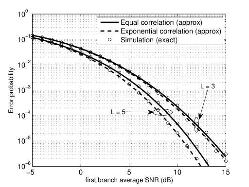
Figure 5: Exact and approximate error performance of an EGC receiver with correlated Nakagami-$m$ branches, when $m_{z}=2$, $\mu=0.3$ and $\rho=0.7$

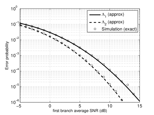
Figure 6: Exact and approximate error performance of an EGC receiver with correlated Nakagami-$m$ branches, when correlation is described by correlation matrices ${\bf{\Lambda_{1}}}$ and ${\bf{\Lambda_{2}}}$, $m_{z}=2$ and $\mu=0$

In (37), $M_{R^{2}}(\cdot)$ is replaced with the MGF given by (5). In (38), $F_{D}^{(L)}(\cdot)$ denotes the Lauricella $F_{D}$ hypergeometric function of $L$ variables, defined in [33] and [References, Eq. (18)]. For the equal correlation model, the average error probability can be calculated using [References, Eq. (32)], which is a special case of (38).

Note that (38) is here presented to demonstrate existence of an exact closed-form solution, whereas (37) is much more convenient for accurate and efficient numerical integration. For example, the average error probability may be obtained by applying the Gauss-Chebyshev quadrature rule [References, Eq. (25.4.38)] over (37). In the case of the balanced diversity branches with equal or exponential correlation, the combination of this quadrature rule with Tables I and II allows efficient and extremely accurate evaluation of the EGC performance.

The average error probability of correlated Nakagami-$m$ EGC system with BFSK modulation / non-coherent demodulation is approximated by known expression of the equivalent MRC system [References, Eq. (16)], $\bar{P}_{EGC-BFSK}\approx\bar{P}_{MRC-BFSK}=\frac{1}{2}\,M_{R^{2}}(-\frac{1}{2})$, where $M_{R^{2}}(\cdot)$ is given by (5).

III-C Validation via Monte-Carlo simulations

Next, we illustrate the tightness of the error performance of an correlated Nakagami-$m$ EGC system with BPSK modulation / coherent demodulation to that of the equivalent MRC system. The results for the actual EGC system are obtained by Monte-Carlo simulations, whereas those of the equivalent MRC system are obtained using (37).

III-C1 Equal and exponential branch correlation

Figs. 4 and 5 displays the comparative error performance of the actual EGC and the equivalent MRC systems, for several combinations of $(\rho,L,m_{Z},\Omega_{k})$. In order to accommodate unequal average branch powers (thus, unequal average branch SNRs), we used the exponentially decaying profile, modelled as

$$\Omega_{k}=\Omega_{1}\exp(-\mu(k-1)),\quad 1\leq k\leq L\,,$$ (39)

where $\Omega_{1}$ is the average power of branch 1 and $\mu$ is the decaying exponent, with $\mu=0$ denoting the case of branches with equal power (i.e., the balanced branches).

III-C2 Arbitrary branch correlation

Fig. 6 depicts the comparative error performances of the EGC with same correlation matrices from Section II.D, ${\bf{\Lambda_{1}}}$ and ${\bf{\Lambda_{2}}}$, and the equivalent MRC system with respective Green’s matrices ${\bf{C_{1}}}$ and ${\bf{C_{2}}}$. The high accuracy of our approach is maintained for arbitrary branch correlations.

IV Conclusions

A tight closed-form approximation to the distribution of the sum of correlated Nakagami-$m$ RVs was introduced for the case of identical and integer fading parameters. The proposed method approximates this distribution by using the statistics of the square-root of the sum of statistically independent Gamma RVs. Examples indicate that the new approximation is highly accurate over the entire range of abscissas. To demonstrate this more rigorously, the proposed distribution is tested against the computer generated data by the use of the Chi-square and the Kologorov-Smirnov goodness-of-fit tests. In case of maximal correlation, the proposed distribution becomes the exact distribution.

The presented approach allowed to successfully tackle the famous problem of analytical performance evaluation of an EGC system with arbitrarily correlated and unbalanced Nakagami-$m$ branches. The significance of the presented results is underpinned by the existence of a large body of literature dealing with MRC performance analysis, which permits highly accurate and efficient EGC performance evaluation.

Appendix A

Using [References, Eqs. (9.212 (1)) and (7.622 (1))], one has the following identity

$$J(m,a,p,q)=\frac{1}{\Gamma(m)}\quad\qquad\qquad\qquad\qquad\qquad\qquad\qquad\quad$$

$$\times\int_{0}^{\infty}u^{m-1}e^{-u}{}_{1}F_{1}\left(-\frac{p}{2};m;-au\right){}_{1}F_{1}\left(-\frac{q}{2};m;-au\right)du$$

$$=(1+a)^{\frac{p}{2}}\left(\frac{1+2a}{1+a}\right)^{\frac{q}{2}}{}_{2}F_{1}\left(m+\frac{p}{2},-\frac{q}{2};m;-\frac{a^{2}}{1+2a}\right)$$ (A.1)

Using [References, Eq. (9.212 (3)), pp. 1023] with some simple algebraic manipulations, the general form (II-A) of the coefficient $W(2,1,1)$ can be simplified as

$$W(2,1,1)=m_{z}\left(\frac{\Gamma(m_{z}+1/2)}{\Gamma(m_{z})}\right)^{2}\left(\frac{1-\sqrt{\rho}}{1+(N-1)\sqrt{\rho}}\right)^{m_{z}}$$

$$\times\bigg{[}J(m_{z},a,1,1)+\frac{a(m_{z}+1/2)^{2}}{m_{z}^{2}}\qquad\qquad\qquad\qquad\quad$$

$$\times\,J(m_{z}+1,a,1,1)+\frac{a}{4m_{z}^{2}}J(m_{z}+1,a,-1,-1)$$

$$-\frac{a(m_{z}+1/2)^{2}}{m_{z}^{2}}J(m_{z}+1,a,-1,1)\bigg{]}$$

(A.2)

where $a=\sqrt{\rho}/(1+(N-1)\sqrt{\rho})$

Appendix B

The unknown joint moments in (II), $E[Z_{m}^{2}Z_{i}Z_{j}]$, $E[Z_{m}Z_{i}^{2}Z_{j}]$, $E[Z_{m}Z_{i}Z_{j}^{2}]$ and $E[Z_{m}Z_{n}Z_{i}Z_{j}]$ can be calculated from [References, Eqs. (11) and (12)]. Here we derive their simpler and computationally more efficient alternatives. The alternative to [References, Eq. (12)] is derived directly from the definition of the joint moment $E[Z_{1}Z_{2}Z_{3}Z_{4}]$,

$$E[Z_{m}Z_{n}Z_{i}Z_{j}]=\int_{0}^{\infty}\int_{0}^{\infty}\int_{0}^{\infty}\int_{0}^{\infty}z_{m}z_{n}z_{i}z_{j}\qquad$$

$$\times f_{Z_{m}Z_{n}Z_{i}Z_{j}}(z_{m},z_{n},z_{i},z_{j})dz_{m}dz_{n}dz_{i}dz_{j}\,,$$ (B.1)

where joint pdf of four exponentially correlated Nakagami-$m$ RVs is expressed as [References, Eq. (9)]

$$f_{Z_{m}Z_{n}Z_{i}Z_{j}}(z_{m},z_{n},z_{i},z_{j})\qquad\qquad\qquad\qquad\qquad\quad$$

$$=\frac{2^{4}m_{z}^{m_{z}+3}|{\bf{\Psi}}|^{m_{z}}}{\Gamma(m_{z})}\frac{z_{m}^{m_{z}}z_{n}z_{i}z_{j}^{m_{z}}}{|\psi_{12}\psi_{23}\psi_{34}|^{m_{z}-1}}\qquad\qquad\quad$$

$$\times I_{m_{z}-1}\left(2m_{z}|\psi_{12}|z_{m}z_{n}\right)I_{m_{z}-1}\left(2m_{z}|\psi_{23}|z_{n}z_{i}\right)$$

$$\times I_{m_{z}-1}(2m_{z}|\psi_{34}|z_{i}z_{j})\,\exp\Big{(}-m_{z}\big{(}\psi_{11}z_{m}^{2}\qquad$$

$$+\psi_{22}z_{n}^{2}+\psi_{33}z_{i}^{2}+\psi_{44}z_{j}^{2}\big{)}\Big{)},$$ (B.2)

where ${\bf{\Psi}}=[\psi_{i,j}]$ is defined by (32). Now, we integrate [References, Eq. (11)] over $z_{m}$ and $z_{j}$, respectively obtaining

$$\int_{0}^{\infty}z_{m}^{m_{z}+1}\exp\left(-m_{z}\psi_{11}z_{m}^{2}\right)I_{m_{z}-1}\left(2m_{z}\psi_{12}z_{m}z_{n}\right)$$

$$=\frac{1}{2}\left(m_{z}\psi_{12}z_{n}\right)^{m_{z}-1}\left(m_{z}\psi_{11}\right)^{-(m_{z}+1/2)}\qquad\qquad$$

$$\times\frac{\Gamma(m_{z}+1/2)}{\Gamma(m_{z})}{}_{1}F_{1}\left(m_{z}+\frac{1}{2};m_{z};m_{z}\frac{\psi_{12}^{2}}{\psi_{11}}z_{n}^{2}\right),$$ (B.3)

and

$$\int_{0}^{\infty}z_{j}^{m_{z}+1}\exp\left(-m_{z}\psi_{44}z_{j}^{2}\right)I_{m_{z}-1}\left(2m_{z}\psi_{34}z_{i}z_{j}\right)$$

$$=\frac{1}{2}\left(m_{z}\psi_{34}z_{n}\right)^{m_{z}-1}\left(m_{z}\psi_{44}\right)^{-(m_{z}+1/2)}\qquad\qquad$$

$$\times\frac{\Gamma(m_{z}+1/2)}{\Gamma(m_{z})}{}_{1}F_{1}\left(m_{z}+\frac{1}{2};m_{z};m_{z}\frac{\psi_{34}^{2}}{\psi_{44}}z_{i}^{2}\right)\,.$$ (B.4)

We then use the series expansion of the modified Bessel function of first kind [References, Eq. (8.445)] that allows to separate the integrations per variables $z_{n}$ and $z_{i}$, yielding (II-B). A similar procedure yields to an alternative of [References, Eq. (11)] given by (II-B).

References

• [1] M. Nakagami, β€œThe $m$-distribution A general formula of intensity distribution of rapid fading,” Statistical Methods in Radio Wave Propagation, W. G. Hoffman, Ed. Oxford, U.K.: Pergamon, 1960.
• [2] N. C. Beaulieu, β€œAn infinite series for the computation of the complementary probability distribution function of a sum of independent random variables and its application to the sum of Rayleigh random variables,” IEEE Trans. Commun., vol. 38, no. 9, pp. 1463-1474, Sept. 1990.
• [3] M. D. Yacoub, C. R. C. M. daSilva, and J. E. Vergas B., β€œSecond order statistics for diversity combining techniques in Nakagami fading channels,” IEEE Trans. Veh. Technol., vol. 50, no. 6, pp. 1464-1470, Nov. 2001.
• [4] C. D. Iskander and P. T. Mathiopoulos, β€œPerformance of dual-branch coherent equal-gain combining in correlated Nakagami-$m$ fading,” Electronics Letters, vol. 39, no. 15, pp. 1152-1154, Jul. 2003.
• [5] C. D. Iskander, P. T. Mathiopoulos, β€œExact Performance Analysis of Dual-Branch Coherent Equal-Gain Combining in Nakagami-$m$, Rician, and Hoyt Fading,” IEEE Trans. Veh. Tech., vol. 57, no. 2, pp. 921-931, March 2008.
• [6] N. C. Sagias, β€œClosed-form analysis of equal-gain diversity in wireless radio networks,” IEEE Trans. Veh. Tech., vol. 56, no. 1, pp. 173-182, Jan. 2007.
• [7] P. Dharmawansa, N. Rajatheva and K. Ahmed, β€œOn the distribution of the sum of Nakagami-$m$ random variables,” IEEE Trans. Commun., vol. 55, no. 7, pp. 1407-1416, July 2007.
• [8] N. C. Beaulieu and A. A. Abu-Dayya, β€œAnalysis of equal gain diversity on Nakagami fading channels,” IEEE Trans. Commun., vol. 39, no. 2, pp. 225-234, Feb. 1991.
• [9] A. Annamalai, C. Tellambura and V. K. Bhargava, β€œEqual-gain diversity receiver performance in wireless channels,” IEEE Trans. Commun., vol. 48, no. 10, pp. 1732-1745, Oct. 2000.
• [10] Q. T. Zhang, β€œProbability of error for equal-gain combiners over Rayleigh channels: Some closed-form solutions,” IEEE Trans. Commun., vol. 45, no. 3, pp. 270-273, Mar. 1997.
• [11] M.-S. Alouini and M. K. Simon, β€œPerformance analysis of coherent equal gain combining over Nakagami-$m$ fading channels,” IEEE Trans. Veh. Technol., vol. 50, pp. 1449-1463, Nov. 2001.
• [12] R. Mallik, M. Win, and J. Winters, β€œPerformance of dual-diversity predetection EGC in correlated Rayleigh fading with unequal branch SNRs,” IEEE Trans. Commun., vol. 50, no. 7, pp. 1041-1044, Jul. 2002.
• [13] G. K. Karagiannidis, D. A. Zogas, and S. A. Kotsopoulos, β€œBER performance of dual predetection EGC in correlative Nakagami-$m$ fading,” IEEE Trans. Commun., vol. 52, no. 1, pp. 50-53, Jan. 2004.
• [14] G. K. Karagiannidis, β€œMoments-based approach to the performance analysis of equal gain diversity in Nakagami-$m$ fading,” IEEE Trans. Commun., vol. 52, no. 5, pp. 685-690, May 2004.
• [15] Y. Chen and C. Tellambura, β€œPerformance analysis of $L$-branch equal gain combiners in equally-correlated Rayleigh fading channels,” IEEE Commun. Lett., vol. 8, no. 3, pp. 150-152, Mar. 2004.
• [16] Y. Chen and C. Tellambura, β€œMoment analysis of the equal gain combiner output in equally correlated fading channels,” IEEE Trans. Veh. Tech., vol. 54, No. 6, pp. 1971-1979, Nov. 2005.
• [17] J. Hu and N. C. Beaulieu, β€œAccurate closed-form approximations to Ricean sum distributions and densities,” IEEE Commun. Lett., vol. 9, no. 2, pp. 133-135, Feb. 2005.
• [18] J. Reig and N. Cardona, β€œNakagami-$m$ approximate distribution of sum of two Nakagami-$m$ correlated variables,” Electron. Lett., vol. 36, no. 11, pp. 978-980, May 2000.
• [19] J. C. S. Santos Filho and M. D. Yacoub, β€œNakagami-$m$ approximation to the sum of $M$ non-identical independent Nakagami-$m$ variates,” Electron. Lett., vol. 40, no. 15, pp. 951-952, July 2004.
• [20] D. B. da Costa, M. D. Yacoub and J. C. S. Santos Filho, β€œHighly accurate closed-form approximations to the sum of $\alpha-\mu$ variates and applications,” IEEE Trans. Wireless Commun., Vol. 7, No. 9, pp. 3301-3306, Sept. 2008.
• [21] D. B. da Costa, M. D. Yacoub and J. C. S. Santos Filho, β€œAn Improved Closed-Form Approximation to the Sum of Arbitrary Nakagami-$m$ Variates,” IEEE Trans. Veh. Tech., Vol. 57, No. 6, Nov. 2008.
• [22] V. A. Aalo, β€œPerformance of maximal-ration diversity systems in a correlated Nakagami-fading environment”, IEEE Trans. Commun., vol. 43, no. 8, pp. 2360-2369, Aug. 1995.
• [23] G. P. Efthymoglou, V. A. Aalo, and H. Helmken, β€œPerformance analysis of coherent DS-CDMA systems in a Nakagami fading channel with arbitrary parameters,” IEEE Trans. Veh. Tech., Vol. 46, No. 2, pp. 289-297, May 1997.
• [24] V. A. Aalo, T. Piboongungon, and G. P. Efthymoglou, β€œAnother look at the performance of MRC schemes in Nakagami-$m$ fading channels with arbitrary parameters,” IEEE Trans. Commun., Vol. 53, No. 12, pp. 2002-2005, Dec. 2005.
• [25] J. M. Romero-Jerez, A. Goldsmith, β€œPeformance of Multichannel Reception with Transmit Antenna Selection in Arbitrarily Distributed Nakagami Fading Channels,” IEEE Trans. Wireless Commun., Vol. 8, No. 4, pp. 2006-2016, Apr. 2009
• [26] P. Lombardo, G. Fedele, and M. M. Rao, β€œMRC performance for binary signals in Nakagami fading with general branch correlation,” IEEE Trans. Commun., vol. 47, no. 1, pp. 44-52, Jan. 1999.
• [27] G. K. Karagiannidis, D. A. Zogas and S. A. Kotsopoulos, β€œAn efficient approach to multivariate Nakagami-$m$ distribution using Green s matrix approximation” IEEE Trans. Wireless Commun., vol. 2, no. 5, pp. 883-889, Sept. 2003.
• [28] Q. T. Zhang, β€œA decomposition technique for efficient generation of correlated Nakagami fading channels,” IEEE Journal of Selected Areas of Commun., vol. 18, no. 11, pp. 2385-2392, Nov. 2000.
• [29] N. C. Beaulieu, A. A. Abu-Dayya, P. J. McLane, β€œEstimating the Distribution of a Sum of Independent Lognormal Random Variables,” IEEE Trans. Commun., vol. 43, No. 12, pp. 2869-2873, Dec. 1995.
• [30] M. K. Simon and M.-S. Alouini, Digital Communication Over Fading Channels, 1st ed. New York: Wiley, 2000
• [31] I. S. Gradshteyn and I. M. Ryzhik, Table of Integrals, Series, and Products, 5th ed. New York: Academic, 1994
• [32] A. P. Prudnikov, Yu. A. Brychkov and O. I. Marichev, Integrals and Series, Vol. 5: Direct Laplace Transforms, New York: Gordon and Breach, 1992
• [33] H. Exton, Multiple Hypergeometric Functions and Applications, New York: Wiley, 1976
• [34] M. Abramovitz and I. A. Stegun, Handbook of Mathematical Functions with Formulas, Graphs, and Mathematical Tables, 9th ed. New York: Dover, 1972