Two hard spheres in a pore:
Exact Statistical Mechanics for different shaped cavities

Abstract

The Partition function of two Hard Spheres in a Hard Wall Pore is studied appealing to a graph representation. The exact evaluation of the canonical partition function, and the one-body distribution function, in three different shaped pores are achieved. The analyzed simple geometries are the cuboidal, cylindrical and ellipsoidal cavities. Results have been compared with two previously studied geometries, the spherical pore and the spherical pore with a hard core. The search of common features in the analytic structure of the partition functions in terms of their length parameters and their volumes, surface area, edges length and curvatures is addressed too. A general framework for the exact thermodynamic analysis of systems with few and many particles in terms of a set of thermodynamic measures is discussed. We found that an exact thermodynamic description is feasible based in the adoption of an adequate set of measures and the search of the free energy dependence on the adopted measure set. A relation similar to the Laplace equation for the fluid-vapor interface is obtained which express the equilibrium between magnitudes that in extended systems are intensive variables. This exact description is applied to study the thermodynamic behavior of the two Hard Spheres in a Hard Wall Pore for the analyzed different geometries. We obtain analytically the external work, the pressure on the wall, the pressure in the homogeneous zone, the wall-fluid surface tension, the line tension and other similar properties.

I Introduction

The exact analytical evaluation of the partition function and thermodynamic properties in systems of confined particles is a new trend in statistical mechanics. Due to the inherent difficulties in searching the exact solution of three dimensional systems, the interest is focused in few confined particles, and is restricted to Hard Spherical particles. Systems composed by many Hard Spheres (HS) have attracted the interest of many people because of they constitute a prototypical three dimensional simple fluid Lowen_2000 . Even, though its apparent simplicity only a few exact analytical results are known. In the limit of large homogeneous systems, only the first four virial coefficients in the pressure virial series for the monodisperse system are known (see Nairn_1972 and references therein). Similarly, the fourth order coefficient for the polydisperse systems were also obtained Blaak_1998 . It is interesting to note that the exact equation of state (EOS) for the HS is unknown although an approximate, simple, analytical, and accurate EOS was found by Carnahan and Starling Carnahan_1969 . The earlier published works on HS were specially devoted to the analysis of uniform fluid properties, as it was the classical Molecular Dynamic experiment on fluid particles of Alder and Wainwright Alder1957 . Gradually, the focus of succeeding works turns to inhomogeneous systems. In the last decades a great effort were devoted to the understanding of HS inhomogeneous fluid systems, in part because such system are the starting point of several density functional theories Lowen_2002 ; Roth_2010 . These general theories deal with a large class of simple and complex fluid systems with successfully results in the study of the substrate-fluid behavior including wetting, capillary condensation, and adsorption phenomena. Recent advances in the analysis of fluid adsorption in porous matrix were supported by developments in this field Neimark_2003 ; Neimark_2006 ; Neimark_2009 . In last years much attention was focused to small systems of HS confined in vessels. The study of simple fluids constrained to small cavities of various shapes has enlightening fundamental questions of statistical mechanics and thermodynamics (for example about phase transitions Kegel_1999 ; Neimark_2006 ), but only recently the relevance of few body systems was recognized.

Few bodies confined systems is a topic of statistical mechanics which belong at the opposite of the thermodynamic limit. The study of such systems is becoming technologically interesting because the manipulation of matter in the microscopic and nanoscopic scales shows that they can be built. Besides, the design of new nano-devices could take advantage of its properties. From that point of view, the use of simple hard-core potentials enables a schematic description of the interactions between particles and with the container. As we will see below, this simplified picture makes analytically tractable the two-body system. Interestingly, colloidal particles with HS-like interaction has been produced and studied experimentally Kruglov_2005 ; Pusey_1994 ; Pusey_1986 .

In few bodies systems different ensembles are not equivalents. The correct ensemble to describe the properties of a given system is such that better simulates its real properties. Thus, the canonical partition function of the confined few-HS systems attempts to describe the statistical mechanics properties of this system kept at constant temperature. Besides, exact canonical ensemble studies of few bodies confined systems provides the building blocks for an exact grand canonical study of them. The grand ensemble is important because the statistical mechanics theory of macroscopic liquids is largely developed in such framework. We recognize that the absence of exact results for inhomogeneous fluids in this framework is an obstacle which difficult the theoretical improvement of the theory of liquids. Thus, we expect that in the near future the connection between exactly solved few bodies systems and the theory of macroscopic fluids can provide new theoretical insight.

From now on we will focus on the analytical exact solution of few HS system in a pore making emphasis on canonical ensemble results. Until present only the two HS (2-HS) system was tackled. Recently, the canonical ensemble 2-HS confined in a spherical cavity was solved Urrutia_2008 , and also, the system confined in a spherical cavity with a hard internal core was evaluated Urrutia_2010 . In both works the principal result is the analytic expression of the configuration integral (CI), but the one body density distribution and pressure tensor were analyzed too. Studies of the same system in the framework of the microcanonical ensemble has also been done Uranagase_2006 . The present work (PW) is devoted to the exact solution of the statistical mechanic properties of 2-HS into hard wall simple pores in the framework of the canonical ensemble. We expose new results for the cuboidal, the cylindrical and the ellipsoidal cavities. We should mention that the microcanonical ensemble CI of 2-HS in a cuboidal cavity found in Uranagase_2006 is formally identical to that analyzed in PW for the same vessel. However, we present a different approach to the integral evaluation and a simpler and more explicit expression of the CI. We have checked that both solutions are equivalent.

In section II we show how a hard wall cavity that contains 2-HS can be treated as another particle. There, we show explicit expressions of the canonical configuration integral for 2-HS into three pores of simple shape. We study the confinement in a cuboidal, cylindrical, and spheroidal, cavities. The obtained exact CI are functions of a set of parameters $\mathbf{X}$ which characterize the different shapes of the cavity. In Sec. III we analyze both, the one body distribution function and the pressure tensor, for some of the studied cavities. In this Section we also obtain an analytic expression for the intersecting volume between a cuboid and a sphere which appears to be a novel geometrical result. Sec. IV is devoted to the search of some universal features in the CI of the 2-HS system constrained to simple geometric cavities including the cuboidal, cylindrical, spherical, ellipsoidal, and also the spherical cavity with a concentric hard core. A discussion of how to obtain a thermodynamic description of the system by transforming the CI from $Z_{2}(\mathbf{X})$ to a more interesting description $Z_{2}(\mathbf{M})$ where $\mathbf{M}$ is a set of thermodynamic measures is done in Sec. V. There, we find the equations of state of the 2-HS system in the studied cavities and obtain some exact results for the many HS system in contact with curved walls. Final remarks are shown in Sec. VI.

II Two bodies in a pore

The canonical partition function of two distinguishable particles in a pore is $Q_{2}=\Lambda^{-6}Z_{2}$ being $\Lambda$ the thermal de Broglie wavelength and $Z_{2}$ the CI, which may be expressed as a three nodes graph

$${\psfig{height=34.14322pt}}=Z_{2}=\int\int\,e(\mathbf{r}_{1})e(\mathbf{r}_{2})\,e(\mathbf{r}_{12})\,d\mathbf{r}_{1}d\mathbf{r}_{2}\;.$$ (1)

Here $e(\mathbf{r}_{i})=e_{i}=Exp(-\beta U(\mathbf{r}_{i}))$ with $i=1,2$, $e(\mathbf{r}_{12})=e_{12}=Exp(-\beta\varphi(\mathbf{r}_{12}))$, $\mathbf{r}_{12}=\mathbf{r}_{1}-\mathbf{r}_{2}$, $U$ is the external potential acting on each particle, $\varphi$ is the interparticle potential, and the integration must be performed over the infinite space. The accessible region of space for the $i$th-particle, $\Omega$, is the region where $e_{i}>0$, and its boundary is $\partial\Omega$. In PW we assume that $\Omega$ and $\partial\Omega$ are the same for all (two) particles. The labeled $P$ node in Eq. (1) that represents the pore is linked to the particles by the $e_{i}$ bonds drawn with continuous lines in Eq. (1). Particles are linked each to other by the $e_{ij}$ bond drawn with dashed line. Pores with hard walls have $e_{i}=\{1\textrm{ if }\mathbf{r}_{i}\in\Omega,\textrm{ and }0\textrm{ otherwise}\}$ and then the $e_{i}$ bonds fulfils the in-pore condition. For hard spherical particles $e_{ij}=\Theta(r_{ij}-\sigma)$, where $\Theta$ is the Heaviside function, $r_{ij}=\left|\mathbf{r}_{ij}\right|$ and $\sigma$ is the hard repulsion distance (it is also the diameter of one HS). Therefore, the $e_{ij}$ bond fulfils the non-overlap between particles condition being null if particles overlap each other. Both conditions are mandatory for the non-null value of the integrand in Eq. (1). It is clear that $Z_{2}$ for a 2-HS system confined in a hard wall cavity is by its nature a geometrical magnitude. This means that $Z_{2}$ depends on $\sigma$ and a set of parameters which characterize the shape and size of the cavity. Therefore, $Z_{2}$ is a piece of the bridge that links geometry and thermodynamics. We will return to this point in Sec. V. Before the evaluation of the integral (1) we may perform some simple Mayer type transformations on it. Using the general identity $e=1+f$ we may replace the $e_{12}$ bond and/or the $e_{i}$ bonds. The introduced $f_{12}$ function is non-null only if both particles are overlapping while $f_{i}$ is null if $i$-particle is in the pore. We will draw the functions $e_{i}$ and $f_{12}$ with continuous line while we will draw the functions $f_{i}$ and $e_{12}$ with dashed line. Following this procedure we obtain

$${\psfig{width=227.62204pt}}\;,$$ (2)

where each graph with an articulation node can be factorized and easily evaluated Hill56 taking into account some trivial identities

$${\psfig{width=42.67912pt}}=Z_{1}\>,$$ (3)

$${\psfig{width=42.67912pt}}=-2b_{2}=-\frac{4\pi}{3}\sigma^{3}\>.$$ (4)

Here $Z_{1}$ is the CI of the one particle system, $-b_{2}$ is the usual second virial coefficient, and $\sigma$ plays the role of exclusion radius. Note that $Z_{1}$ depends both, on the shape of the empty cavity and the HS size $\sigma$.In the first row of Eq. (2) it was explicitly separated the independent particle term $Z_{1}^{2}$ from the second term that concentrates all corrections to this simple picture. This term is $2Z_{1}b_{2}(pore)$ being $b_{2}(pore)$ the first cluster integral with the complete dependence on the size and shape of the pore Hill56 . Therefore the first row of Eq. (2) is

$$Z_{2}=Z_{1}^{2}-2Z_{1}b_{2}(pore)\;.$$ (5)

From an opposite point of view we may regard the p-node as it was a particle. This allow us to recognize that the right hand side term in the first row of Eq. (2) is part of the third virial coefficient of a fluid mixture Urrutia_2008 ; Urrutia_2010 . In the second row of Eq. (2) was also extracted the first non-ideal gas term, $-2Z_{1}b_{2}$, which contains the usual second virial coefficient for homogeneous systems. Therefore, the third term contains the nontrivial core of the problem involving a complex dependence on the pore’s shape parameters. It hides the inhomogeneous system dependencies and takes the control over the entire density regime, from low density (or large pore size) to the close packing condition. Moreover, this term produces ergodic-non-ergodic transitions and dimensional crossovers. To make a contribution to the last graph in the second row Eq. (2), one particle must be outside of $\Omega$ (or inside $\bar{\Omega}$, the complement of $\Omega$) while the other particle must be inside of $\Omega$, and also both particles must be near each other. This explains that for large pores the term scales with the surface area of the container which is a measure of the size of $\partial\Omega$. Even more interesting, this graph remains unmodified if we turn to the conjugate system of 2-HS confined in $\bar{\Omega}$, i.e. the graph is symmetric with respect to the in-out inversion. More explicitly, we introduce a partition of the euclidean space $\mathbb{E}^{3}=\Omega\cup\bar{\Omega}$ being $V_{\infty}=Z_{1}(\Omega)+Z_{1}(\bar{\Omega})$ the volume of the space. The Eq. (5) is valid for $Z_{2}=Z_{2}(\Omega)$ and $Z_{1}=Z_{1}(\Omega)$ as was already stated, but also for $Z_{2}=Z_{2}(\bar{\Omega})$ and $Z_{1}=Z_{1}(\bar{\Omega})$. This is the in-out symmetry of the 2-HS system confined in a hard wall cavity Urrutia_2008 .

Now we concentrate in the evaluation of Eq. (1). In principle, the integration is over the positions of both particles (with a fixed pore position), however, it can be rewritten as an integration over the coordinates of the pore and one particle (by fixating the second particle). Hence, we first fix both particles coordinates and integrate over the pore center position which allow that both particles be inside the cavity. The result of the integration is the volume $W$. To build the region with volume $W$ we can follow a simple geometrical recipe. Choose one point of the cavity, e.g. the center, and draw two cavities centered at particle-1 and particle-2 positions. The cavity-2 must be the translation in $\mathbf{r}$ of the cavity-1, i.e., they must be equally oriented. The overlap between cavities -1 and -2 is the available region for the pore center. In Fig. 1 we show a schematic picture for a cuboidal pore. The result of the first integration is the overlap volume $W$, the grey region (color online) defined by the overlap of cavities -1 and -2. At a second stage, we should integrate over the position of particle-2 with coordinate $\mathbf{r}$. The integration domain is the region outside the exclusion sphere (ES) with radius $\sigma$ and inside the zone of vanishing $W$ which defines the external boundary (EB). The EB is determined by the region enclosed by all the positions of particle-2 when we support cavity-2 on cavity-1 and translate it in all possible directions by keeping in touch the boundary of both cavities. Through this padding procedure the obtained EB is the region enclosed by the dashed line in Fig. 1. The CI of the system reads

$$Z_{2}=\intop W(\mathbf{r})\,e(r)\,d^{3}r\>,$$ (6)

where $e(r)=\Theta(r-\sigma)$. By integrating only the pore center position we find an unnormalized two body density distribution, $g(\mathbf{r})=Z_{2}^{-1}W(\mathbf{r})\,e(r)$. Interestingly, $Z_{2}$ and $W(\mathbf{r})$ of the 2-HS confined system are related to the CI of other systems as it is the confined stick-particle (or dumbbell) Urrutia_2010 which may be obtained by a sticky-bond transformation. The one body density distribution $\rho(\mathbf{r})$ will be analyzed in Sec. III. A simple consequence of Eqs. (1, 6) is that $Z_{2}$ depends on the $\mathbf{X}$ parameters (introduced by the $e_{i}$ bond and $W$ volume), which characterize the geometry of each pore. Now we are ready to solve Eq. (6) for some simple cavities. As we mentioned above PW is mainly devoted to study the 2-HS confined system of distinguishable particles. Even so, at the end of Sec. II we make a brief comment about the 2-HS system of indistinguishable particles.

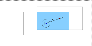
Figure 1: (color online) Representation of the integration procedure utilized in the evaluation of $Z_{2}$. The drawn points indicate particles 1 and 2. The solid line draw cavity-1 and -2, while the overlap region with volume $W$ is shaded. Dashed line plots the ES and EB.

II.1 CI of 2-HS in a cuboid pore

The empty cavity is characterized by the length parameters $L^{\prime}_{x}$, $L^{\prime}_{y}$, and $L^{\prime}_{z}$. We introduce the effective cavity length parameters $L_{i}=L^{\prime}_{i}-\sigma$, which characterize the available space for the center of one particle and the dimensionless lengths $l_{i}=L_{i}/\sigma$ with $i=x,\,y,\,z$. Then we obtain for the cuboid shaped pore $Z_{1}=L_{x}L_{y}L_{z}$, and

$$W(\mathbf{r})=\left|L_{x}-x\right|\left|L_{y}-y\right|\left|L_{z}-z\right|\;,$$ (7)

where $\mathbf{r}=(x,y,z)$ (see Fig. 1). The EB is a cuboid with doubled length sides and the $W(\mathbf{r})$ dependence turns convenient to integrate Eq. (6) over $0\leq x\leq L_{x}$, $0\leq y\leq L_{y}$, $0\leq z\leq L_{z}$ and multiply by $8$. Although, $W(\mathbf{r})$ is positive defined for any $\mathbf{r}$ and it is a non analytic function. For practical purposes we will extend analytically $W$ to enlarge the integration domain outside the EB box to $x\geq 0$, $y\geq 0$, and $z\geq 0$. Assuming $L_{x}\leq L_{y}\leq L_{z}$ it is necessary to analyze the integral (6) for different pore size domains in the parameter space $\mathbf{X}=(L_{x},L_{y},L_{z})$ or the similar $\mathbf{X}=(l_{x},l_{y},l_{z})$. Introducing the directions: $\hat{xy}\propto L_{x}\hat{x}+L_{y}\hat{y}$, $\hat{xz}\propto L_{x}\hat{x}+L_{z}\hat{z}$, $\hat{yz}\propto L_{y}\hat{y}+L_{z}\hat{z}$, and $\hat{xyz}\propto L_{x}\hat{x}+L_{y}\hat{y}+L_{z}\hat{z}$ we may distinguish eight different regions of $\mathbf{X}$.

Region 1

The large pore domain is defined by the condition that ES is completely enclosed into the EB, i.e., that $l_{i}\geq 1$ with $i=x,\,y,\,z$. The integral (6) splits into the simpler ones,

$$\mathcal{I}_{1}=8\int_{0}^{L_{x}}dx\,\int_{0}^{L_{y}}dy\,\int_{0}^{L_{z}}\,W\,dz=Z_{1}^{2}\;,$$ (8)

$$\mathcal{I}_{2} = 8\int_{0}^{\sigma}dx\,\int_{0}^{\sqrt{\sigma^{2}-x^{2}}}dy\,\int_{0}^{\sqrt{\sigma^{2}-x^{2}-y^{2}}}\,W\,dz\;,$$ (9)

$$= \frac{4\pi}{3}\sigma^{3}L_{x}L_{y}L_{z}-\frac{\pi}{2}\sigma^{4}(L_{x}L_{y}+L_{x}L_{z}+L_{y}L_{z})+$$

$$\frac{8}{15}\sigma^{5}(L_{x}+L_{y}+L_{z})-\frac{1}{6}\sigma^{6}\;,$$

which in terms of dimensionless length variables is

$$\mathcal{I}_{2} = \frac{4\pi}{3}\sigma^{6}l_{x}l_{y}l_{z}-\frac{\pi}{2}\sigma^{6}(l_{x}l_{y}+l_{x}l_{z}+l_{y}l_{z})+$$ (10)

$$\frac{8}{15}\sigma^{6}(l_{x}+l_{y}+l_{z})-\frac{1}{6}\sigma^{6}\;.$$

Then, we find

$$Z_{2}=\mathcal{I}_{1}-\mathcal{I}_{2}=Z_{1}^{2}-2\,Z_{1}b_{2}(cub)\;.$$ (11)

Last expression is similar to Eq. (5).

Region 2

The ES exceeds only two faces of the EB domain. Here, the exclusion sphere showed in Fig. 1 should extend beyond the EB at most in one direction normal to the faces of the box. As far as this direction was labeled as $\hat{x}$, then we have $l_{x}\leq 1$, $l_{y}\geq 1$, and $l_{z}\geq 1$. We define the auxiliary integral $\mathcal{I}_{3x}$, its integration domain is the spherical cup outside the EB box in the $\hat{x}$ direction

$$\mathcal{I}_{3x} = 8\int_{L_{x}}^{\sigma}dx\,\int_{0}^{\sqrt{\sigma^{2}-x^{2}}}dy\,\int_{0}^{\sqrt{\sigma^{2}-x^{2}-y^{2}}}\,W\,dz\;,$$ (12)

$$= \sigma^{6}\left\{-\frac{1}{30}\left(1-l_{x}\right)^{4}\left(5+4l_{x}+l_{x}^{2}\right)-\frac{\pi}{6}\,l_{y}l_{z}\left(1-l_{x}\right)^{3}\left(l_{x}+3\right)+\right.\;,$$

$$\left.\left(l_{y}+l_{z}\right)\left[\frac{1}{15}\,\sqrt{1-l_{x}^{2}}\,\left(8+9\,l_{x}^{2}-2\,l_{x}^{4}\right)-l_{x}\left(\frac{\pi}{2}-\arcsin(l_{x})\right)\right]\right\}$$

$$Z_{2}=\mathcal{I}_{1}-\mathcal{I}_{2}+\mathcal{I}_{3x}\;,$$ (13)

In the same sense, we define $\mathcal{I}_{3i}$ with $i=x,y,z$. The integration domain of $\mathcal{I}_{3i}$ corresponds to the spherical cup outside the EB in the $\hat{i}$ direction, which completes the description of the set of functions $\{\mathcal{I}_{3x},\,\mathcal{I}_{3y},\,\mathcal{I}_{3z}\}$.

Region 3

We consider the situation when ES exceeds only four faces of the EB, where the exclusion sphere must extend beyond the cuboidal EB in $\hat{x}$ and $\hat{y}$ directions but not in directions $\hat{z}$ and $\hat{xy}$. In this case $l_{x}\leq 1$, $l_{y}\leq 1$, $l_{z}\geq 1$ and $l_{x}^{2}+l_{y}^{2}\geq 1$. The CI is

$$Z_{2}=\mathcal{I}_{1}-\mathcal{I}_{2}+\mathcal{I}_{3x}+\mathcal{I}_{3y}\;.$$ (14)

Region 4

The next domain to consider is when ES exceeds all six faces of EB but any more. It goes beyond the EB in $\{\hat{x},\hat{y},\hat{z}\}$ directions but not in $\{\hat{xy},\hat{xz},\hat{yz}\}$. Then, we need $l_{i}\leq 1$ and $l_{i}^{2}+l_{j}^{2}\geq 1$, for $i,j=x,\,y,\,z$ with $i\neq j$, therefore

$$Z_{2}=\mathcal{I}_{1}-\mathcal{I}_{2}+\mathcal{I}_{3x}+\mathcal{I}_{3y}+\mathcal{I}_{3z}\;.$$ (15)

Region 5

In this region ES exceeds at four faces and four edges of EB. The sphere fall off the EB in $\{\hat{x},\hat{y},\hat{xy}\}$ directions but not in $\hat{z}$. Then we have obtain $l_{x}^{2}+l_{y}^{2}\leq 1$ and $l_{z}\geq 1$. We define the auxiliary integral $\mathcal{I}_{3xy}$, its integration domain is the right angle spherical wedge outside the EB in both $\hat{x}$ and $\hat{y}$ directions. Note that the edge of the spherical wedge does not cross the sphere center. In addition, we define $\mathcal{I}_{2xy}$ , its integration domain is the space outer to ES and inner to EB,

$$\mathcal{I}_{3xy}=8\int_{L_{x}}^{\sqrt{\sigma^{2}-L_{y}^{2}}}dx\,\int_{L_{y}}^{\sqrt{\sigma^{2}-x^{2}}}dy\,\int_{0}^{\sqrt{\sigma^{2}-x^{2}-y^{2}}}\,W\,dz\;,$$ (16)

$$\mathcal{I}_{2xy} = 8\int_{0}^{L_{x}}dx\,\int_{0}^{L_{y}}dy\,\int_{0}^{\sqrt{\sigma^{2}-x^{2}-y^{2}}}\,W\,dz\;,$$ (17)

both integrals are related by

$$\mathcal{I}_{2xy}=\mathcal{I}_{2}-\mathcal{I}_{3x}-\mathcal{I}_{3y}+\mathcal{I}_{3xy}\;.$$ (18)

For $\mathcal{I}_{2xy}$ we found

$$\mathcal{I}_{2xy} = \sigma^{6}\left\{-\frac{1}{6}l_{x}^{2}l_{y}^{2}\left(6-l_{x}^{2}-l_{y}^{2}\right)+\frac{8}{15}l_{z}+\right.\;,$$ (19)

$$\left.\frac{1}{15}l_{z}\,\sqrt{1-l_{x}^{2}-l_{y}^{2}}\,\left[8+9\,(l_{x}^{2}+l_{y}^{2})-2\,(l_{x}^{4}+l_{y}^{4})+6l_{x}^{2}l_{y}^{2}\right]-\right.$$

$$\left.\frac{8}{3}l_{x}l_{y}l_{z}\arctan\left(\frac{l_{x}l_{y}}{\sqrt{1-l_{x}^{2}-l_{y}^{2}}}\right)+l_{z}\left[\mathcal{H}(l_{x},l_{y})+\mathcal{H}(l_{y},l_{x})\right]\right\}\>,$$

$$\mathcal{H}(u,v)=-\frac{1}{15}\,\sqrt{1-u^{2}}\,\left(8+9\,u^{2}-2\,u^{4}\right)-u\,\arcsin(u)+\frac{1}{3}v\left(3+6\,u^{2}-u^{4}\right)\arcsin\left(\frac{v}{\sqrt{1-u^{2}}}\right)\>.$$ (20)

The straight forward generalization of $\mathcal{I}_{2xy}$ and $\mathcal{I}_{3xy}$ in Eqs. (16, 17) defines the set of functions $\{\mathcal{I}_{2xy},\,\mathcal{I}_{2xz},\,\mathcal{I}_{2yz},$ $\,\mathcal{I}_{3xy},\,\mathcal{I}_{3xz},\,\mathcal{I}_{3yz}\}$. The zone of the phase space with non-null integrand in Eq. (1), i.e. the available phase space of the system (APS) breaks or fragments in two equal unlinked zones because the pair of particles can not interchange its positions anymore. In this sense we refer to an ergodicity breaking in the canonical ensemble, which introduce an overall factor $\xi=1/2$ in the CI, therefore

$$Z_{2}=\xi*\left(\mathcal{I}_{1}-\mathcal{I}_{2xy}\right)\;.$$ (21)

Note that $\xi$ was not explicitly written in Eq. (5) and then a $\xi=1$ value was there assumed.

Region 6

In this region ES exceeds at six faces and only four edges of EB. Here, the sphere should exceeds the EB in $\{\hat{x},\hat{y},\hat{z},\hat{xy}\}$ directions but not in $\{\hat{xz},\hat{yz}\}$. Then, the region in the parameter space is $l_{x}^{2}+l_{y}^{2}\leq 1$, $l_{z}\leq 1$, $l_{x}^{2}+l_{z}^{2}\geq 1$, and $l_{y}^{2}+l_{z}^{2}\geq 1$. For this region the particles can not interchange its positions, thus, the APS breaks into two equal and unlinked zones. The ergodicity breaking introduce the overall factor $\xi=1/2$,

$$Z_{2}=\xi*\left(\mathcal{I}_{1}-\mathcal{I}_{2xy}+\mathcal{I}_{3z}\right)\;.$$ (22)

Region 7

When ES exceeds at six faces and only eight edges but any vertex of EB we have the seventh region. Here, the sphere exceeds the EB in $\{\hat{x},\hat{y},\hat{z},\hat{xy},\hat{xz}\}$ directions but not in $\hat{yz}$. The parameter domain is $l_{z}\leq 1$, $l_{x}^{2}+l_{y}^{2}\leq 1$, $l_{x}^{2}+l_{z}^{2}\leq 1$, and $l_{y}^{2}+l_{z}^{2}\geq 1$. Again, APS breaks but now into four equal and unlinked zones each one characterizing a set of microestates, which is non-symmetric under some of the symmetries of the cuboid cavity. This is a spontaneous symmetry breaking phenomena. The ergodicity breaking produces a factor $\xi=1/4$, and the CI reads

$$Z_{2} = \xi*\left(\mathcal{I}_{1}-\mathcal{I}_{2}+\mathcal{I}_{3x}+\mathcal{I}_{3y}+\mathcal{I}_{3z}-\mathcal{I}_{3xy}-\mathcal{I}_{3xz}\right)\;,$$ (23)

$$= \xi*\left(\mathcal{I}_{1}-\mathcal{I}_{2xy}+\mathcal{I}_{3z}-\mathcal{I}_{3xz}\right)\;.$$

Region 8

The last region considered is when ES exceeds at six faces, twelve edges but any vertex of EB. Then, the sphere exceeds the EB box in $\{\hat{x},\hat{y},\hat{z},\hat{xy},\hat{xz},\hat{yz}\}$ direction but not in $\hat{xyz}$. Then, $l_{i}^{2}+l_{j}^{2}\leq 1$ for $i,j=x,\,y,\,z$ ($i\neq j$), and $l_{x}^{2}+l_{y}^{2}+l_{z}^{2}\geq 1$. With this conditions the APS breaks into eight equal and unlinked zones which also involves a spontaneous symmetry breaking. The factor introduced by the ergodicity breaking is $\xi=1/8$, while CI is

$$Z_{2}=\xi*\left(\mathcal{I}_{1}-\mathcal{I}_{2}+\mathcal{I}_{3x}+\mathcal{I}_{3y}+\mathcal{I}_{3z}-\mathcal{I}_{3xy}-\mathcal{I}_{3xz}-\mathcal{I}_{3yz}\right)\;.$$ (24)

Finally, in the case that ES exceeds the EB also in $\hat{xyz}$ direction, the partition function becomes null because both particles do not fit into the cavity.

II.2 CI of 2-HS in a cylindrical pore

Let us define the usual length parameters, height and radius, that characterize an empty cylindrical cavity $L_{h}^{\prime}$, $R^{\prime}$. The effective cavity length parameters are then $L_{h}=L_{h}^{\prime}-\sigma$, $R=R^{\prime}-\sigma/2$ and the dimensionless ones are given by $h=L_{h}/\sigma$, $\mathsf{R}=\mathsf{s}^{-1}=2R/\sigma$. For the cylindrical shaped pore we have $Z_{1}=\pi L_{h}\,R^{2}$. As it was above mentioned, we need to know the volume defined by the intersection of two equal and parallel cylinders, $W(\mathbf{r},L_{h},R)$. It is related to the intersection of two disks of equal radii $R$ and separated by a distance $r$, $W_{disk}(r,R)=2R^{2}\left[\arccos(\mathsf{r})-\mathsf{r}\left(1-\mathsf{r}^{2}\right)^{1/2}\right]$, where $\mathsf{r}=r/(2R)$ by

$$W(\mathbf{r},L_{h},R)=\left|L_{h}-z\right|W_{disk}(r,R)\;.$$ (25)

Note that $W$ is a well defined function of $\mathsf{r}$ only for the range $0<\mathsf{r}<1$. The EB is a cylinder of double lengths and the $W$ dependence turns convenient to integrate over $0\leq z\leq L_{h}$, $0\leq r\leq 2R$ and multiply by $4\pi$. The analytic extension of $W$ for values $z\geq 0$ will be considered when it becomes necessary. We need to analyze the integral considering the parameters $\mathbf{X}=(R,L_{h})$ which define the allowed pore size domain. Defining $\hat{rz}\propto R\,\hat{r}+(L_{h}/2)\,\hat{z}$ we distinguish four regions.

Region 1

The large pore domain is defined by the condition that the ES is completely enclosed into the EB, i.e., that $h\geq 1$ and $\mathsf{R}\geq 1$. The CI splits into,

$$\mathcal{I}_{1}=4\pi\int_{0}^{2R}r\,dr\,\int_{0}^{L_{h}}\,W\,dz=Z_{1}^{2}\;,$$ (26)

$$\mathcal{I}_{2} = 4\pi\int_{0}^{\sigma}r\,dr\,\int_{0}^{\sqrt{\sigma^{2}-r^{2}}}\,W\,dz\;,$$ (27)

$$= \pi^{2}R^{2}L_{h}\frac{4}{3}\sigma^{3}-\pi^{2}R^{2}\frac{1}{2}\sigma^{4}-\pi^{2}R\,L_{h}\frac{1}{2}\sigma^{4}\left[1-\,_{2}F_{1}(-\frac{1}{2},\frac{1}{2};3;\mathsf{s}^{2})\right]$$

$$+\frac{\pi}{12}\sigma\,\sqrt{(2R)^{2}-\sigma^{2}}(-6R^{4}+5R^{2}\sigma^{2}+\sigma^{4})$$

$$+\pi R^{2}(2R^{4}-2R^{2}\sigma^{2}+\sigma^{4})\arcsin(\mathsf{s})\;,$$

where ${}_{2}F_{1}(-\frac{1}{2},\frac{1}{2};3;a)$ is the Gauss hypergeometric function which can also be written in terms of complete elliptic integrals Abramowitz72 ; functionswolfram . The CI is then

$$Z_{2}=\mathcal{I}_{1}-\mathcal{I}_{2}\;.$$ (28)

Region 2

The ES exceeds only the bases of EB, domain. Here, the exclusion sphere should go beyond the EB only in the $\hat{z}$ direction and then $h\leq 1$, $\mathsf{R}\geq 1$. We define the auxiliary integral $\mathcal{I}_{3z}$, its integration domain is the spherical cup outside the upper base of the EB

$$\mathcal{I}_{3z} = 4\pi\int_{0}^{\sqrt{\sigma^{2}-L_{h}^{2}}}r\,dr\,\int_{L_{h}}^{\sqrt{\sigma^{2}-r^{2}}}\,W\,dz\;,$$ (29)

$$= R^{6}\pi/45\left\{-256h\mathsf{s}^{2}(-2+7\mathsf{s}^{2}+3\mathsf{s}^{4})\,E\left(\arcsin\left(\mathsf{s}\,\sqrt{1-h^{2}}\right),\mathsf{s}^{-2}\right)\right.$$

$$\left.+15\pi\,(3-12(1+h^{2})\mathsf{s}^{2}+64h\mathsf{s}^{4})-256h\mathsf{s}^{3}(1+2s^{2}-3\mathsf{s}^{4})\,F\left(\arccos\left(h\right),\mathsf{s}^{2}\right)\right.$$

$$\left.+2\mathsf{s}\,\sqrt{(1-h^{2})(1-(1-h^{2})\mathsf{s}^{2})}\left[-45+2(75+41h^{2})\mathsf{s}^{2}-24(-5-4h^{2}+h^{4})\mathsf{s}^{4}\right]\right.$$

$$\left.+30(-3+12(1+h^{2})\mathsf{s}^{2}+8(-3-6h^{2}+h^{4})\mathsf{s}^{4})\,\arccos\left(\mathsf{s}\,\sqrt{1-h^{2}}\right)\right\}\;,$$

where $F(a,b)$ and $E(a,b)$ are the incomplete elliptic integrals of the first and second kind respectively Abramowitz72 . The CI is

$$Z_{2}=\mathcal{I}_{1}-\mathcal{I}_{2}+\mathcal{I}_{3z}\;.$$ (30)

Region 3

In this case ES exceeds only the curved lateral face of EB. The exclusion sphere should go beyond the cylindrical EB only in the $\hat{r}$ direction being $h\geq 1$ and $\mathsf{R}\leq 1$. With these conditions particles can not interchange its positions producing that APS breaks into two equal and unlinked zones. We introduce the auxiliary integral $\mathcal{I}_{2r}$ is given by

$$\mathcal{I}_{2r} = 4\pi\int_{0}^{2R}r\,dr\,\int_{0}^{\sqrt{\sigma^{2}-r^{2}}}\,W\,dz\;,$$ (31)

$$= \pi^{2}\,(R^{6}-R^{4}\sigma^{2}+\frac{4}{3}R^{2}L_{h}\sigma^{3})+\frac{4\pi}{45}L_{h}\sigma\,\times$$

$$\left[(32R^{4}-28R^{2}\sigma^{2}-3\sigma^{4})\,E(\mathsf{s}^{-2})+(-16R^{4}-8R^{2}\sigma^{2}+3\sigma^{4})\,K(\mathsf{s}^{-2}))\right]\;,$$

where $K(a)$ and $E(a)$ are the complete elliptic integrals of the first and second kind, respectively. We may also formally define $\mathcal{I}_{3r}=\mathcal{I}_{2}-\mathcal{I}_{2r}$. The ergodicity breaking produces a $\xi=1/2$ factor, being $Z_{2}$

$$Z_{2}=\xi*\left(\mathcal{I}_{1}-\mathcal{I}_{2r}\right)=\xi*\left(\mathcal{I}_{1}-\mathcal{I}_{2}+\mathcal{I}_{3r}\right)\;.$$ (32)

Region 4

This region appears when ES exceeds both the bases and the curved lateral face but not the edges of EB. Therefore, the exclusion sphere exceeds EB in the $\{\hat{r},\hat{z}\}$ directions, but not in $\hat{rz}$. In consequence $h\leq 1$ and $\mathsf{R}\leq 1$, but $h^{2}+\mathsf{R}^{2}\geq 1$. As happens in Region 3, here the APS breaks into two equal and unlinked zones due to the ergodicity breaking, being $\xi=1/2$ and

$$Z_{2}=\xi*\left(\mathcal{I}_{1}-\mathcal{I}_{2}+\mathcal{I}_{3z}+\mathcal{I}_{3r}\right)\;.$$ (33)

Finally, if ES exceeds also in $\hat{rz}$ direction, the partition function becomes null because both particles can not fit into the pore.

II.3 CI of 2-HS in a spheroidal pore

The last CI that we evaluate in PW corresponds to the ellipsoidal pore. We restrict the study to cavities where only two principal radii are independent, i.e. to the revolution ellipsoids also called spheroids. Therefore, two distinct shapes the prolate and the oblate ones will be analyzed. Let us consider an effective cavity with spheroidal shape. The effective length parameters are the principal radii $R$ and $R_{c}$, where $R_{c}$ is the different radius. Dimensionless parameters are $\mathsf{R}=\mathsf{s}^{-1}=2R/\sigma$, $\mathsf{C}=2R_{c}/\sigma$, and $\lambda=R_{c}/R$. For $\lambda<1$ we deal with the oblate, while for $\lambda>1$ we deal with the prolate, spheroids. The configuration integral for one particle is $Z_{1}=\frac{4\pi}{3}\,R^{2}R_{c}$. The volume of intersection of two equally oriented spheroids, $W(r,z)$, is related with the volume of the intersection of two spheres. In terms of $W_{sphere}(\varrho,R)=\frac{4\pi}{3}\,R^{3}(1-\frac{3}{2}\mathsf{r}+\frac{1}{2}\mathsf{r}^{3})$ with $\varrho$ the spherical radial coordinate, and $\mathsf{r}=\varrho/(2R)$ we obtain

$$W(r,z)=\lambda W_{sphere}(\sqrt{r^{2}+(z/\lambda)^{2}},R)\;.$$ (34)

Function $W$ is well defined in the domain $0\leq r^{2}+(z/\lambda)^{2}\leq 4R^{2}$. The EB is a spheroid with double length radii. For this pore geometry none analytic extension is suitable and the $W$ dependence turns convenient to integrate over $0\leq z\leq 2R_{c}$, $0\leq r\leq 2R$, and multiply by $4\pi$. We need to analyze the integral considering the allowed values of parameters $\mathbf{X}=(R,R_{c})$ that define the pore size domain. We may distinguish three regions.

Region 1

In the large pore domain ES is completely enclosed into EB, i.e. $\mathsf{C}\geq 1$ and $\mathsf{R}\geq 1$. As it was above described, the integral splits into,

$$\mathcal{I}_{1}=4\pi\int_{0}^{2R_{c}}dz\,\int_{0}^{\sqrt{(2R)^{2}-z^{2}\lambda^{-2}}}\,W\,r\,dr=Z_{1}^{2}\;,$$ (35)

$$\mathcal{I}_{2} = 4\pi\int_{0}^{\sigma}dz\,\int_{0}^{\sqrt{\sigma^{2}-r^{2}}}\,W\,r\,dr\;,$$ (36)

$$= \frac{16}{9}\pi^{2}R^{3}\lambda\sigma^{3}-\frac{\pi^{2}\sigma^{4}}{2}\left(R^{2}-\frac{\sigma^{2}}{24}\right)\left(1+\frac{\lambda^{2}}{\sqrt{-1+\lambda^{2}}}\mathrm{arcsec}(\lambda)\right)+\frac{\pi^{2}}{72}\frac{\sigma^{6}}{\lambda^{2}}\;,$$

which concerns to both, oblated and prolated spheroidal cavities. For $\lambda<1$, $(-1+\lambda^{2})^{1/2}\mathrm{arcsec}(\lambda)$ transforms to $(1-\lambda^{2})^{1/2}\mathrm{arcsech}(\lambda)$. Although, for $\lambda\rightarrow 1$ we obtain $(-1+\lambda^{2})^{1/2}\mathrm{arcsec}(\lambda)\rightarrow 1$ which is consistent with the spherical pore result Urrutia_2008 . In terms of $\mathcal{I}_{1}$ and $\mathcal{I}_{2}$ we find

$$Z_{2}=\mathcal{I}_{1}-\mathcal{I}_{2}\;.$$ (37)

Next regions concern the situation where ES exceeds EB. Under such condition it becomes necessary to make a separate analysis of prolate and oblate, ellipsoids.

Region 2 (oblate)

Here we consider an oblate ellipsoid, $\lambda<1$. In this region ES exceeds on top and down directions of EB, i.e. in the direction of the principal axis $\hat{z}$, but not in $\hat{r}$. Therefore, we consider $\mathsf{C}\leq 1$, $\mathsf{R}>1$. We find that in this region it is simpler to deal directly with $Z_{2}$, we obtain

$$Z_{2} = 4\pi\int_{0}^{z_{max}}dz\,\int_{\sqrt{\sigma^{2}-z^{2}}}^{\sqrt{(2R)^{2}-z^{2}\lambda^{-2}}}\,W\,r\,dr\;,$$ (38)

$$= \frac{\sigma^{6}\lambda^{2}\pi^{2}}{144\,\sqrt{1-\lambda^{2}}}\left[-\mathsf{R}\,\sqrt{\mathsf{R}^{2}-1}\left(3+16\mathsf{R}^{2}-4\mathsf{R}^{4}\right)-3\left(6\mathsf{R}^{2}-1\right)\mathrm{arcsech}(\mathsf{R}^{2})\right]\;,$$

with $z_{max}=\lambda\sqrt{\frac{(2R)^{2}-\sigma^{2}}{1-\lambda^{2}}}$. We may also, formally define $\mathcal{I}_{2z}=\mathcal{I}_{1}-Z_{2}$ and $\mathcal{I}_{3z}=\mathcal{I}_{2}-\mathcal{I}_{2z}$. In the case that ES also exceeds EB in the $\hat{r}$ direction the partition function becomes null because both particles can not fit into the pore.

Region 3 (prolate)

Here we restrict to a prolate ellipsoid, $\lambda>1$. In this region ES exceeds in the lateral direction the surface of EB. Then, ES goes beyond EB only in $\hat{r}$ direction, but not in $\hat{z}$, i.e. $\mathsf{C}>1$, $\mathsf{R}\leq 1$. Under these conditions APS breaks into two equal and unlinked zones and the ergodicity breaking produce the factor $\xi=1/2$. Again, in this region is preferable to deal directly with $Z_{2}$

$$Z_{2}=\xi*4\pi\int_{0}^{r_{max}}r\,dr\,\int_{\sqrt{\sigma^{2}-r^{2}}}^{\lambda\,\sqrt{(2R)^{2}-r^{2}}}\,W\,dz\;,$$ (39)

where $r_{max}=\sqrt{\sigma^{2}-(\lambda 2R)^{2}}/\sqrt{\lambda^{2}-1}$. This integral was solved by splitting it in several parts, after some work we obtain

$$Z_{2}\xi^{-1} = \mathcal{I}_{1}-\frac{16}{9}\pi^{2}R^{3}\lambda\sigma^{3}+\frac{\pi^{2}\sigma^{4}}{2}R^{2}-\frac{\pi^{2}\sigma^{6}}{24}\left(\frac{1}{2}+\frac{1}{3\lambda^{2}}\right)$$ (40)

$$+\frac{\pi^{2}\sigma^{6}\lambda^{2}}{144\sqrt{-1+\lambda^{2}}}\,\mathsf{R}\,\sqrt{1-\mathsf{R}^{2}}\left(3+16\mathsf{R}^{2}-4\mathsf{R}^{4}\right)$$

$$+\frac{3\sigma^{6}\lambda^{2}\pi^{2}}{144\,\sqrt{-1+\lambda^{2}}}\left(6\mathsf{R}^{2}-1\right)\left[\mathrm{arcsec}(\lambda)-\arccos(\mathsf{R})\right]\>,$$

Formally, we can define $\mathcal{I}_{2r}=\mathcal{I}_{1}-\xi^{-1}Z_{2}$ and $\mathcal{I}_{3r}$=$\mathcal{I}_{2}$-$\mathcal{I}_{2r}$. In addition, we note that if the exclusion sphere exceeds EB all around, particles do not fit into the cavity and then the CI becomes null. The Eq. (40) is the last result about analytic expressions for the CI of 2-HS system confined in the studied cuboid, cylindrical and spheroidal, cavities.

In PW we deal with a pair of distinguishable particles. Even sow, we make a brief discussion about the CI of a system of two indistinguishable HS (2i-HS). The canonical partition function of 2i-HS confined in a cuboidal, cylindrical, spheroidal and other shaped cavities are easily obtained from the CI of a 2-distinguishable-HS with the introduction of minor modifications. The first obvious change comes in the partition function definition because we must introduce the correct Boltzmann factor then $Q_{2,ind}=\frac{1}{2}\Lambda^{-6}Z_{2,ind}$. Secondly, we must analize the difference between $Z_{2}$ and $Z_{2,ind}$. In principle, expression (1) gives the starting point to define both, $Z_{2}$ and $Z_{2,ind}$. However, the evaluation of $Z_{2}$ for the studied cavities involves the factor $\xi$ that modifies Eq. (1) in some regions. We recognize that $Z_{2,ind}=Z_{2}$ in regions where no extra factor appears. A detailed inspection of the origin of $\xi$ also shows other different situations. In some regions the ergodicity breaking appears because particles can not interchange their positions, but this makes non sense for indistinguishable particles. Therefore, regions where $\xi=1/2$ corresponds to $\xi_{ind}=1$. In other regions the ergodicity breaking also involves the spontaneous symmetry breaking, in this regions we find $\xi_{ind}=2\xi$. In summary

$$Z_{2,ind}=\xi_{ind}\,Z_{2}(\xi=1)\>,\textrm{ with }\xi_{ind}=2\xi\textrm{ if }\xi\neq 1\>,$$

and $\xi_{ind}=2$ if $\xi=1$. Remarkably, partition function relates simply by $Q_{2,ind}=Q_{2}$ if $\xi\neq 1$, and $Q_{2,ind}=\frac{1}{2}Q_{2}$ if $\xi=1$.

III Local properties: Density distribution and Pressure

In principle, the partition function of the system holds in its global Statistical Mechanic properties. Such properties are presumably obtainable from some derivatives of $Q_{2}$. This makes interesting the study of the analytical properties of $Z_{2}$ which is done in Sec. IV. Now, we are also interested in the local properties of the 2-HS confined system. Therefore, we study two functions, the one body density distribution $\rho(\mathbf{r})$ and the pressure tensor $\mathbf{P}(\mathbf{r})$. We begin with a general brief description of the properties of $\rho(\mathbf{r})$. For any pore shape, $\rho(\mathbf{r})$ is (Hill56, , p.180)

$$\rho(\mathbf{r}) = 2Z_{2}^{-1}e_{1}(\mathbf{r})\,\int\,e_{2}(\mathbf{r}_{2})\,e_{12}(\left|\mathbf{r}-\mathbf{r}_{2}\right|)\,d\mathbf{r}_{2}\>,$$ (41)

$$= 2Z_{2}^{-1}\,e_{1}(\mathbf{r})\,\left(Z_{1}-\mathcal{J}_{2}(\mathbf{r})\right)\>,$$

$$\mathcal{J}_{2}(\mathbf{r})=-\int\,e_{2}(\mathbf{r}_{2})\,f_{12}(\left|\mathbf{r}-\mathbf{r}_{2}\right|)\,d\mathbf{r}_{2}\>,$$ (42)

where $\mathcal{J}_{2}(\mathbf{r})$ is the overlap volume between the cavity and the ES (with $\sigma$ radius) at position $\mathbf{r}$. This ES is produced by one HS-particle located there. The complete integral is $\int\rho(\mathbf{r})\,d\mathbf{r}=2$. For an arbitrary $\mathbf{r}$, $\mathcal{J}_{2}(\mathbf{r})$ is positive and continuous but non-analytical and may be piecewise defined. When the particle is placed sufficiently deep inside the cavity all the ES is inner to the boundary. Therefore, for $\mathbf{r}$ such that the shortest distance to the boundary is greater than $\sigma$, $\mathcal{J}_{2}(\mathbf{r})$ reaches its maximum value $\mathcal{J}_{2}(\mathbf{r})=2b_{2}$. This means that for big enough cavities of any shape a plateau of constant density

$$\rho_{0}=2Z_{2}^{-1}\left(Z_{1}-2b_{2}\right)\>,$$ (43)

develops at a distance to the boundary grater than $\sigma$. When $\mathbf{r}$ becomes nearer to the boundary the function $\mathcal{J}_{2}(\mathbf{r})$ decreases and $\rho(\mathbf{r})$ increases. For $\mathbf{r}$ outside of the cavity $\rho(\mathbf{r})=0$, but we can define its continuous extension $y(\mathbf{r})$ by dropping out the $e_{1}(\mathbf{r})$ term in Eqs. (41). Outside of the cavity, for distances to the boundary greater than $\sigma$, $y(\mathbf{r})$ becomes constant because $\mathcal{J}_{2}(\mathbf{r})=0$. The $\mathcal{J}_{2}(\mathbf{r})$ for the cuboid and cylindrical pores may be expressed by combining the $2b_{2}$ constant and the geometrical functions $\{\mathcal{J}_{2a}(\mathbf{r}\cdot\hat{\mathbf{a}}),\,\mathcal{J}_{2ab}(\mathbf{r}\cdot\hat{\mathbf{a}},\mathbf{r}\cdot\hat{\mathbf{b}}),\,\mathcal{J}_{2abc}(\mathbf{r}\cdot\hat{\mathbf{a}},\mathbf{r}\cdot\hat{\mathbf{b}},\mathbf{r}\cdot\hat{\mathbf{c}})\}$, where $\{a,b,c\}$ represent characteristic directions normal to the cavity boundary with inward normal versors $\{\hat{\mathbf{a}},\hat{\mathbf{b}},\hat{\mathbf{c}}\}$. The function $\mathcal{J}_{2a}$ is the inner overlap volume defined by the ES and one boundary surface that intersects it, $\mathcal{J}_{2ab}$ is the inner overlap volume defined by the sphere and two intersecting boundary surfaces, and $\mathcal{J}_{2abc}$ involves three mutually intersecting boundary surfaces. The short cut $\mathbf{r}\cdot\hat{\mathbf{a}}$ and similar are the (minimum) distance between the ES center and a face of the boundary with normal inward versor $\hat{\mathbf{a}}$. Although, $\mathbf{r}\cdot\hat{\mathbf{a}}$ extends to negative values when $\mathbf{r}$ is outside of the cavity. We may mention that inner overlap volume clearly identify a unique volume and then this description is non-ambiguous. When position $\mathbf{r}$ is on a cavity surface with simple curvature and away from other surfaces (a distance greater than $\sigma$) $\mathcal{J}_{2}(\mathbf{r})=\mathcal{J}_{2a}(\mathbf{r}\cdot\hat{\mathbf{a}}=0)$ which reduces to simple expressions. In such conditions, we have $\mathcal{J}_{2}(0)=b_{2}$ for the planar surface, $\mathcal{J}_{2,sph}(0)=b_{2}(1-\frac{3}{4}\mathsf{s})$ for a concave spherical surface and $\mathcal{J}_{2,sph}(0)=b_{2}(1+\frac{3}{4}\mathsf{s})$ for the convex one Urrutia_2008 ; Urrutia_2010 . For $\mathbf{r}$ on the lateral curved surface of a cylinder the analytic expression involving elliptic integrals is known Lamarche_1990 . Its power series is, $\mathcal{J}_{2,cyl}(0)=b_{2}(1-\frac{3}{8}\mathsf{s}-\frac{1}{32}\mathsf{s}^{3})+O(\mathsf{s}^{5})$ and $\mathcal{J}_{2,cyl}(0)=b_{2}(1+\frac{3}{8}\mathsf{s}+\frac{1}{32}\mathsf{s}^{3})+O(\mathsf{s}^{5})$ for the concave and convex cases, respectively. The question becomes even worse for the spheroidal pore surface, where we found analytic expressions of $\mathcal{J}_{2,sphd}(0)$ only for points on the poles and on the equatorial line.

III.1 Density distribution in the cuboidal pore

For the cuboid cavity the boundary surfaces are orthogonally intersecting planes. Therefore, in cuboidal cavities, $\mathcal{J}_{2a}$ is the inner overlap volume defined by the ES and a plane that intersects it, $\mathcal{J}_{2ab}$ is the volume defined by the sphere and a right angle dihedron that intersects it, and $\mathcal{J}_{2abc}$ is the volume defined by the sphere and a right angle vertex. We must include a brief digression about the volume of intersection of a unit sphere and a set of mutually intersecting planes. As we are primarily interested in the cuboid we restrict ourselves to sets of mutually orthogonal planes with at most three planes. We introduce the function $\mathcal{K}_{a}(\mathbf{r}\cdot\hat{\mathbf{a}})$ which measures the volume of the spherical segment or spherical cap, defined by the intersection of the unit sphere at position $\mathbf{r}$ and a half-space with inward normal $\hat{\mathbf{a}}$. The vector $\mathbf{r}$ goes from a point in the plane to the sphere center. For $\hat{\mathbf{a}}=\hat{\mathbf{x}}$ we have $\mathbf{r}\cdot\hat{\mathbf{a}}=x$ with $x>0$ if the center of the sphere is in the positive half-space. For $-1\leq x\leq 0$,

$$\mathcal{K}_{x}(x) = 4\int_{-x}^{1}dx^{\prime}\,\int_{0}^{\sqrt{1-x^{\prime 2}}}dy^{\prime}\,\int_{0}^{\sqrt{1-y^{\prime 2}-x^{\prime 2}}}\,dz^{\prime}\;,$$ (44)

$$= \frac{\pi}{3}(1+x)^{2}(2-x)\;,$$ (45)

but Eq. (45) is also valid in the extended domain $-1\leq x\leq 1$. Naturally,

$$4\pi/3=\mathcal{K}_{a}(\mathbf{r}\cdot\hat{\mathbf{a}})+\mathcal{K}_{a}(-\mathbf{r}\cdot\hat{\mathbf{a}})\>,$$ (46)

$$\mathcal{K}_{a}(-\mathbf{r}\cdot\hat{\mathbf{a}})=\mathcal{K}_{\bar{a}}(-\mathbf{r}\cdot\hat{\mathbf{a}})\>,$$ (47)

where the label $\bar{a}=-a$ corresponds to the inward direction $-\hat{\mathbf{a}}$. The function $\mathcal{K}_{ab}(\mathbf{r}\cdot\hat{\mathbf{a}},\mathbf{r}\cdot\hat{\mathbf{b}})$ is the volume between the sphere and a right angle wedge when the edge cross the sphere. The wedge is defined by the quadrant determined by the intersection of half-spaces with inward directions $\hat{\mathbf{a}}$ and $\hat{\mathbf{b}}$. As far as the center of the sphere does not lie on the edge this spherical wedge is different to the usual one. For $\hat{\mathbf{a}}=\hat{\mathbf{x}}$ and $\hat{\mathbf{b}}=\hat{\mathbf{y}}$ we obtain

$$\mathcal{K}_{xy}(x,y) = 2\int_{x}^{\sqrt{1-y^{2}}}dx^{\prime}\,\int_{y}^{\sqrt{1-x^{\prime 2}}}dy^{\prime}\,\int_{0}^{\sqrt{1-y^{\prime 2}-x^{\prime 2}}}\,dz^{\prime}\;,$$ (49)

$$= \frac{1}{3}\left[\pi+2\,x\,y\,\sqrt{1-x^{2}-y^{2}}-2\,\arctan(\frac{x\,y}{\sqrt{1-x^{2}-y^{2}}})\right.$$

$$\left.+x\,(3-x^{2})\,\arccos(\frac{-y}{\sqrt{1-x^{2}}})+y\,(3-y^{2})\,\arccos(\frac{-x}{\sqrt{1-y^{2}}})\right]\;,$$

where Eq. (49) applies for $-1\leq x,y\leq 0$, $x^{2}+y^{2}<1$ but Eq. (49) is valid in the extended domain $-1\leq x,y\leq 1$, $x^{2}+y^{2}<1$. The half-length of the portion of the wedges edge inside the sphere is $1-x^{2}-y^{2}$. The function $\mathcal{K}_{ab}(\mathbf{r}\cdot\hat{\mathbf{a}},\mathbf{r}\cdot\hat{\mathbf{b}})$ has the following properties

$$\mathcal{K}_{a}(\mathbf{r}\cdot\hat{\mathbf{a}}) = \mathcal{K}_{ab}(\mathbf{r}\cdot\hat{\mathbf{a}},\mathbf{r}\cdot\hat{\mathbf{b}})+\mathcal{K}_{ab}(\mathbf{r}\cdot\hat{\mathbf{a}},-\mathbf{r}\cdot\hat{\mathbf{b}})\>,$$

$$\mathcal{K}_{b}(\mathbf{r}\cdot\hat{\mathbf{b}}) = \mathcal{K}_{ab}(\mathbf{r}\cdot\hat{\mathbf{a}},\mathbf{r}\cdot\hat{\mathbf{b}})+\mathcal{K}_{ab}(-\mathbf{r}\cdot\hat{\mathbf{a}},\mathbf{r}\cdot\hat{\mathbf{b}})\>,$$ (50)

$$4\pi/3=\mathcal{K}_{ab}(\mathbf{r}\cdot\hat{\mathbf{a}},\mathbf{r}\cdot\hat{\mathbf{b}})+\mathcal{K}_{ab}(-\mathbf{r}\cdot\hat{\mathbf{a}},\mathbf{r}\cdot\hat{\mathbf{b}})+\mathcal{K}_{ab}(\mathbf{r}\cdot\hat{\mathbf{a}},-\mathbf{r}\cdot\hat{\mathbf{b}})+\mathcal{K}_{ab}(-\mathbf{r}\cdot\hat{\mathbf{a}},-\mathbf{r}\cdot\hat{\mathbf{b}})\>,$$ (51)

$$\mathcal{K}_{ab}(\mathbf{r}\cdot\hat{\mathbf{a}},-\mathbf{r}\cdot\hat{\mathbf{b}}) = \mathcal{K}_{a\bar{b}}(\mathbf{r}\cdot\hat{\mathbf{a}},-\mathbf{r}\cdot\hat{\mathbf{b}})\>,$$

$$\mathcal{K}_{ab}(-\mathbf{r}\cdot\hat{\mathbf{a}},\mathbf{r}\cdot\hat{\mathbf{b}}) = \mathcal{K}_{\bar{a}b}(-\mathbf{r}\cdot\hat{\mathbf{a}},\mathbf{r}\cdot\hat{\mathbf{b}})\>,$$

$$\mathcal{K}_{ab}(-\mathbf{r}\cdot\hat{\mathbf{a}},-\mathbf{r}\cdot\hat{\mathbf{b}}) = \mathcal{K}_{\bar{a}\bar{b}}(-\mathbf{r}\cdot\hat{\mathbf{a}},-\mathbf{r}\cdot\hat{\mathbf{b}})\>,$$ (52)

being the Eq. (51) a consequence of Eqs. (46, 50). The last $\mathcal{K}$ function in which we are interested is $\mathcal{K}_{abc}(\mathbf{r}\cdot\hat{\mathbf{a}},\mathbf{r}\cdot\hat{\mathbf{b}},\mathbf{r}\cdot\hat{\mathbf{c}})$, the volume defined by the sphere and a right angle vertex inner to the sphere,

$$\mathcal{K}_{xyz}(x,y,z) = \int_{x}^{\sqrt{1-y^{\prime 2}-z^{\prime 2}}}dx^{\prime}\,\int_{y}^{\sqrt{1-x^{\prime 2}-z^{2}}}dy^{\prime}\,\int_{z}^{\sqrt{1-x^{\prime 2}-y^{\prime 2}}}\,dz^{\prime}\;,$$ (54)

$$= \frac{\pi}{6}+x\,y\,z-\frac{1}{4}\left[\mathcal{K}_{x}(x)+\mathcal{K}_{y}(y)+\mathcal{K}_{z}(z)\right]\;,$$

$$+\frac{1}{2}\left[\mathcal{K}_{xy}(x,y)+\mathcal{K}_{xz}(x,z)+\mathcal{K}_{yz}(y,z)\right]\;.$$

As happened before, Eq. (54) apply for $-1\leq x,y,z\leq 0$, $x^{2}+y^{2}+z^{2}<1$ but Eq. (54) is valid in the extended domain $-1\leq x,y,z\leq 1$, $x^{2}+y^{2}+z^{2}<1$. Interestingly, we were unable to perform the direct integration expressed in Eq. (54), although it was evaluated making a geometrical decomposition into simple terms. We obtain the following properties for $\mathcal{K}_{abc}(\mathbf{r}\cdot\hat{\mathbf{a}},\mathbf{r}\cdot\hat{\mathbf{b}},\mathbf{r}\cdot\hat{\mathbf{c}})$

$$\mathcal{K}_{ab}(\mathbf{r}\cdot\hat{\mathbf{a}},\mathbf{r}\cdot\hat{\mathbf{b}}) = \mathcal{K}_{abc}(\mathbf{r}\cdot\hat{\mathbf{a}},\mathbf{r}\cdot\hat{\mathbf{b}},\mathbf{r}\cdot\hat{\mathbf{c}})+\mathcal{K}_{abc}(\mathbf{r}\cdot\hat{\mathbf{a}},\mathbf{r}\cdot\hat{\mathbf{b}},-\mathbf{r}\cdot\hat{\mathbf{c}})\>,$$

$$\mathcal{K}_{ac}(\mathbf{r}\cdot\hat{\mathbf{a}},\mathbf{r}\cdot\hat{\mathbf{c}}) = \mathcal{K}_{abc}(\mathbf{r}\cdot\hat{\mathbf{a}},\mathbf{r}\cdot\hat{\mathbf{b}},\mathbf{r}\cdot\hat{\mathbf{c}})+\mathcal{K}_{abc}(\mathbf{r}\cdot\hat{\mathbf{a}},-\mathbf{r}\cdot\hat{\mathbf{b}},\mathbf{r}\cdot\hat{\mathbf{c}})\>,$$

$$\mathcal{K}_{bc}(\mathbf{r}\cdot\hat{\mathbf{b}},\mathbf{r}\cdot\hat{\mathbf{c}}) = \mathcal{K}_{abc}(\mathbf{r}\cdot\hat{\mathbf{a}},\mathbf{r}\cdot\hat{\mathbf{b}},\mathbf{r}\cdot\hat{\mathbf{c}})+\mathcal{K}_{abc}(-\mathbf{r}\cdot\hat{\mathbf{a}},\mathbf{r}\cdot\hat{\mathbf{b}},\mathbf{r}\cdot\hat{\mathbf{c}})\>,$$ (55)

$$4\pi/3 = \mathcal{K}_{abc}(\mathbf{r}\cdot\hat{\mathbf{a}},\mathbf{r}\cdot\hat{\mathbf{b}},\mathbf{r}\cdot\hat{\mathbf{c}})+\mathcal{K}_{abc}(-\mathbf{r}\cdot\hat{\mathbf{a}},-\mathbf{r}\cdot\hat{\mathbf{b}},-\mathbf{r}\cdot\hat{\mathbf{c}})+\mathcal{K}_{abc}(-\mathbf{r}\cdot\hat{\mathbf{a}},-\mathbf{r}\cdot\hat{\mathbf{b}},\mathbf{r}\cdot\hat{\mathbf{c}})\>,$$ (56)

$$+\mathcal{K}_{abc}(-\mathbf{r}\cdot\hat{\mathbf{a}},\mathbf{r}\cdot\hat{\mathbf{b}},-\mathbf{r}\cdot\hat{\mathbf{c}})+\mathcal{K}_{abc}(\mathbf{r}\cdot\hat{\mathbf{a}},-\mathbf{r}\cdot\hat{\mathbf{b}},-\mathbf{r}\cdot\hat{\mathbf{c}})\>,$$

$$+\mathcal{K}_{abc}(-\mathbf{r}\cdot\hat{\mathbf{a}},\mathbf{r}\cdot\hat{\mathbf{b}},\mathbf{r}\cdot\hat{\mathbf{c}})+\mathcal{K}_{abc}(\mathbf{r}\cdot\hat{\mathbf{a}},-\mathbf{r}\cdot\hat{\mathbf{b}},\mathbf{r}\cdot\hat{\mathbf{c}})+\mathcal{K}_{abc}(\mathbf{r}\cdot\hat{\mathbf{a}},\mathbf{r}\cdot\hat{\mathbf{b}},-\mathbf{r}\cdot\hat{\mathbf{c}})\>.$$

$$\mathcal{K}_{abc}(\mathbf{r}\cdot\hat{\mathbf{a}},\mathbf{r}\cdot\hat{\mathbf{b}},-\mathbf{r}\cdot\hat{\mathbf{c}}) = \mathcal{K}_{ab\bar{c}}(\mathbf{r}\cdot\hat{\mathbf{a}},\mathbf{r}\cdot\hat{\mathbf{b}},-\mathbf{r}\cdot\hat{\mathbf{c}})\>,$$

$$\mathcal{K}_{abc}(\mathbf{r}\cdot\hat{\mathbf{a}},-\mathbf{r}\cdot\hat{\mathbf{b}},-\mathbf{r}\cdot\hat{\mathbf{c}}) = \mathcal{K}_{a\bar{b}\bar{c}}(\mathbf{r}\cdot\hat{\mathbf{a}},-\mathbf{r}\cdot\hat{\mathbf{b}},-\mathbf{r}\cdot\hat{\mathbf{c}})\>,$$

$$\mathcal{K}_{abc}(-\mathbf{r}\cdot\hat{\mathbf{a}},-\mathbf{r}\cdot\hat{\mathbf{b}},-\mathbf{r}\cdot\hat{\mathbf{c}}) = \mathcal{K}_{\bar{a}\bar{b}\bar{c}}(-\mathbf{r}\cdot\hat{\mathbf{a}},-\mathbf{r}\cdot\hat{\mathbf{b}},-\mathbf{r}\cdot\hat{\mathbf{c}})\>,$$ (57)

where other identities similar to Eq. (57) may be obtained by symmetry considerations. To the best of our knowledge the basic geometrical functions $\mathcal{K}_{ab}$ and $\mathcal{K}_{abc}$ are new results never published before.

Using the $\mathcal{K}$ functions we can complete the picture of $\rho(\mathbf{r})$ for the cuboid cavity being that functions $\mathcal{J}_{2}$ and $\mathcal{K}$ are related by

$$\mathcal{J}_{2a}(\mathbf{r}\cdot\hat{\mathbf{a}}) = \sigma^{3}\mathcal{K}_{a}(\tilde{\mathbf{r}}\cdot\hat{\mathbf{a}})\>,$$

$$\mathcal{J}_{2ab}(\mathbf{r}\cdot\hat{\mathbf{a}},\mathbf{r}\cdot\hat{\mathbf{b}}) = \sigma^{3}\mathcal{K}_{ab}(\tilde{\mathbf{r}}\cdot\hat{\mathbf{a}},\tilde{\mathbf{r}}\cdot\hat{\mathbf{b}})\>,$$

$$\mathcal{J}_{2abc}(\mathbf{r}\cdot\hat{\mathbf{a}},\mathbf{r}\cdot\hat{\mathbf{b}},\mathbf{r}\cdot\hat{\mathbf{c}}) = \sigma^{3}\mathcal{K}_{abc}(\tilde{\mathbf{r}}\cdot\hat{\mathbf{a}},\tilde{\mathbf{r}}\cdot\hat{\mathbf{b}},\tilde{\mathbf{r}}\cdot\hat{\mathbf{c}})\>.$$ (58)

with $\tilde{\mathbf{r}}=\mathbf{r}/\sigma$. We take the three orthogonal planes at $x=0$, $y=0$, and $z=0$ with inward directions $\hat{\mathbf{x}}$, $\hat{\mathbf{y}}$, and $\hat{\mathbf{z}}$, respectively. Thus, $\{x,\,y,\,z\}$ represent the perpendicular distances to this set of planes. We assume a cuboidal pore such that $L_{i}>2\sigma$ (Region 1) and $0\leq x\leq y\leq z\leq 1$, therefore

$$\dfrac{\mathcal{J}_{2}(\mathbf{r})}{\sigma^{3}}= \begin{cases}2b_{2}\,,&x,y,z\geq 1\,,\\ \mathcal{K}_{x}(x)\,,&x<1,\,y\geq 1,\,z\geq 1\,,\\ 2b_{2}-\mathcal{K}_{x}(-x)-\mathcal{K}_{y}(-y)\,,&x,\,y<1,\,x^{2}+y^{2},\,z\geq 1\,,\\ 2b_{2}-\mathcal{K}_{x}(-x)-\mathcal{K}_{y}(-y)-\mathcal{K}_{z}(-z)\,,&x,\,y,\,z<1,\,x^{2}+y^{2},\,x^{2}+z^{2},\,y^{2}+z^{2}\geq 1\,,\\ \mathcal{K}_{xy}(x,y)\,,&x^{2}+y^{2}<1,\,z\geq 1\,,\\ \mathcal{K}_{xy}(x,y)-\mathcal{K}_{z}(-z)\,,&z,\,x^{2}+y^{2}<1,\,x^{2}+z^{2},\,y^{2}+z^{2}\geq 1\,,\\ \mathcal{K}_{x}(x)-\mathcal{K}_{xy}(x,-y)-\mathcal{K}_{xz}(x,-z)\,,&x^{2}+y^{2},\,x^{2}+z^{2}<1,\,y^{2}+z^{2}\geq 1\,,\\ \mathcal{K}_{y}(y)-\mathcal{K}_{xy}(-x,y)-\mathcal{K}_{yz}(y,-z)\,,&x^{2}+y^{2},\,y^{2}+z^{2}<1,\,x^{2}+z^{2}\geq 1\,,\\ \mathcal{K}_{x}(x)-\mathcal{K}_{xy}(x,-y)-\mathcal{K}_{xyz}(x,y,-z)\,,&x^{2}+y^{2},\,x^{2}+z^{2},\,y^{2}+z^{2}<1\,,x^{2}+y^{2}+z^{2}\geq 1\\ \mathcal{K}_{xyz}(x,y,z)\,,&x^{2}+y^{2}+z^{2}<1\>.\end{cases}$$ (59)

Following a similar procedure we can obtain $\mathcal{J}_{2}(\mathbf{r})$ for Regions from 2 to 8.

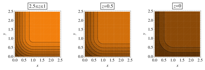
Figure 2: (Color online) Contour plot of the density distribution for a cubic pore with $L=5\sigma$. As gray becomes darker the density becomes higher.

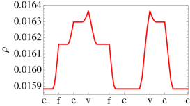
Figure 3: Density distribution for a closed path in the cubic pore with $L=5\sigma$.

In Fig. 2, we show three contour plot slices of $\rho(\mathbf{r})$ for a cube with $L=5\sigma$. From left to right of Fig. 2 the first slice shows the behavior of $\rho(\mathbf{r})$ at half height of the cavity, the second one refer to a near wall position while the third one describe the behavior of $\rho(\mathbf{r})$ on contact with the planar wall. The nearest line to the top-right corner of the slices corresponds to $\rho\sigma^{3}=0.0159\,,\,0.016$ and $0.0162$, respectively. The step in density between lines is $\triangle\rho\,\sigma^{3}=0.5\,10^{-4}$. In Fig. 2 all the relevant characteristics of the density profile $\rho(\mathbf{r})$ are apparent. We can observe the plateau of constant density at a distance $\sigma$ from the boundary and the increasing value of $\rho(\mathbf{r})$ going from the plateau to the cuboidal cavity boundaries. Figure 3 shows a plot of $\rho(\mathbf{r})$ for a given path in the same cubic cavity ($L=5\sigma$). There, the path is composed by several straight line parts. It starts at the cavity center (c), goes to the face (f) center, next to the middle of the edge (e), and next to the vertex (v). The rest of the path follows other highly symmetric directions of the cube. We can observe here that even when $\rho(\mathbf{r})$ is a piecewise defined function, it is continuous and also derivable (peaks appear because the path change its direction abruptly). The minimum value corresponds to the plateau of constant density. For cavities with smaller size the extent of the plateau of constant density is more reduced. The effect of the higher confinement may be seen at Figs. 4 and 5, where the density distribution for a cubic pore with $L=2\sigma$ is presented. From the left of Fig. 4 the first slice of $\rho(\mathbf{r})$ is at half height of the cavity. Other two slices are similar to Fig. 2. The nearest line to the top-right corner corresponds to $\rho\sigma^{3}=0.18\,,\,0.20$ and $0.26$, respectively. The step in density between lines is now $\triangle\rho\,\sigma^{3}=0.02$. As can be seen in Fig. 5 the plateau disappears, because only for $\mathbf{r}$ at c the ES is completely inside of the cubic cavity. It is also apparent from a comparison with Fig. 3. From Figs. 2, 3, 4 and 5 we can also smell out the general behavior of $\rho(\mathbf{r})$ for the 2-HS in cavities with different geometries and the effect of reducing the size of the cavity.

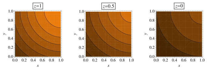
Figure 4: (Color online) Contour plot of the density distribution for a cubic pore with $L=2\sigma$. As gray becomes darker the density becomes higher.

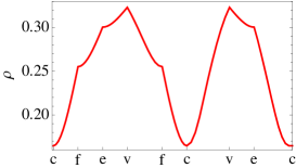
Figure 5: Density distribution for a closed path in the cubic pore with $L=2\sigma$.

III.2 Density distribution in the cylindrical cavity

For the cylindrical pore the set of relevant functions are

$$\{\mathcal{J}_{2z}(\mathbf{r}.\hat{\mathbf{z}}),\,\mathcal{J}_{2\bar{r}}(\mathbf{r}.\hat{\bar{\mathbf{r}}}),\,\mathcal{J}_{2z\bar{r}}(\mathbf{r}.\hat{\mathbf{z}},\mathbf{r}.\hat{\bar{\mathbf{r}}})\}=\sigma^{3}\{\mathcal{K}_{z}(\tilde{\mathbf{r}}.\hat{\mathbf{z}}),\,\mathcal{K}_{\bar{r}}(\tilde{\mathbf{r}}.\hat{\bar{\mathbf{r}}}),\,\mathcal{K}_{z\bar{r}}(\tilde{\mathbf{r}}.\hat{\mathbf{z}},\tilde{\mathbf{r}}.\hat{\bar{\mathbf{r}}})\}\;,$$ (60)

where the cylinder axis is in $\hat{\mathbf{z}}$ direction and $\hat{\mathbf{r}}$ is the radial polar versor. The inward normal to the lateral face is $\hat{\bar{\mathbf{r}}}=-\hat{\mathbf{r}}$ and $\mathbf{r}.\hat{\bar{\mathbf{r}}}$ is the shortest distance from the sphere center to the lateral surface of the cylinder with radius $R$. Here, the functions $\{\mathcal{K}_{z}(\mathbf{r}.\hat{\mathbf{z}}),\,\mathcal{K}_{\bar{r}}(\mathbf{r}.\hat{\bar{\mathbf{r}}}),\,\mathcal{K}_{z\bar{r}}(\mathbf{r}.\hat{\mathbf{z}},\mathbf{r}.\hat{\bar{\mathbf{r}}})\}$ are defined by translating to a cylindrical cavity the description made for the cuboidal cavity. The function $\mathcal{K}_{z}(\mathbf{r}.\hat{\mathbf{z}})$ was already analyzed in Eqs. (44-47). On the basis of the analytical expression for the overlap volume between a sphere and an infinite cylinder obtained in Ref. Lamarche_1990 (see Eq. (3) therein) we may obtain $\mathcal{K}_{\bar{r}}(\mathbf{r}.\hat{\bar{\mathbf{r}}})$ in terms of elliptic integrals. Some properties of these functions are

$$4\pi/3=\mathcal{K}_{\bar{r}}(\mathbf{r}\cdot\hat{\bar{\mathbf{r}}})+\mathcal{K}_{r}(\mathbf{r}\cdot\hat{\mathbf{r}})\>,$$ (61)

$$\mathcal{K}_{z}(\mathbf{r}\cdot\hat{\mathbf{z}}) = \mathcal{K}_{z\bar{r}}(\mathbf{r}\cdot\hat{\mathbf{z}},\mathbf{r}\cdot\hat{\bar{\mathbf{r}}})+\mathcal{K}_{zr}(\mathbf{r}\cdot\hat{\mathbf{z}},\mathbf{r}\cdot\hat{\mathbf{r}})\>,$$

$$\mathcal{K}_{\bar{r}}(\mathbf{r}\cdot\hat{\bar{\mathbf{r}}}) = \mathcal{K}_{z\bar{r}}(\mathbf{r}\cdot\hat{\mathbf{z}},\mathbf{r}\cdot\hat{\bar{\mathbf{r}}})+\mathcal{K}_{z\bar{r}}(-\mathbf{r}\cdot\hat{\mathbf{z}},\mathbf{r}\cdot\hat{\bar{\mathbf{r}}})\>,$$ (62)

$$4\pi/3=\mathcal{K}_{z\bar{r}}(\mathbf{r}\cdot\hat{\mathbf{z}},\mathbf{r}\cdot\hat{\bar{\mathbf{r}}})+\mathcal{K}_{z\bar{r}}(-\mathbf{r}\cdot\hat{\mathbf{z}},\mathbf{r}\cdot\hat{\bar{\mathbf{r}}})+\mathcal{K}_{zr}(\mathbf{r}\cdot\hat{\mathbf{z}},\mathbf{r}\cdot\hat{\mathbf{r}})+\mathcal{K}_{zr}(-\mathbf{r}\cdot\hat{\mathbf{z}},\mathbf{r}\cdot\hat{\mathbf{r}})\>.$$ (63)

We do not find an analytical expression for $\mathcal{K}_{z\bar{r}}(\mathbf{r}.\hat{\mathbf{z}},\mathbf{r}.\hat{\bar{\mathbf{r}}})$, which implies that we are not able to describe $\rho(\mathbf{r})$ near the circular edges of the cylinder when $(\mathbf{r}\cdot\hat{\mathbf{z}})^{2}+(\mathbf{r}\cdot\hat{\bar{\mathbf{r}}})^{2}<1$. However, the exact value of $\rho(\mathbf{r})$ on the edge is

$$\mathcal{K}_{z\bar{r}}(0,0)=\frac{1}{2}\mathcal{K}_{\bar{r}}(0)\>.$$ (64)

For the spheroid cavity we only found analytic expressions of $\mathcal{J}_{2a}(\mathbf{r}.\hat{\mathbf{a}})$ for points on the polar axis and points on the equatorial plane, but they are not presented here. Functions $\mathcal{J}_{2\bar{r}}(\mathbf{r}\cdot\hat{\bar{\mathbf{r}}})$ and $\mathcal{K}_{\bar{r}}(\mathbf{r}\cdot\hat{\bar{\mathbf{r}}})$ for the spherical cavity were obtained in Urrutia_2008 , and for dimensions other than 3 in Urrutia_2008 ; Urrutia_2010 . These expressions enable to obtain $\rho(r)$ near a concave or convex spherical surface. In addition, $\rho(r)$ at the spherical pore with a hard core can also be obtained analytically using the same $\mathcal{J}_{2\bar{r}}(\mathbf{r}\cdot\hat{\bar{\mathbf{r}}})$ and $\mathcal{K}_{\bar{r}}(\mathbf{r}\cdot\hat{\bar{\mathbf{r}}})$.

III.3 Pressure

The analytic evaluation of the pressure tensor $\mathbf{P}(\mathbf{r})$, a symmetric tensor of rank two, is much more difficult than the evaluation of $\rho(\mathbf{r})$ in an inhomogeneous fluid. For that reason we will not make a systematic search for each geometry confinement as was done in Secs. III.1 and III.2. Even, we only make the complete evaluation for some simple cases. The relevant task of a detailed and systematic study of $\mathbf{P}(\mathbf{r})$ for 2-HS system near simple curved walls is planned to be presented anywhere. We focus on the evaluation of the pressure tensor $\mathbf{P}$ of Irving and Kirkwood Irving_1950 . The components of $\mathbf{P}$ for the 2-particle system are $P_{ab}\left(\mathbf{r}\right)=\beta^{-1}\delta_{ab}\rho\left(\mathbf{r}\right)+P_{ab}^{U}\left(\mathbf{r}\right)$, with

$$P_{ab}^{U}\left(\mathbf{r}\right)=\left\langle r_{12}^{a}F_{12}^{b}\,\int_{0}^{1}dt\,\delta\left(\mathbf{r}-\mathbf{r}_{1}+t\mathbf{r}_{12}\right)\right\rangle_{c}\>,$$ (65)

where $\mathbf{r}_{i}$ is the coordinate of the $i$-particle, $\mathbf{r}_{12}=\mathbf{r}_{1}-\mathbf{r}_{2}$, $r_{12}^{a}=\mathbf{r}_{12}\cdot\hat{\mathbf{a}}$, and $F_{12}^{b}=\mathbf{F}_{12}\cdot\hat{\mathbf{b}}=-\dfrac{\partial\varphi}{\partial r_{12}}\,\dfrac{r_{12}^{b}}{r_{12}}$. By direct integration we obtain the identity

$$I\left(\mathbf{r},\mathbf{r}_{1},\mathbf{r}_{2}\right)=\int_{0}^{1}dt\,\delta\left(\mathbf{r}-\mathbf{r}_{1}+t\mathbf{r}_{12}\right)=r_{12}^{-1}u^{-2}\delta\left(\hat{\mathbf{r}}_{12}-\hat{\mathbf{u}}\right)\Theta\left(r_{12}-u\right)\>,$$ (66)

with $\mathbf{u}=\mathbf{r}_{1}-\mathbf{r}=u\hat{\mathbf{u}}$. For a fixed $\mathbf{r}$ we introduce a set of cartesian and spherical coordinates with the usual convention for the polar angles i.e. $r_{12}^{x}=\cos\left(\theta_{12}\right)\sin\left(\phi_{12}\right)r_{12}$, $r_{12}^{y}=\sin\left(\theta_{12}\right)\sin\left(\phi_{12}\right)r_{12}$, and $r_{12}^{z}=\cos\left(\phi_{12}\right)r_{12}$. We can re-write Eq. (65), and for example, the $P_{zz}^{U}$ component

$$\beta P_{zz}^{U}\left(\mathbf{r}\right)=Z_{2}^{-1}\iint e(\mathbf{r}_{1})e(\mathbf{r}_{2})\delta\left(r_{12}-\sigma\right)\,r_{12}\cos^{2}\left(\phi_{12}\right)\,I\left(\mathbf{r},\mathbf{r}_{1},\mathbf{r}_{2}\right)\,d^{3}r_{1}d^{3}r_{2}\>.$$ (67)

Using Eq. (66), changing the integration variables to $d^{3}u\,d^{3}r_{12}$, expressing all the distances in $\sigma$ units and both variables in spherical coordinates i.e. $d^{3}r_{12}=r_{12}^{2}\sin\left(\phi_{12}\right)dr_{12}\,d\phi_{12}\,d\theta_{12}$ and $d^{3}u=u^{2}\sin\left(\phi\right)du\,d\phi\,d\theta$, and finally integrating on $d^{3}r_{12}$, we obtain

$$\beta P_{zz}^{U}\left(\mathbf{r}\right) = Z_{2}^{-1}\sigma^{3}\int e(\mathbf{r}-\mathbf{u})e\left[\mathbf{r}-\left(1-u\right)\cdot\hat{\mathbf{u}}\right]\cos^{2}\left(\phi\right)\sin\left(\phi\right)\Theta\left(1-u\right)\,du\,d\phi\,d\theta\>.$$ (68)

Note that the range of $u$ is $1$. For $\mathbf{r}$ at a distance from the wall greater than 1 the integral $\beta P_{zz}^{U}\left(\mathbf{r}\right)$ becomes independent of $\mathbf{r}$, because for all the available values of $\mathbf{u}$ in the integration domain we have $e(\mathbf{r}-\mathbf{u})=1$ and $e[\mathbf{r}-(\sigma-u)\cdot\hat{\mathbf{u}}]=1$. Therefore, for such $\mathbf{r}$ in the region of constant density (see Eq. (43) and comments therein) we find

$$\beta P_{zz}^{U}\left(\mathbf{r}\right) = Z_{2}^{-1}\sigma^{3}\int\cos^{2}\left(\phi\right)\sin\left(\phi\right)\Theta\left(1-u\right)\,du\,d\phi\,d\theta\>,$$ (69)

$$= Z_{2}^{-1}2b_{2}\>.$$

The other components of the tensor are $P_{xx}^{U}=P_{yy}^{U}=P_{zz}^{U}$ and $P_{xy}^{U}=P_{yz}^{U}=P_{xz}^{U}=0$. This is expected because the pressure tensor in a region of constant density must be isotropic. The scalar pressure and the tensor relates by $\beta P=\beta\,tr\left(\mathbf{P}\right)/3$, where $tr$ is the trace. Therefore, the scalar pressure in the region of constant density is

$$\beta P_{0}=\rho_{0}+Z_{2}^{-1}2b_{2}=Z_{2}^{-1}2\left(Z_{1}-b_{2}\right).$$ (70)

A similar procedure was applied in Urrutia_2010 to the study of the 2-HS system in D dimensions. There, using a different definition of $P_{ab}^{U}$, the authors obtained the same result for $P_{0}$. Pressure tensor near a planar wall can also be evaluated starting from Eq. (68). We consider a wall with inward normal $\hat{\mathbf{z}}$ and an inner particle at a distance $\mathbf{r}.\hat{\mathbf{z}}=z$ with $0\leq z\leq 1$. Integrating on a domain defined by $\left|\mathbf{r}-\mathbf{u}\right|\leq 1$, $\left|\mathbf{r}-(1-u)\cdot\hat{\mathbf{u}}\right|\leq 1$, and $0<u\leq 1$ we find the normal component

$$\beta P_{N}^{U}\left(\mathbf{r}\right) = Z_{2}^{-1}2\pi\sigma^{3}\int\cos^{2}\left(\phi\right)\sin\left(\phi\right)du\,d\phi\>,$$ (71)

$$= Z_{2}^{-1}b_{2}z\,\left(3-z^{2}\right)\>.$$

Such result can be easily checked. On one side, for an inhomogeneous fluid with planar symmetry we obtain $\beta P_{N}\left(\mathbf{r}\right)=Z_{2}^{-1}2\left(Z_{1}-3b_{2}\right)$ which is independent of the position as it would be expected. On the other side, the fact that the contact value at the wall surface must be $\beta P_{N}^{U}\left(z=0\right)=\rho(0)$ which implies $P_{N}^{U}\left(z=0\right)=0$. By following an identical procedure we find for both equal tangential components that

$$\beta P_{T}^{U}\left(\mathbf{r}\right) = Z_{2}^{-1}\pi\sigma^{3}\int\sin^{3}\left(\phi\right)du\,d\phi\>,$$ (72)

$$= Z_{2}^{-1}\frac{1}{2}b_{2}z\,\left[3+z^{2}-6\,\ln\left(z\right)\right]\>.$$

For symmetry reasons the non-diagonal components are null. The scalar pressure near a planar wall is

$$\beta P(\mathbf{r})=\rho(z)+Z_{2}^{-1}2b_{2}z\,\left[1-\ln\left(z\right)\right]=Z_{2}^{-1}2\left[Z_{1}-b_{2}\left(1+z(1-z^{2})/2+z\,\ln\left(z\right)\right)\right]\>.$$ (73)

Finally, the wall-fluid surface tension of the 2-HS fluid in contact with a hard planar wall and the position of the surface of tension are

$$\beta\gamma=\beta\sigma\int\left[P_{N}\left(z\right)-P_{T}\left(z\right)\right]dz=-Z_{2}^{-1}2a_{2}\>,$$ (74)

$$z_{s}=-\gamma^{-1}\sigma\int\left[P_{N}\left(z\right)-P_{T}\left(z\right)\right]z\,dz=-0.3\!\overset{\frown}{5}\>.$$ (75)

In Fig. 6 we plot together the position dependence for the pressure tensor components and other related magnitudes near a planar wall. The dependence with position is highlighted by plotting dimensionless magnitudes independent of $Z_{2}$. We plot $\left(\beta P_{k}(z)-\rho(z=0)\right)Z_{2}/2b$ with $P_{k}=P,\,P_{N},\,P_{T}$ and $\left(\beta P_{N}(z)-\beta P_{T}(z)\right)Z_{2}/2b$ with continuous, dashed, dot-dashed and dot-dot-dashed lines, respectively. We see that at contact with the wall all functions go to zero with finite slope. For $P,\,P_{N}$ and $P_{T}$ the null value at $z=0$ is a consequence of the contact theorem. On the opposite, functions attain their definitive homogeneous value at distance $\sigma$ from the wall.

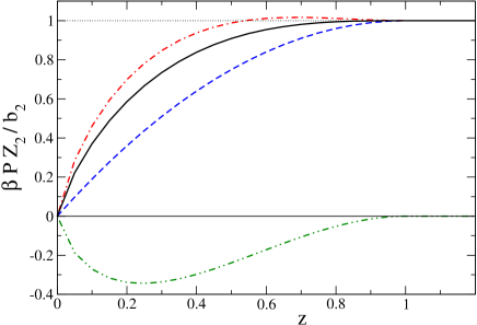
Figure 6: (color online) Position dependence of pressure tensor near a planar wall. We have drawn magnitudes related with scalar pressure $P$ in continuous line, $P_{N}$ in dashed line and $P_{T}$ in dot-dashed line. The behavior of $P_{N}\left(z\right)-P_{T}\left(z\right)$ (the integrand of Eq. (75)) is shown in dot-dot-dashed line. More details about the plotted functions in the text.

Similar to the planar case, the spherical symmetry produce only two independent components $P_{N}^{U}$ and $P_{T}^{U}$. We have obtained analytical expressions for the Irving-Kirkwood pressure tensor $\mathbf{P}$ near a spherical surface. This was done for convex and concave, surfaces. Even, the evaluation is not straightforward and therefore the study of the pressure tensor for the 2-HS system near a spherical wall will be presented in a future work. Near a cylindrical wall the components of $\mathbf{P}$ involve more complex integrals that we do not attempt to solve.

Additionally, it is interesting to note a simple relation between pressure and density in the region of constant density. Recognizing that $Z_{1}$ plays the role of the system volume we can define the mean density $\bar{\rho}=2/Z_{1}$. Therefore, from Eqs. (43, 73) we obtain the local compressibility factor in the region of constant density

$$\frac{\beta P_{0}}{\rho_{0}}=1+\frac{1}{2}\,\frac{b}{\bar{\rho}^{-1}-b}\>.$$ (76)

This is a local EOS because describes the properties in certain location of the entire 2-HS system. In Sec. V we will study thermodynamic or global EOS. Expression (76) is very similar to the EOS of a (bulk) van der Waals system without the term of attractive force between particles. They differ in the $1/2$ factor present on Eq. (76), which is related to the small number of particles of the 2-HS system. The Eq. (76) is valid for all the studied cavities, and it was also obtained for the equivalent system of confined 2-HS in dimensions $D\neq 3$. As it was suggested in Ref. Urrutia_2010 , it seems that Eq. (76) is a universal feature of a 2-HS system confined in a cavity with Hard Walls of any shape and for all dimensions $D\geq 1$. We note that for a small enough cavity that produce a vanishing size density plateau the value of $\rho_{0}$ depends on the geometry of the cavity. For a spherical cavity we have $\rho_{0}=0$ while in other cavities $\rho_{0}$ assumes positive values.

IV Analytic structure of CI

The usual classical statistical mechanics links some global thermodynamic properties of any system of particles with some derivatives of $\ln(Z_{2})$, this idea will be discussed in detail in Sec. V. Now, we simple recognize that the analytical behavior of $Z_{2}$ is related to the physical properties of the 2-HS. Therefore, the goal of this section is the study of the analytic structure of $Z_{2}$ as a function of pore size parameters $\mathbf{X}$, with the emphasis in the non-analytic domain. We are interested in investigate common features between cavities with different geometries. By including results from Urrutia_2008 ; Urrutia_2010 we compare the CI for two hard spheres constrained by five different simple geometries: cuboid, sphere, sphere with a hard core, cylinder and spheroid shaped pores. A picture representing the structure of the domains for those $Z_{2}$ is shown in Fig. 7. There, each box labeled with R (R-boxes) represents a region of parameter $\mathbf{X}$ domain studied in Sec. II as a separate case. The analytic domain of $Z_{2}$ is the union of the (open) domains represented by the R-boxes. Straight line paths show the boundaries between adjacent zones, i.e. the non analytic domain of CI, while the broaden lines highlight paths of maximum symmetry ($L_{x}=L_{y}=L_{z}$ for cuboid and $L_{h}=2R$ for cylinder). The stars distinguish the non-analytic domains involving the ergodic-non-ergodic transition. Dashed lines plot the crossover to systems with reduced dimension 0D, 1D or 2D, the 2D effective systems are represented with dark rounded-corner-boxes. The 2D limit for the spheroidal cavity has a different nature and we do not draw the box for this 2D limit.

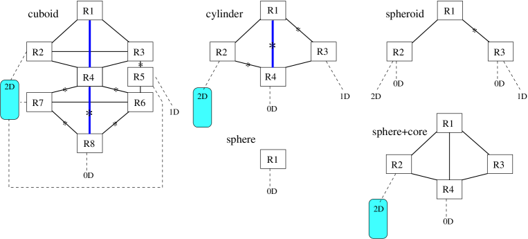
Figure 7: A simple picture representation of the $Z_{2}$ $\mathbf{X}$-space domain for all the studied pores. From top to bottom of each graph the volume decrease.

From Fig. 7 we can sort the structure of the $Z_{2}$ analytic domains for the studied cavity geometries in an increasing order of complexity: sphere, spheroid, sphere+core, cylinder, and cuboid. The sphere is the simplest geometry, the cuboid results the most complex while the spheroid, sphere+core and cylinder have a similar degree of complexity. Moreover, if we restrict from the cuboid cavity to a cube, or from the cylinder to the symmetric cylinder, its structure becomes much more simpler. This shows that the increment of the symmetry result in a decrement on the number of parameters in $\mathbf{X}$. In summary, cavities with high (poor) symmetry and few (many) number of parameters $\mathbf{X}$ produce a simple (complex) structure. In Fig. 7 we identify several interesting common features concerning different shaped pores: (a) the large pore domain R1, (b) its boundaries, (c) the $\textrm{Ri}\overset{*}{\rightarrow}\textrm{Rj}$, the signature of the ergodicity breaking, (d) the $\textrm{Rj}\rightarrow\textrm{2D}$ limit that exist in cuboid, cylinder and sphere+core pores, (e) the structure $\textrm{Ri}\overset{*}{\rightarrow}\textrm{Rj}\rightarrow\textrm{1D}$ limit, and (f) the structures $\textrm{Ri}\overset{*}{\rightarrow}\textrm{Rj}\rightarrow\textrm{0D}$ limit, $\textrm{Ri}\rightarrow\textrm{Rj}\rightarrow\textrm{0D}$ limit and particularly the last sequence $\textrm{Rj}\rightarrow\textrm{0D}$ limit. We now analyze the relevant properties for each case.

(a)

The large pore domain R1

Firstly, we concentrate in large cavities. The different analyzed geometries show that the large pore domain is the easiest to integrate and frequently the CI has a simple functional dependence. From direct inspection (see Eqs. (8-11) and also, Refs. Urrutia_2008 ; Urrutia_2010 ) we note that for cuboid, spherical and sphere+core cavities the CI is a polinomy, but a more complex analytic dependence appears for the cylindrical and spheroidal pores. A comparison with two dimensions shows that the CI of the system of two hard disks into a rectangular cavity is also a polinomy, although for a circular cavity it is not true. From all the available CI we observe that $Z_{1}b_{2}(pore)$ of Eq. (5) naturally decompose in a universal way showing a simple dependence on basic geometrical measures of the effective pore. In terms of the volume notion $V=Z_{1}$ we obtain,

$$Vb_{2}(pore) = Vb_{2}-a_{2}A+\ell_{2}Le+c_{2,1}+c_{2,2}\frac{Le}{R^{2}}\;.$$ (77)

The constant coefficients $b_{2}$ (see Eq. (4)) and $a_{2}=\sigma^{4}\pi/8$ are independent of the pore shape. $a_{2}$ appears in the virial expansion of the fluid-substrate surface tension and adsorption (referred as $w_{2}$ Bellemans_1962 ; Bellemans_1962_b ; Bellemans_1963 ; Sokolowski_1977 ) and particularly, for a HS fluid in contact with planar and spherical walls Bellemans_1963 ; Stecki_1978 ; Urrutia_2010 . Besides the volume, in Eq. (77) we introduce other geometrical characters of the effective cavity, the area of the boundary $A$ and the total edges length $Le$. In table 1 we present a comparison of the set $\{\ell_{2};\,c_{2,1};\,c_{2,2}\}$ for all the studied pore shapes, where the dependence on edges length, surface curvature and edge curvature is traced.

	cuboid	cylinder	spheroid	sphere	sph+core
$\ell_{2}/\sigma^{5}$	$1/15$	$1/15$	$-$	$-$	$-$
$c_{2,1}/\sigma^{6}$	$-1/12$	$(L_{h}/2R)\,F(\mathsf{s})\,\pi^{2}/96$	$H(\lambda)\,\pi^{2}/36$	$\pi^{2}/36$	$2\pi^{2}/36$
$c_{2,2}/\sigma^{7}$	$-$	$-\pi/210\,G(\mathsf{s})$	$-$	$-$	$-$

Table 1: Coefficients of $Vb_{2}(pore)$, dependence on the cavity shape for the large pore region.

We note that $Vb_{2}(pore)$ in Eq. (77) for cuboid, sphere and sphere+core shaped pores involves constant coefficients $\{\ell_{2};\,c_{2,1};\,c_{2,2}\}$. The coefficient $\ell_{2}$ that multiplies $Le$ has a unique positive value having the opposite sign to the preceding area term. Naturally, the edges are the area boundaries. Then, we saw the $Le$ term in Eq. (77) as a correction to the previous one. We interpret $\ell_{2}(cub)$ and $\ell_{2}(cyl)$ coefficients as being originated in the right dihedral edge formed by the intersection of two smooth surfaces. The $c_{2,1}$ is in general a slowly varying function of adimensional parameters $\mathsf{s}=\sigma/2R$ and $\lambda=Rc/R$. It is constant for cuboid, spherical and sphere+core pores. The negative constant $c_{2,1}(cub)$ has a sign opposite to the previous edges term. From that we consider it as an end-of-edge correction which corresponds to the eight right vertex of the cuboid. Then, seeking for each vertex contribution we may write $c_{2,1}(cub)/\sigma^{6}=-8/96$ and therefore each vertex produce $-1/96$. On the other hand $c_{2,1}(sph)$ and $c_{2,1}(sph+core)$ are positive, i.e. they have the sign opposite to $c_{2,1}(cub)$, and also, they are not corrections to an absent edge term. Therefore, their nature is different to that $c_{2,1}(cub)$. Coefficients $c_{2,1}(sph)$ and $c_{2,1}(sph+core)$ are originated on the curvature of the surfaces and their sign is opposite to the previous area term which corrects. Therefore, the surface curvature should produce a negative value for $c_{2,1}$ for both, a cylindrical and spheroidal pores. We introduce now the usual surface curvature measures, normal curvature $j$ and Gaussian curvature $k$, which take the values $\{j=R^{-1},\,k=0\}$ and $\{j=2R^{-1},\,k=R^{-2}\}$ for a cylinder and a sphere, respectively. We find that $c_{2,1}(sph)/\sigma^{6}=A\,R^{-2}\,\pi/144=J\!\!J(R)\,\delta^{(1)}$ and $c_{2,1}(sph+core)/\sigma^{6}=(J\!\!J(R)+J\!\!J(R-h))\,\delta^{(1)}=2c_{2,1}(sph)/\sigma^{6}$ with the extensive quadratic curvature $J\!\!J(R)=A\,j^{2}=2^{4}\pi$ and $\delta^{(1)}=3^{-2}2^{-6}\pi$ Urrutia_2010 . For cylindrical cavities we find that $c_{2,1}(cyl)/\sigma^{6}=A_{curv}R^{-2}F(x)\,\pi/384=J\!\!J(R)\,\delta^{(1)}F(x)\,3/2$, where $A_{curv}$ is the curved lateral surface area, $J\!\!J(R)=A_{curv}j^{2}=2\pi L_{h}/R$, and for large radius $c_{2,1}(cyl)\sim A_{curv}R^{-2}$. An unified description of cyl, sph and sph+core pores at large $R$ is $c_{2,1}(cyl,sph,sph+core)\,\sigma^{-6}=A_{curv}\,(\frac{3}{4}\,j^{2}+k)\,\delta^{(1)}$, but more complex dependence exist at $c_{2,1}(sphd)$. In fact, for large curvature radius and quasi spherical ellipsoids $\lambda\sim 1$ we find $c_{2,1}(sphd)\simeq c_{2,1}(sphd)\,(1+4/5\,(1-\lambda)^{2})$. Similarly, $c_{2,2}(cyl)$ relates with the curvature of the edges. We may resume some characteristics of $\{F(\mathsf{s}),G(\mathsf{s}),H(\lambda)\}$, $F(\mathsf{s})$ and $G(\mathsf{s})$ are positive and monotonically increasing functions in the domain $\left[0,1\right]$ with asymptotic minimum $F(0)=G(0)=1$. $H(\lambda)$ is positive in its domain $\left(0,\infty\right)$ and has a minimum at $H(1)=1$. Its asymptotic behavior is $H(\lambda\rightarrow\infty)\rightarrow\lambda\,3\pi/16$ and $H(\lambda\rightarrow 0)\rightarrow\lambda^{-2}/4$. In Fig. 8 we plot $F(\mathsf{s})$ and $G(\mathsf{s})$ adimensional functions.

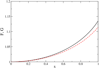
Figure 8: Shape dependent coefficients in $b_{2}(pore)$. Functions $F(\mathsf{s})$ and $G(\mathsf{s})$ of Table 1 are shown in continuous and dashed lines respectively.

We have found a general structure of $Vb_{2}(pore)$ that is explainable by a hierarchy of correction terms. Term $Vb_{2}$ is the homogeneous component, it is linear in the volume and positive. The correction to $Vb_{2}$ is the area term, the first signature of inhomogeneity. The area term is negative and then opposite in sign to the homogeneous term that corrects. Two types of essentially different corrections to the area term were found they comes from the edges and the curved area. The edge term which corrects the area term is negative and proportional to $Le$. For right dihedral edges we found the value $-1/15$ for the constant of proportionality, it appears for cuboidal and cylindrical pores. The curved area term is a correction to the area term too, and sometimes, it is independent of pore size parameters being a constant. It is negative and approximately proportional to an extensive-like quadratic curvature $A_{curv}j^{2}$. This term appears at cylindrical, spherical, spherical+core and ellipsoidal pores. Noticeably, it does not exist any extensive-like linear curvature term. Two terms which correct the edge term were also found. They concerns an edge boundary term and an edge curvature one. Both of them basically reproduce the behavior of the corrections to the area term. These conclusions make interesting the evaluation of several coefficients in other geometric confinement, which may include, $\ell_{2}$ for the edge of an arbitrary dihedral angle, $c_{2,1}$ for a general vertex produced by three non-orthogonal surfaces, for the cone vertex, and the curvature correction of the general edge.

(b)

The boundary of the large pore domain $\textrm{R1}\rightarrow\textrm{Ri}$

In the rest of Sec. IV our main purpose is to study the non-analytic behavior of CI when we go in the parameter space from an analytic domain to a contiguous one. With this in mind, we consider closed regions in the (Real) parameter space consisting in a region of the analytic domain with its boundary. We introduce the difference between the series representation of CIs, shortly $Z_{2}(\textrm{Ri})-Z_{2}(\textrm{Rj})$, corresponding to contiguous regions and evaluated in the neighboring of the common boundary. This may be not a well behaved magnitude. Even that, when at least one of the CI can be analytically extended in the contiguous region the difference $Z_{2}(\textrm{Ri})-Z_{2}(\textrm{Rj})$ is easily analyzed. More complex is the case where neither $Z_{2}(\textrm{Ri})$ nor $Z_{2}(\textrm{Rj})$ can be analytically extended in the domain of the other. In such a case we made a careful comparison between the coefficients in each series.

When we walk in the $\mathbf{X}$-space from R1 to its outside the pore becomes unable to fit both particles for some fixed direction $\hat{\mathbf{r}}_{12}$. For example, going from R1 to R3 in the cylindrical pore becomes impossible that both particles locate in a plane orthogonal to the central axis. The effect on the volume of the available position phase space is not smooth enough producing the non analytic behavior of CI. We find that the behavior of CI in several paths of the type $\textrm{R1}\rightarrow\textrm{Ri}$ are well described by

$$Z_{2}(\textrm{R1})-Z_{2}(\textrm{Ri})\equiv\boldsymbol{\Delta}Z_{2}\approx-\Delta\,\varepsilon^{3}\>,$$ (78)

that is, for many situations we verify that CI has a discontinuous third derivative when the large pore domain is crossed in the parameter space. Here $\varepsilon=1-L_{i}/\sigma$, is an adimensional vanishing parameter, $\varepsilon>0$ and $\Delta/6$ is the discontinuous step in the third derivative in the path R1$\rightarrow$Ri. When ES exceeds the planar regions of EB, i.e. R1$\rightarrow$R2, R1$\rightarrow$R3 and R1$\rightarrow$R4 for cuboidal pore; and R1$\rightarrow$R2 for cylindrical pore, we obtain

$$\Delta(cub) = (2\pi\sigma^{4}/3)L_{y}L_{z}\,,\,\textrm{for R1}\rightarrow\textrm{R2}\>,$$

$$= (2\pi\sigma^{4}/3)\left(L_{y}L_{z}+L_{x}L_{z}\right)\,,\,\textrm{for R1}\rightarrow\textrm{R3}\>,$$

$$= (2\pi\sigma^{4}/3)\left(L_{y}L_{z}+L_{x}L_{z}+L_{x}L_{y}\right)\,,\,\textrm{for R1}\rightarrow\textrm{R4}\>,$$

$$\Delta(cyl) = (2\pi^{2}\sigma^{4}R^{2}/3)\,,\,\textrm{for R1}\rightarrow\textrm{R2}\>,$$ (79)

where each equation should be evaluated at $L_{i}\rightarrow\sigma$ consistent with the analyzed path. Here, the non-analyticity of $Z_{2}$ is a consequence of the limiting behavior of the functions $\{\mathcal{I}_{3x}(cub),\,\mathcal{I}_{3y}(cub),\,\mathcal{I}_{3z}(cub)\}$ and $\mathcal{I}_{3z}(cyl)$. Close to the boundary they behave

$$\mathcal{I}_{3x}(cub) \approx -\frac{2}{3}\pi\sigma L_{y}L_{z}\left(\sigma-L_{x}\right)^{3}=-b_{2}V\,\left(1-L_{x}/\sigma\right)^{3}\,,\,\textrm{for R1}\rightarrow\textrm{R2}\>,$$

$$\mathcal{I}_{3z}(cyl) \approx -\frac{2}{3}\pi^{2}\sigma R^{2}\left(\sigma-L_{h}\right)^{3}=-b_{2}V\,\left(1-L_{h}/\sigma\right)^{3}\,,\,\textrm{for R1}\rightarrow\textrm{R2}\>,$$ (80)

where $L_{x}\rightarrow\sigma$ and $L_{h}\rightarrow\sigma$ for cuboidal and cylindrical pores, respectively. The Eqs. (79, 80) may be accomplished with

$$\Delta=\frac{\pi\sigma^{4}}{3}\,A_{+}\>,$$ (81)

$$\mathcal{I}_{3i}\approx-b_{2}\frac{\sigma}{2}\,A_{+}\left(1-L_{i}/\sigma\right)^{3}\>,$$ (82)

where $A_{+}$ is the total area of such cavity boundaries which can not contain a sphere with $\sigma$ diameter. The same procedure is feasible for non planar boundaries, R1$\rightarrow$0D in the spherical pore, R1$\rightarrow$R2 in the sph+core pore, R1$\rightarrow$R2 and R1$\overset{*}{\rightarrow}$R3 in the spheroidal pore, and R1$\overset{*}{\rightarrow}$R3 in cylindrical pore. Taking $\varepsilon=1-2R/\sigma$ we obtain

$$\Delta(sph)=\frac{\pi\sigma^{4}}{3}A\,,\,\textrm{for R1}\rightarrow\textrm{0D}\>,$$ (83)

which must be evaluated at $R=\sigma/2$. The sph+core involves two non planar walls with different curvatures, the external spherical wall has radius $R$ while the internal wall has radius $R_{in}$. Both spherical walls are apart $L_{h}=R-R_{in}$. The gap in the third derivative with $\varepsilon=1-L_{h}/\sigma$ is now

$$\Delta(sph+core)|_{R}=\frac{\pi\sigma^{4}}{3}\,\left(A_{+}-4\pi\sigma^{2}\right)\,,\,\textrm{for R1}\rightarrow\textrm{R2}\>,$$ (84)

where $A_{+}=4\pi(R^{2}+R_{in}^{2})$ is the total area.

We find three situations with a different behavior, they does not involve a finite discontinuity in the third derivative. The path R1$\rightarrow$R2 for the oblate-spheroidal pore has a discontinuous fourth derivative. For $\varepsilon=1-\frac{2R_{c}}{\sigma}>0$ we have

$$\boldsymbol{\Delta}Z_{2}(sphrd)\approx\frac{\pi^{2}\sigma^{6}}{12\lambda^{2}(1-\lambda^{2})}\,\varepsilon^{4}\,,\,\textrm{for R1}\rightarrow\textrm{R2}\>.$$ (85)

The path $\textrm{R1}\overset{*}{\rightarrow}\textrm{R3}$ involves an ergodicity breaking in prolate-spheroid and cylindrical, pores. Neglecting the factor $\xi$, for $\varepsilon=1-\frac{2R}{\sigma}>0$ we obtain for the prolate-spheroid pore

$$\boldsymbol{\Delta}Z_{2}(sphrd)\approx\frac{16\sqrt{2}\pi^{2}\lambda^{2}\sigma^{6}}{105\sqrt{-1+\lambda^{2}}}\,\varepsilon^{7/2}\,,\,\textrm{for R1}\overset{*}{\rightarrow}\textrm{R3}\>.$$ (86)

We recognize that $\Delta(cyl)$ is somewhat ill defined cause their third lateral derivatives respect to $2R$ diverge logarithmically to minus infinity. Even so, the difference between them becomes null. For $\varepsilon=1-\frac{2R}{\sigma}>1$ we obtain a non-analyticity expressible by the limiting behavior

$$\boldsymbol{\Delta}Z_{2}(cyl) \approx -\frac{32\,\sqrt{2}\pi\sigma^{6}}{105}\,\varepsilon^{7/2}\,,\,\textrm{for R1}\overset{*}{\rightarrow}\textrm{R3}\>.$$ (87)

Finally, the path $\textrm{R1}\overset{*}{\rightarrow}\textrm{R4}$ in the cylindrical pore is analyzed by a superposition of results from Eqs. (79, 87). Its behavior is similar to that found in path $\textrm{R1}\rightarrow\textrm{R2}$.

(c)

The path $\textrm{Ri}\overset{*}{\rightarrow}\textrm{Rj}$, a signature of the ergodicity breaking

The rational power in Eqs. (86, 87) corresponds to path with ergodicity breaking, thus, we wish to study their characteristics. A third path with this behavior is $\textrm{R2}\overset{*}{\rightarrow}\textrm{R4}$ for cylindrical pore. Again, neglecting the $\xi=1/2$ factor we obtain the result described in Eq. (87), based on the unanalicities of $\mathcal{I}_{3r}$. The cuboidal pore has also several paths of this type. They are the paths $\textrm{R3}\overset{*}{\rightarrow}\textrm{R5}$, $\textrm{R4}\overset{*}{\rightarrow}\textrm{R6}$, $\textrm{R4}\overset{*}{\rightarrow}\textrm{R7}$,$\textrm{R6}\overset{*}{\rightarrow}\textrm{R8}$, $\textrm{R4}\overset{*}{\rightarrow}\textrm{R8}$, and $\textrm{R7}\overset{*}{\rightarrow}\textrm{R8}$. All of them are characterized by the fact that a sphere with $\sigma$ radius fixed in the center of the cavity cross its edges. In fact, this condition is equivalent to that described above for such a cavity (see Sec. II.1, Region 5). Here the partition functions have an infinite discontinuous fifth derivatives as a consequence of the analytic behavior of the family of functions $\{\mathcal{I}_{3xy},\,\mathcal{I}_{3xz},\,\mathcal{I}_{3yz}\}$

$$\mathcal{I}_{3xy}(cub) \approx \frac{8}{9!!}\frac{L_{z}}{L_{x}^{2}L_{y}^{2}}\left(\sigma^{2}-L_{x}^{2}-L_{y}^{2}\right)^{9/2}\>,$$ (88)

$$\approx \frac{2^{11/2}}{9!!}\sigma^{5}(\alpha+\alpha^{-1})^{2}\,L_{+}\,\left(1-\frac{\sqrt{L_{x}^{2}+L_{y}^{2}}}{\sigma}\right)^{9/2}\,,\,\textrm{for R3}\overset{*}{\rightarrow}\textrm{R5}\>,$$

where $\alpha=L_{x}/L_{y}$ and $L_{+}$ is the total length of the crossed right edges, i.e. in Eq. (88) $L_{+}=4L_{z}$. Other paths are suitable analyzed by applying this result to the set $\{\mathcal{I}_{3xy},\,\mathcal{I}_{3xz},\,\mathcal{I}_{3yz}\}$. The path $\textrm{R4}\overset{*}{\rightarrow}\textrm{R6}$ is completely equivalent to $\textrm{R3}\overset{*}{\rightarrow}\textrm{R5}$. Somewhat different are the paths $\textrm{R4}\overset{*}{\rightarrow}\textrm{R7}$, $\textrm{R6}\overset{*}{\rightarrow}\textrm{R8}$, $\textrm{R7}\overset{*}{\rightarrow}\textrm{R8}$, and $\textrm{R4}\overset{*}{\rightarrow}\textrm{R8}$, which involves an ergodicity breaking along with a spontaneous symmetry breaking. Even, their analytic behavior is basically described by Eq. (88). The path $\textrm{R7}\overset{*}{\rightarrow}\textrm{R8}$ is similar to $\textrm{R3}\overset{*}{\rightarrow}\textrm{R5}$ with the replacement $y\leftrightarrow z$. Paths $\textrm{R4}\overset{*}{\rightarrow}\textrm{R7}$ and $\textrm{R6}\overset{*}{\rightarrow}\textrm{R8}$ have two equal terms with the same value of $\alpha$, the addition of both terms makes a unique contribution identical to Eq. (88) with $L_{+}$ the total length of the four crossed edges. Last path, $\textrm{R4}\overset{*}{\rightarrow}\textrm{R8}$ involves three terms with $\alpha=1$, which resumes on one term with total edges length $L_{+}=L=12\sigma/\sqrt{2}$. It is interesting to note that a similar situation is also possible for the cylindrical pore, where the circular edges are crossed by the sphere. It corresponds to the path $\textrm{R4}\rightarrow\textrm{0D}$ which will be studied below.

(d)

The $\textrm{Rj}\rightarrow\textrm{2D}$ limit

The equivalent of the HS system in two dimensions is the Hard Disk system (HD). In the 2D-limit we may expect that 2-HS systems collapse to a 2-HD system. Then, $Z_{2}$ should collapse to $Z_{2,\textrm{HD}}$ and then the CI of 2-HS in the cuboidal pore transforms to the CI of 2-HD in a box and so on. Expressions of $Z_{2,\textrm{HD}}$ for particles constrained in a rectangular or a circular pores, as well as, on the surface of a sphere are well known Munakata_2002 ; Urrutia_2008 ; Urrutia_2010 ; this fact allow us check several results in PW. The expected limiting behavior of $Z_{2}$ in terms of the vanishing length parameter $\varepsilon$ is

$$Z_{2}=\varepsilon^{2}\left[Z_{2,\textrm{HD}}+\varepsilon^{q}\,Z_{2,\textrm{HD}\,lim}\right]+O_{3+q}(\varepsilon)\>,$$ (89)

where $\varepsilon=L_{x}$ and $\varepsilon=L_{h}$ for cuboidal and cylindrical cavities, respectively. Hence, we may study the unknown term $\varepsilon^{q}\,Z_{2,\textrm{HD}\,lim}$. For the planar surface 2D-limit we obtain $q=2$, being for cuboidal shape

$$Z_{2,\textrm{HD}\,lim}(cub) = \frac{1}{6}\left[\pi L_{y}L_{z}-2\sigma(L_{y}+L_{z})+\sigma^{2}\right]\,,\,\textrm{for R2}\rightarrow\textrm{2D}\>,$$ (90)

$$= \frac{1}{3}\left[L_{z}\,\sqrt{\sigma^{2}-L_{y}^{2}}+L_{y}L_{z}\arcsin(L_{y}/\sigma)-\frac{1}{2}L_{y}^{2}-\sigma L_{z}\right]\,,\,\textrm{for R5}\rightarrow\textrm{2D}\>,$$

$$= \frac{1}{3}\left[L_{y}\,\sqrt{\sigma^{2}-L_{z}^{2}}+L_{z}\,\sqrt{\sigma^{2}-L_{y}^{2}}-\frac{1}{2}\left(\sigma^{2}+L_{y}^{2}+L_{z}^{2}\right)\right.$$

$$\left.+L_{y}L_{z}\left(\arcsin(L_{z}/\sigma)+\arcsin(L_{y}/\sigma)+\pi/2\right)\right]\,,\,\textrm{for R7}\rightarrow\textrm{2D}\>,$$

and for a cylindrical shape

$$Z_{2,\textrm{HD}\,lim}(cyl)=\frac{4\pi}{135}\left[\left(\mathsf{R}^{2}-1\right)^{-1/2}\left(32\mathsf{R}^{4}-157\mathsf{R}^{2}-3\right)+45\mathsf{R}^{2}\,\mathrm{arcsec}\left(\mathsf{R}\right)\right]\,,\,\textrm{for R2}\rightarrow\textrm{2D}\>.$$ (91)

In the case of a 2D-limit involving a curved surface confinement, we obtain for the spherical+core pore $q=1$ and

$$Z_{2,\textrm{HD}\,lim}(sph+core)=4\pi^{2}R\,[\sigma^{2}-8R^{2}]\,,\,\textrm{for R2}\rightarrow\textrm{2D}\>,$$ (92)

where $\varepsilon=L_{h}$. In the 2D limit of the oblate spheroidal pore $\textrm{R2}\rightarrow\textrm{2D}$ we do not find the behavior depicted by Eq. (89).

(e)

The $\textrm{Rj}\rightarrow\textrm{1D}$ limit

The path going from R1 to the 1D-limit has an ending structure $\textrm{Ri}\overset{*}{\rightarrow}\textrm{Rj}\rightarrow\textrm{1D}$. It means that, before to reach the limiting behavior a characteristic ergodic-non-ergodic transition appears. Once both particles are not able to interchange their positions the path $\textrm{Rj}\rightarrow\textrm{1D}$ can happen and the final 1D-limit may be attained. In that limit the HS behaves like Hard Rods (HR) and $Z_{2}$ collapses to $Z_{2,\textrm{HR}}$. The limiting behavior for $Z_{2}$ written in terms of the vanishing length parameter $\varepsilon$ ($\varepsilon^{2}=L_{x}L_{y}$ for a cuboid and $\varepsilon^{2}=\pi R^{2}$ for a cylinder) is

$$Z_{2}\approx\varepsilon^{4}\left[Z_{2,\textrm{HR}}+\varepsilon^{q}\,Z_{2,\textrm{HR}\,lim}\right]\>.$$ (93)

For the cuboidal pore $Z_{2,\textrm{HR}}=(L_{z}-\sigma/2)^{2}$, $q=2$, and

$$Z_{2,\textrm{HR}\,lim}(cub)=\frac{1}{6\sigma}(L_{z}-\sigma)\,(\alpha+\alpha^{-1})\,,\,\textrm{for R5}\rightarrow\textrm{1D}\>,$$ (94)

being $\alpha=L_{y}/L_{x}$. For the cylindrical cavity we obtain $Z_{2,\textrm{HR}}(cyl)=(L_{h}-\sigma/2)^{2}$, $q=2$, and

$$Z_{2,\textrm{HR}\,lim}(cyl)=\frac{1}{\pi\sigma}(L_{h}-\sigma)\,,\,\textrm{for R3}\rightarrow\textrm{1D}\>.$$ (95)

In addition, we may compare with the 1D-limit taken from the two dimensional 2-HD system confined into a rectangle, and from the 2-HD system confined between two concentric circles, from Refs. Munakata_2002 ; Urrutia_2008 . The 1D-limit for the 2D rectangular confinement produces $q=2$, while the circular pore with a hard core shows $q=1$. We conclude that the power $q=2$ is characteristic of straight line 1D-limit while $q=1$ corresponds to curved-closed-line 1D-limit. The prolate spheroidal pore does not behave in accordance with Eq. (93).

(f)

The $\textrm{Rj}\rightarrow\textrm{0D}$ limit

The final state obtained in this limit consists of particles that cages in a final solid or densest configuration. This densest state of 2-HS characterizes by the complete spatial correlation of particles. Two different paths coming from R1 and ending at the 0D-limit may be identified, they have the structures $\textrm{Ri}\overset{*}{\rightarrow}\textrm{Rj}\rightarrow\textrm{0D}$ and $\textrm{Ri}\rightarrow\textrm{Rj}\rightarrow\textrm{0D}$. The first case includes an ergodic-non-ergodic transition and sometimes also includes a symmetry breaking transition, it happens for the cuboid pore. We find that, in the 0D-limit the phase space of positions (PSP) may collapse to three topologically different manifolds. For a cuboidal cavity the 0D-limit shows a collapse of the PSP in a 0D-manifold, i.e. a single point. Thus, the most compact state is a solid-like state. For the cylindrical cavity in the 0D-limit the PSP collapse to a 1D-manifold consisting in a simple closed line also called a circle. Here the densest state is a rigid body which is able to rotate with a fixed axis. For the spherical cavity the 0D-limit shows that PSP collapse to a 2D-manifold given essentially by a spherical surface. Therefore the densest state behaves as a freely rotating rigid body. In the last two cases, even in the 0D-limit, particles can interchange their positions. In general, the limiting behavior of $Z_{2}$ in terms of some vanishing adimensional parameter $\varepsilon$ is $Z_{2}\propto\varepsilon^{q}$. For the cuboidal cavity with $L=L_{x}=L_{y}=\alpha\,L_{z}$ and $\varepsilon=\sqrt{2+\alpha^{2}}\,L/\sigma-1$ we obtain $q=6$ and

$$Z_{2}(cub)=\frac{(2+\alpha^{2})^{3}}{90\alpha^{2}}\sigma^{6}\varepsilon^{6}+\frac{(2+\alpha^{2})^{3}(1-\alpha^{-2}+\alpha^{-4})}{105}\sigma^{6}\varepsilon^{7}\,,\,\textrm{for R8}\rightarrow\textrm{0D}\>.$$ (96)

We note that $q=6$ also in the case of a general cuboid. Analyzing the cylindrical geometry we find $q=9/2$, $L=L_{h}=\alpha\,2R$, $\varepsilon=2R\sqrt{1+\alpha^{2}}/\sigma-1$, and

$$Z_{2}(cyl) = \pi\sqrt{2}\,(1+\alpha^{2})^{3/2}127575^{-1}\sigma^{6}\varepsilon^{9/2}\times\left[28350\alpha^{-6}+\right.\>,$$ (97)

$$\left.84105\alpha^{-4}+98100\alpha^{-2}+40200+6688\alpha^{2}+192\alpha^{4}\right]\,,\,\textrm{for R4}\rightarrow\textrm{0D}\>.$$

For the spheroid, we can attain the 0D limit in two different ways, by seeking the paths $\textrm{R2}\rightarrow\textrm{0D}$ and $\textrm{R3}\rightarrow\textrm{0D}$. We obtain, $q=7/2$, $\varepsilon=2R/\sigma-1>0$, and

$$Z_{2}(sphd)\approx\frac{16\sqrt{2}\pi^{2}\lambda^{2}\sigma^{6}}{105\sqrt{1-\lambda^{2}}}\,\varepsilon^{7/2}\,,\,\textrm{for R2}\rightarrow\textrm{0D}\>,$$ (98)

and also, $q=4$, $\varepsilon=2R_{c}/\sigma-1>0$, and

$$Z_{2}(sphd)\approx\frac{\pi^{2}\sigma^{6}}{12\lambda^{2}(-1+\lambda^{2})}\,\varepsilon^{4}\,,\,\textrm{for R3}\rightarrow\textrm{0D}\>.$$ (99)

The 0D-limit in the spherical pore was previously studied in Ref. Urrutia_2008 . In that work, it was found $q=3$ and $\varepsilon=(2R/\sigma-1)$. Also, the 0D-limit of a 2D system composed by 2-HD in a circular cavity has the same $\varepsilon$ but $q=5/2$.

We are now able to extract some minimal conclusions from this section. Based on the analysis made in (a) we note a very general decomposition of $Vb_{2}(pore)$ in terms of basic geometric magnitudes that characterize the effective cavity. This decomposition could be applied in other confinement geometries. From (b) we find a common non-analytic behavior of $Z_{2}$ when the ES exceeds planar regions of the EB boundary. It consists in a finite discontinuity at the third derivative with a step proportional to the surface area of the crossed planes. We also obtain a similar behavior for spherical surfaces and discontinuities at higher order derivatives in other curved surfaces. In general we observe that the paths between analytic domains involving ergodic-non-ergodic transitions $\textrm{Ri}\overset{*}{\rightarrow}\textrm{Rj}$ are consistent with a CI, which scales with fractional powers of the vanishing magnitude. It is apparent in (b) where we find that a $7/2$ power appears when ES exceeds a curved wall of the EB, and also, from (c) and (f) (see Eqs. (88, 97)) where we obtain a common non-analytic behavior of $Z_{2}$ when ES exceeds the right angle edges of the EB boundary given by a common power dependence of $9/2$ in the vanishing length.

A general picture of the dimensional crossovers agrees with the description given in Urrutia_2010 . Given a $N$-HS fluid system in a region of the $D$-dimensional space, the number of total spatial (i.e. translational) degrees of freedom is DF$=N\cdot D$. When we consider a limiting process of dimensional crossover the dimension of the available space reduce to $D\mathchoice{\hbox{{\textasciiacute}}}{\hbox{{\textasciiacute}}}{\hbox{{\textasciiacute}}}{\hbox{{\textasciiacute}}}$ with $0\leq D\mathchoice{\hbox{{\textasciiacute}}}{\hbox{{\textasciiacute}}}{\hbox{{\textasciiacute}}}{\hbox{{\textasciiacute}}}<D$. We define the number of lost degrees of freedom (LDF) as the power of the vanishing magnitude in the CI in the dimensional cross-over limit. We claim that LDF$=N\mathchoice{\hbox{{\textasciiacute}}}{\hbox{{\textasciiacute}}}{\hbox{{\textasciiacute}}}{\hbox{{\textasciiacute}}}\cdot(D-D\mathchoice{\hbox{{\textasciiacute}}}{\hbox{{\textasciiacute}}}{\hbox{{\textasciiacute}}}{\hbox{{\textasciiacute}}})$ where $N\mathchoice{\hbox{{\textasciiacute}}}{\hbox{{\textasciiacute}}}{\hbox{{\textasciiacute}}}{\hbox{{\textasciiacute}}}$ is the number of particles constrained to the $D\mathchoice{\hbox{{\textasciiacute}}}{\hbox{{\textasciiacute}}}{\hbox{{\textasciiacute}}}{\hbox{{\textasciiacute}}}$ dimensional region being usually $N\mathchoice{\hbox{{\textasciiacute}}}{\hbox{{\textasciiacute}}}{\hbox{{\textasciiacute}}}{\hbox{{\textasciiacute}}}=N$. One exception to this rule is the 0D limit when the final densest state consists in a rotating $N\mathchoice{\hbox{{\textasciiacute}}}{\hbox{{\textasciiacute}}}{\hbox{{\textasciiacute}}}{\hbox{{\textasciiacute}}}$-particle rigid-like system. In such a case we find LDF$=N\mathchoice{\hbox{{\textasciiacute}}}{\hbox{{\textasciiacute}}}{\hbox{{\textasciiacute}}}{\hbox{{\textasciiacute}}}D-n\,3/2$, with $n$ indicating the number of independent degrees of rotational freedom for the caged $N\mathchoice{\hbox{{\textasciiacute}}}{\hbox{{\textasciiacute}}}{\hbox{{\textasciiacute}}}{\hbox{{\textasciiacute}}}$ particles, being $0\leq n\leq D$ Urrutia_2010 . In a unified description, for any dimensional cross-over we obtain

$$\textrm{LDF}=N\mathchoice{\hbox{{\textasciiacute}}}{\hbox{{\textasciiacute}}}{\hbox{{\textasciiacute}}}{\hbox{{\textasciiacute}}}\cdot(D-D\mathchoice{\hbox{{\textasciiacute}}}{\hbox{{\textasciiacute}}}{\hbox{{\textasciiacute}}}{\hbox{{\textasciiacute}}})-n\,3/2\>,$$ (100)

where $n=0$ if $D\mathchoice{\hbox{{\textasciiacute}}}{\hbox{{\textasciiacute}}}{\hbox{{\textasciiacute}}}{\hbox{{\textasciiacute}}}\neq 0$. Here, first term counts the lost of translational degrees of freedom while the second one compensates for the non-vanishing pure rotational degrees of freedom. For PW we must fix $N=N\mathchoice{\hbox{{\textasciiacute}}}{\hbox{{\textasciiacute}}}{\hbox{{\textasciiacute}}}{\hbox{{\textasciiacute}}}=2$ with a starting value of $D=3$, and analize possible values $D\mathchoice{\hbox{{\textasciiacute}}}{\hbox{{\textasciiacute}}}{\hbox{{\textasciiacute}}}{\hbox{{\textasciiacute}}}=0,1,2$. In the zero dimensional limit the 2-HS collapses to a dumbbell or stick. Thus, $n=0$ is a non-rotating stick, $n=1$ corresponds to a rotating stick with fixed rotation axis, and $n=2$ is a freely rotating stick. Systems of two particles have a maximum value $n=D-1$. Several sequences of dimensional crossovers described by Eq. (100) are accessible from the results exposed in PW. For example, in the cylindrical cavity the path $\textrm{R2}\rightarrow\textrm{2D}$ involving LDF$=2$ can be followed by a 0D-limit with LDF$=5/2$, obtained with $D=2$, $D\mathchoice{\hbox{{\textasciiacute}}}{\hbox{{\textasciiacute}}}{\hbox{{\textasciiacute}}}{\hbox{{\textasciiacute}}}=0$ and $n=1$.

V Thermodynamic Properties

The aim of this section is to achieve the thermodynamic behavior of few bodies confined systems. Along this section we use the word thermodynamic in the sense of thermodynamic of fluids, where a fluid is a system of particles allowed to move in a given region of the continuous space. Our objective is to find the EOS that describe the global properties of a few body fluid system. In order to accomplish such a goal the discussion will be oriented towards the few and many HS system confined in a hard wall cavity with no restriction in the number of particles. In addition, we will keep in mind a system in a fluid-like state. Besides these statements other systems could be included in the discussion without much effort, such as open systems and soft interactions. Again, we must emphasize that a few body system is far away from the thermodynamic limit $N\rightarrow\infty$. Therefore, the thermodynamic description developed below does not concerns to such limit. In a few body system its different ensemble representations are not equivalent each other. Thus, we assume that the system under interest is well described by a certain Gibbsian ensemble and analyze the properties of this ensemble representation. From our point of view, we obtain the EOS of the system if we know the basic relations between the mean-ensemble values of the thermodynamic relevant magnitudes. A rigorous discussion about the equivalence between some mean-ensemble thermodynamic property e.g. $U$ and the time average value $U_{\tau}$ is out of the scope of PW. Even that, we can draw a general picture. We expect that for cavity’s size in the ergodic regime and far from an ergodic-non-ergodic transition $U=U_{\tau}$ for times $\tau$ moderately short. For example, in a cylindrical pore it should apply in R1 and R2, but far enough from R3 and R4 (see Fig. 8). In case that the size of the cavity approaches an ergodic-non-ergodic transition the identity $U=U_{\tau}$ only applies for increasing values of $\tau$. For cavities with sizes in the ergodicity breaking regime $U$ and $U_{\tau}$ may be different (e.g. R3 and R4 in the cylindrical cavity). Next paragraphs are devoted to a general discussion about the thermodynamic description of few body systems, while at the end of this section we analyze the thermodynamic behavior of confined 2-HS systems in the canonical ensemble representation making a comparison between different shaped cavities.

The pertinence of the thermodynamic theories to small systems was recognized by several authors, see e.g. the book of Hill Hill94 . From this book we can extract several arguments about the relevance of small systems to statistical mechanics and thermodynamics, and also, we find an interesting discussion about the particularities of the thermodynamics of small systems. Although, the central thesis of Hill is that the macroscopic thermodynamics must be adapted to extend its range of validity to include small systems. His thermodynamic approach begins with large (infinitely extended) systems and drops to the small ones. Certainly, we adopt an opposite point of view. We state that the first law of thermodynamics concerns to few body systems, provided that, any assumption about the extensivity of the energy and entropy must be avoided.

An implicit hypothesis of thermodynamics is that the equilibrium states of a large class of fluid systems may be specified with a unique small set of independent macroscopic quantities. A trivial example is the class of simple homogeneous fluids usually studied by taking three independent macroscopic magnitudes (see e.g. Callen’s thermodynamics book Callen85 pp. 13 and 283). Therefore, we say that thermodynamics should have the Simplicity and Universality (SU) attributes. Usually, the studied systems involve a large number of particles, but does not exist a minimum cutoff in this quantity. To highlight this point, we note that in the statistical mechanics literature the grand canonical partition function is defined by a weighted sum of canonical partition functions over the available number of particles in the system (see e.g. Hill56 ). This sum starts from zero, following by one, two particles, and goes usually up to infinity. Therefore, systems with few bodies are included in the usual formulation of the statistical mechanics. We also note that usual relations that link statistical mechanics of partition functions and thermodynamic magnitudes do not make any assumption about the number of particles. This fact supports the idea that the same relations apply to systems with few bodies. Still, any assumption of extensivity in magnitudes like the energy, entropy, and free energies must be rejected in a few bodies system (see e.g. Callen85 pp. 360). We understand the thermodynamic pertinence of systems with many and few bodies as the Size Invariance (SI) of thermodynamics. Based on SU and SI, we argue that a consistent thermodynamic treatment of systems with large, many, and few number of particles should be possible using a basic small set of independent macroscopic quantities. Naturally, we will call to this the SUSI hypothesis.

We want to bring attention to an unsolved problem in equilibrium Statistical Mechanics. At first sight it might be surprising that even when we may know the exact partition function of an inhomogeneous fluid system, their thermodynamic properties appear unrevealed. Our knowledge about the partition function comes from the exact evaluation of an integral (see paragraph above Eq. (1)). As far as, the integrand and the limits of evaluation are functions of some set of independent parameters $\mathbf{X}$, therefore by solving the integral we merely obtain $Q(\mathbf{X})$. For a HS system in a hard wall cavity at constant temperature, the discussion is mainly focused on $Z(\mathbf{X})$, where $\mathbf{X}$ can be of geometrical nature and usually involves proper lengths of the cavity, e.g. in a cuboidal pore $\mathbf{X}=\left\{L_{x},\,L_{y},\,L_{z}\right\}$. Let us suppose that, for a given $\mathbf{X}$ space with dimension $dim(\mathbf{X})$ the canonical partition function $Q(\mathbf{X})$ for the N particles system is known within a reduced domain $\mathbb{H}$. In such a domain we may obtain the Helmholtz free energy

$$\beta F(\mathbf{X})=-\ln[Q(\mathbf{X})]\>,$$ (101)

which is related to other thermodynamic quantities by

$$\mu=F(\mathbf{X})-F_{-}(\mathbf{X})\>,$$ (102)

$$F=U-TS\>,$$ (103)

$$dF=-S\,dT-dw\>.$$ (104)

In Eq. (102) the evaluation of the chemical potential $\mu$ assumes that the partition function for the system with N-1 particles, $Q_{-}(\mathbf{X})$ (with Helmholtz free energy $F_{-}$) is also known in $\mathbb{H}$. $U$, $S$, and $T$ are the energy, entropy, and absolute temperature of the system, respectively. Lastly, $dw$ is the differential of reversible work done by the system. Eq. (104) shows how $F$ depends on both, $T$ and $\mathbf{X}$. The temperature dependence gives the entropy $S$

$$S=-\left.\frac{\partial F}{\partial T}\right|_{\mathbf{X}}\>,$$ (105)

while the $\mathbf{X}$ derivative at constant $T$ is related to the work. Let us consider two different equilibrium states $a$ and $b$, characterized by parameters $\mathbf{X}_{a}$ and $\mathbf{X}_{b}$, respectively. The variations $\Delta F$, $\Delta S$, $\Delta U$ in going from state $a$ to state $b$ at fixed temperature are easily evaluated with the help of Eqs. (102, 103, 105). We may also evaluate the reversible work $w_{ab}$ in going from $a$ to $b$

$$w_{ab}=-\intop_{a}^{b}\nabla_{\mathbf{X}}F\cdot d\mathbf{X}=F(\mathbf{X}_{a})-F(\mathbf{X}_{b})\>,$$ (106)

where $\nabla_{\mathbf{X}}$ is the gradient operator with respect to $\mathbf{X}$ parameters taken at constant $T$, and the line integral in Eq. (106) does not depend on the path adopted between $a$ and $b$. From here on, we implicitly make the same assumption for any derivative with respect to $\mathbf{X}$. The Eq. (106) enable us to define the differential of reversible work

$$dw=dw_{a\hat{\mathbf{X}}}=-\partial_{\hat{\mathbf{X}}}F\cdot dl=-\nabla_{\mathbf{X}}F\cdot\hat{\mathbf{X}}\,dl\>,$$ (107)

being $\hat{\mathbf{X}}$ some unit vector in the parameter space, $dw_{a\hat{\mathbf{X}}}$ the work to make a differential reversible change from $\mathbf{X}_{a}$ to $\mathbf{X}_{b}=\mathbf{X}_{a}+\hat{\mathbf{X}}\,dl$, and $\partial_{\hat{\mathbf{X}}}$ the directional derivative. Given any volume notion $\mathcal{V}$, which may or may not be defined in the spirit of SUSI, we can define the overall pressure or pressure-for-work $\bar{P}_{w,\,\hat{\mathbf{X}}}$ for an infinitesimal transformation of the cavity

$$\bar{P}_{w,\,\hat{\mathbf{X}}}\equiv-\frac{\nabla_{\mathbf{X}}F\cdot\hat{\mathbf{X}}}{\nabla_{\mathbf{X}}\mathcal{V}\cdot\hat{\mathbf{X}}}\>,$$ (108)

which makes sense only if $\nabla_{\mathbf{X}}\mathcal{V}\cdot\hat{\mathbf{X}}\neq 0$. For an infinitesimal transformation at constant volume we should ignore Eq. (108). Even, we may prefer to introduce some surface area notion $\mathcal{A}$ and therefore we can define an external surface tension or surface-tension-for-work by

$$\bar{\gamma}_{w,\,\hat{\mathbf{X}}}\equiv\frac{\nabla_{\mathbf{X}}F\cdot\hat{\mathbf{X}}}{\nabla_{\mathbf{X}}\mathcal{A}\cdot\hat{\mathbf{X}}}\>.$$ (109)

Eqs. (108) or (109) are indeed physical conventions, and therefore, we could describe the total work as it would be produced by either an effective pressure or a surface tension. From now on we assume that $\nabla_{\mathbf{X}}\mathcal{V}\cdot\hat{\mathbf{X}}\neq 0$. Then, the definition (108) is consistent with Eq. (107), which now reads

$$dw_{\hat{\mathbf{X}}}=\bar{P}_{w,\,\hat{\mathbf{X}}}d\mathcal{V}_{\hat{\mathbf{X}}}\>,$$ (110)

where $d\mathcal{V}_{\hat{\mathbf{X}}}=\nabla_{\mathbf{X}}\mathcal{V}\cdot\hat{\mathbf{X}}\,dl$. The definition of $\bar{P}_{w,\,\hat{\mathbf{X}}}$ requires the introduction of a volume notion $\mathcal{V}(\mathbf{X})$. Hence, pressure depends on both the adopted $\mathcal{V}$ and $\hat{\mathbf{X}}$. On the opposite, even when the choice of a different $\mathcal{V}$ modifies $\bar{P}_{w,\,\hat{\mathbf{X}}}$ it does not influence $dw_{a\hat{\mathbf{X}}}$.

At this point we emphasize that, even when the above description is exact it is not completely satisfactory. It says little about the thermodynamic properties of the fluid inside the cavity. It depends on $\mathbf{X}$ parameters, which do not have a universal thermodynamic meaning. The parameters needed to describe the shape of certain cavity are of different kind and quantity that those needed to describe other shapes. Even worst, for a given geometry they are non unique. We may extract some examples from the studied two particle systems. For a cavity with spherical symmetry we may utilize $\mathbf{X}=\left\{R+\sigma/2\right\}$ or $\mathbf{X}=\left\{R\right\}$, but also, we may adopt $\mathbf{X}=\left\{\pi R^{2}\right\}$ all of them with $dim(\mathbf{X})=1$. In a cuboidal cavity we may adopt $\mathbf{X}=\left\{L_{x},\,L_{y},\,L_{z}\right\}$ or $\mathbf{X}=\left\{l_{x},\,l_{y},\,l_{z}\right\}$ with $dim(\mathbf{X})=3$, but also, if we are interested in $a$ and $b$ states with cubic symmetry we may choose $\mathbf{X}=\left\{L\right\}$ with $dim(\mathbf{X})=1$. However, a somewhat more realistic cavity model may be adopted in which the substrate atoms, HS at fixed positions, are the building blocks of the rough confinement walls. In this case $dim(\mathbf{X})$ could be a much larger number. In addition, the $\mathbf{X}$-representation prevents to compare results from dissimilar confinement conditions. Hence, the same fluid in a spherical or cuboidal cavity produces results which inhibit any comparison between them.

We conclude that next step forward in the thermodynamic description of the system is out of the scope of the $\mathbf{X}$-representation. Therefore, it is necessary to build the path between the $\mathbf{X}$-representation of certain thermodynamic property, e.g. $Q(\mathbf{X})$, and a universal description. Two basic questions have guided to us in the search of such a path; i) What properties of the confined systems should depend on the shape of the cavity? ii) What properties should depend on the particular choice of adopted parameters $\mathbf{X}$? The rest of this section shows some answers, which arise from our inquiries.

Being $\mathbf{X}$ an unsuitable set of parameters we must look for a better choice. At this point we wish to extract a paragraph from Callen’s Themodynamics book, ”It should perhaps be noted that the choice of the variables in terms of which a given problem is formulated, while a seemingly innocuous step, is often the most crucial step in the solution.” (Callen85 p. 465). The interesting point is that Callen focus on the relevance of an adequate choice of variables. This question guide us to the concept of thermodynamic variable of state (VOS). We are interested in such VOS that characterize the spatial extension and other spatial features of an inhomogeneous fluid. A long time ago, in the origins of thermodynamics, volume was recognized as a good VOS for diluted gases as was stated in Boile’s law in 1662. A step forward was the introduction of surface area and curvature as VOS, it is documented in the study of vapor-fluid spherical interfaces made in 1805 and 1806 by Young and Laplace Young_1805 ; Laplace . Although, in 1875 Gibbs Gibbs1906 extended the use of curvature measures as VOS when he analyzed non-spherical fluid-vapor and fluid-fluid interfaces. Gibbs, also suggested the use of the length of the three fluid interface line as VOS. This idea was further developed in 1977 by Boruvka and Newmann Boruvka_1977 , which also introduced the curvature of such line as VOS. These VOS were extensively applied to the thermodynamic analysis in a variety of macroscopic inhomogeneous fluid systems including liquid-vapor and liquid-liquid interfaces, and adsorption of fluids on solids in accordance with SU Sokolowski_1979 ; Henderson_1983 ; Henderson_2002 ; Henderson_2004 ; Blokhuis_2007 , but they were never applied to the thermodynamic analysis of few body systems, in contradiction to SI. Besides, these thermodynamic magnitudes are based in geometrical concepts, but even when the geometrical concepts have a precise definition, their counterpart thermodynamic magnitudes have usually not a precise meaning. For example, in the system of many hard spheres in contact with a (convex) spherical wall different choices for the locus of the so called Gibbs dividing surface is not innocuous. A comparison between Refs. Bryk_2003 and Blokhuis_2007 shows that the locus of this surface may modify the volume and surface area of the inhomogeneous non-planar fluid system. Both modifications influence the macroscopic description of the entire system, changing the Laplace equation, the surface tension, etc. The most dramatic change is probably in the Tolman length.

Therefore, we introduce a set $\mathbf{M}$ of thermodynamic measures, which should be suitable VOS in accordance with SUSI requirements. We seek for a set $\mathbf{M}$ with a precise definition which enables an exact description of few body exactly solved systems, and also, we expect that a good choice for $\mathbf{M}$ provides consistence with previous well stablished known results. The homogeneous fluids are typically described by taking $\mathbf{M}=\left\{V\right\}$ with $dim(\mathbf{M})=1$, while for inhomogeneous systems several authors currently add the surface area, being $\mathbf{M}=\left\{V,A\right\}$ and $dim(\mathbf{M})=2$. The classical analysis of the ideal gas produce an elementary EOS, $PV=NkT$. Accordingly, $\mathbf{M}$ must include a volume measure $V$ with a pressure provided by $P=-\partial_{V}F(\mathbf{M})$ compatible with the known system pressure, yielding the expected behavior for non interacting particles. The same thought applies for the surface area of the substrate and the wall-fluid surface tension $\gamma$. The discussion about the choice of $\mathbf{M}$ will be completed later in PW. Now, assuming that we have adopted a set $\mathbf{M}$ and also that $\mathbf{M}(\mathbf{X})$ is given, we must implement the thermodynamic description of the system using these measures. With this purpose we need to relate the $\mathbf{X}$-representation and the $\mathbf{M}$-representation. We state that $w_{ab}$ must be independent of the adopted representation $\mathbf{X}$ or $\mathbf{M}$, then we claim

$$w_{ab}(\mathbf{M})=w_{ab}(\mathbf{X})\>,$$ (111)

$$dw_{a\hat{\mathbf{M}}}=dw_{a\hat{\mathbf{X}}}\>,$$ (112)

where we assume that $\mathbf{M}_{a}$ and $\mathbf{M}_{b}$ are well defined quantities and also, that for all $\mathbf{X}\in\mathbb{H}$ must exist $\mathbf{M}(\mathbf{X})$. Hence, Eqs. (106, 107) transform to

$$w_{ab}=-\intop_{a}^{b}\nabla_{\mathbf{M}}F\cdot d\mathbf{M}=-\intop_{a}^{b}\mathbf{m}\cdot d\mathbf{M}\>,$$ (113)

$$dw_{a\hat{\mathbf{M}}}=-\partial_{\hat{\mathbf{M}}}F\cdot dl=-\mathbf{m}\cdot\hat{\mathbf{M}}\,dl\>,$$ (114)

where $\mathbf{m}\equiv\nabla_{\mathbf{M}}F$, and for a given direction $\hat{\mathbf{X}}$ in the parameters space $\hat{\mathbf{M}}=\nabla_{\mathbf{X}}\mathbf{M}\cdot\hat{\mathbf{X}}$. Comparing Eq. (107) with Eq. (114) we find

$$\nabla_{\mathbf{X}}F\cdot\hat{\mathbf{X}}=\mathbf{m}\cdot\hat{\mathbf{M}}=\sum_{j}\left.\frac{\partial F}{\partial M_{j}}\right|_{\mathbf{M}-M_{j}}\left(\sum_{i}\left.\frac{\partial M_{j}}{\partial X_{i}}\right|_{\mathbf{X}-X_{i}}\hat{X}_{i}\right)\>,$$ (115)

where $\hat{X}_{i}$ is the $i$-component of $\hat{\mathbf{X}}$, $m_{j}=\left.\frac{\partial F}{\partial M_{j}}\right|_{\mathbf{M}-M_{j}}$, and $\mathbf{M}-M_{j}$ means that all the measures but the $j$-component are kept constants in the partial derivative. The Eq. (115) is simply the chain rule for the $F$ derivatives. When we adopt the volume notion of Eq. (109) as the volume measure $M_{1}=V=\mathcal{V}$ we obtain $P=-m_{1}$, and also from Eqs. (115, 109)

$$P-\bar{P}_{w,\,\hat{\mathbf{X}}}=\Delta P_{\hat{\mathbf{X}}}=\sum_{j=2}^{dim(\mathbf{M})}m_{j}\,\frac{\nabla_{\mathbf{X}}M_{j}\cdot\hat{\mathbf{X}}}{\nabla_{\mathbf{X}}V\cdot\hat{\mathbf{X}}}\>,$$ (116)

which is a Laplace-like equation for a fluid-substrate interface Blokhuis_2007 . The Eqs. (109, 116) show that $\left|\hat{\mathbf{X}}\right|$ is irrelevant and therefore the restriction to unit modulus in Eq. (110) is superfluous. An interesting point is that $\bar{P}_{w,\,\hat{\mathbf{X}}}$ and $P$ can be measured both experimentally and with molecular dynamic simulations.

Now, to make a practical use of Eq. (116) the unknowns $m_{j}$, i.e. the EOS of the system, should be revealed. Therefore, we need $F(\mathbf{M})$ (see Eq. (113)). In general the set $\mathbf{M}$ may include dependent magnitudes and then $dim(\mathbf{M})\neq dim(\mathbf{X})$ showing that relation $\mathbf{M}\leftrightarrow\mathbf{X}$ is not a one-to-one or biyective relation. Thus, the transformation $F(\mathbf{X})\rightarrow F(\mathbf{M})$ is not a simple change of variables, which disable us to obtain $F(\mathbf{M})=F(\mathbf{X}(\mathbf{M}))$. We need a procedure to identify the hidden dependence of $F(\mathbf{X})$ in $\mathbf{M}$. Accordingly, we must overcome two difficulties, find a good set $\mathbf{M}(\mathbf{X})$ and obtain $F(\mathbf{M})$. Now, we can show that the selection of measures $\mathbf{M}$ and the identification of $F(\mathbf{M})$ are not independent questions. To proceed, we analyze some results for the 2-HS confined system.

We are mainly interested in fluid-like systems where particles can move freely and are able to interchange their positions. Then, we look for measures $\mathbf{M}$ that enable the thermodynamic description of systems in this regime. Certainly this $\mathbf{M}$ may or may not be suitable to describe other situations as solid-like or dense systems. The graph decomposition presnted in Sec. II (see also Urrutia_2008 ) and the analysis performed in Sec. IV.(a) show that some thermodynamic measures $\mathbf{M}$ appear naturally in $F$ for cavity sizes in the Region 1. For higher confinement conditions, as in Region 2 and 3, some characteristics surface areas and lengths of the cavity also emerge as thermodynamic measure candidates. We focus on the results for Region 1 where any characteristic length of the cavity is greater than $\sigma$. The list of measures candidates starts with the volume $V\equiv Z_{1}=\int e(r)\,d\mathbf{r}$, suggested by the graph decomposition in Eqs. (3, 4). This volume appears usually in the study of inhomogeneous fluids Sokolowski_1977 ; Sokolowski_1978 ; Sokolowski_1979 ; Sokolowski_1981 ; Rowlinson_1985 of different nature. Interestingly, for fluid systems in contact with hard walls, this $V(\mathbf{X})$ makes that $\bar{P}_{w,\,\hat{\mathbf{X}}}$ reduces to the contact pressure on the hard-wall. In fact, it reproduces exactly the hard-wall pressure contact theorem for planar, spherical and cylindrical hard walls, but also for much more complex geometrical shapes of the cavity Urrutia_2010c . Other magnitudes are also suggested by the Eqs. (5, 77), e.g. the surface area measure defined as $A\equiv\int\nabla e(r)\cdot\hat{n}\,d\mathbf{r}$. We also consider $Le$, the measure of total edges length with right internal angle. More measures could be added, the number of right vertex, $N_{vert}$, some measure of the surface curvature e.g. $\mathsf{M}\equiv\int(\frac{3}{4}\,j^{2}+k)\,d\mathbf{S}$, and a measure of the edge’s curvature.

Finally, even for Region 1, to ensure the exactness of Eq. (116) in principle we should include $\mathbf{X}$ in the set of measures. With all these measures we may conform a complete measure set $\mathbf{M}_{c}=\left\{V,A,L_{e},N_{vert},\mathsf{M},\mathbf{X}\right\}$, which is certainly not a small set of measures. We note that a hierarchy exist in $\mathbf{M}_{c}$, the most important therm is $V$, the second in relevance is $A$. Both of them have been defined in detail, and its definition can be applied to a large class of systems. Next terms, $Le$, $N_{vert}$ and $\mathsf{M}$ behave less important and their definition concern particular characteristics of confinement cavity. Finally, the last added terms to $\mathbf{M}_{c}$ are still less relevant. Their definition applies only to a given cavity geometry, and were included to make a complete description of $F$, so that Eqs. (111, 112) are guaranteed. The loss of relevance for incoming terms in $\mathbf{M}_{c}$ relates with the SU hypothesis.

Now, we take into account all these questions to analyze the thermodynamic behavior of 2-HS systems in Region 1. The spheroidal cavity will be excluded from the thermodynamic analysis because we do not find a small set $\mathbf{M}$ that enable the unified study of this and other geometries. We adopt the small set of measures $\mathbf{M}=\left\{V,A,L_{e},R\right\}$ where the last parameter is the radius of curvature of the (curved) surface. Measure $R$ is frequently used in the study of fluid systems in contact with simple curved surfaces as such with cylindrical or spherical symmetries Poniewierski_1997 ; Blokhuis_2007 . We also select a rule to identify the dependence of $F$ on the adopted set of measures $\mathbf{M}$. It is based on re-writing Eq. (77) in the form

$$Vb_{2}(pore)=Vb_{2}-A\,a(R)+L_{e}\,\ell(R)\;.$$ (117)

Again, the adopted $\mathbf{M}$ and the identification rule are non-unique. In the Appendix A a different $\mathbf{M}$ is analyzed. For the adopted $\mathbf{M}=\left\{V,A,L_{e},R\right\}$, we can define the $F$ derivatives related with the volumetric-work, surface-area-work, edges-length-work and radius-of-curvature-work

$$-P=\left.\frac{\partial F}{\partial V}\right|_{T,\mathbf{M}-V}\>,$$ (118)

$$\gamma=\left.\frac{\partial F}{\partial A}\right|_{T,\mathbf{M}-A}\>,$$ (119)

$$\tau=\left.\frac{\partial F}{\partial Le}\right|_{T,\mathbf{M}-Le}\>,$$ (120)

$$C_{R}=\left.\frac{\partial F}{\partial R}\right|_{T,\mathbf{M}-R}\>.$$ (121)

From Eq. (116) we relate the difference of pressures $\Delta P_{\hat{\mathbf{X}}}$ for an infinitesimal deformation in $\hat{\mathbf{X}}$ direction with $\gamma$, $\tau$, etc. by

$$\Delta P_{\hat{\mathbf{X}}}=\gamma\,\frac{\nabla_{\mathbf{X}}A\cdot\hat{\mathbf{X}}}{\nabla_{\mathbf{X}}V\cdot\hat{\mathbf{X}}}+\tau\,\frac{\nabla_{\mathbf{X}}Le\cdot\hat{\mathbf{X}}}{\nabla_{\mathbf{X}}V\cdot\hat{\mathbf{X}}}+\ldots\>,$$ (122)

Now it is apparent that Eq. (122) is a generalization of the Laplace equation obtained for a macroscopic fluid system in contact with a spherical wall Henderson_1983 ; Henderson_1986_inCroxton86 . An interesting fact is that the EOS given in Eqs. (118-121) may be strongly dependent on the details of the fluid system. On the other hand, the relation between $\Delta P_{\hat{\mathbf{X}}}$, $\gamma$, $\tau$, etc. given by the Laplace-like equation (122) only depends on the geometry of the cavity and the adopted $\mathbf{M}$. For example, given a cuboidal pore it remains unperturbed if we confine 2-HS, an N-Lennard-Jones, or any other fluid. Before analyzing each confinement geometry we wish to state that, for all the studied cavities, the thermodynamic pressure from Eq. (118) is

$$\beta P=Z_{2}^{-1}\,2\left(V-b_{2}\right)\>.$$ (123)

This is our first global or thermodynamic EOS for the 2-HS system. The same expression was obtained in Eq. (73) for the local pressure in the constant density region when we analyze cavities of any shape. We find that both pressures are equal, which shows the consistence of the present thermodynamic study. A similar result for spherical confinement was previously obtained Urrutia_2010 . Based on the universal behavior of Eqs. (77, 117) and the consistence between the local pressure in the constant density region and thermodynamic pressure in all the studied cavity geometries, we confirm that the adopted volume measure is correct in the spirit of SUSI. Therefore, taking the volume measure $V=Z_{1}$ we argue that the identity between both pressures should be true for a 2-HS system in any cavity shape. In the next paragraphs we perform the thermodynamic analysis for each pore shape. We fix $\sigma=1$ to keep notation simple.

V.1 The cuboidal pore

The cuboidal pore does not involve $R$, then $\mathbf{M}=\left\{V,\,A,\,Le\right\}$. We obtain the thermodynamic pressure of Eq. (123) and also,

$$\beta\gamma=-Z_{2}^{-1}\,2a_{2}\>,$$ (124)

$$\beta\tau=Z_{2}^{-1}\,2\ell_{2}\>.$$ (125)

The three EOS relate the pressure, surface tension, and line-tension with the measures $\left\{V,\,A,\,Le\right\}$ of the system. They apply to any cuboidal pore, in particular these equations are valid for the cubic confinement. Surface tension $\gamma$ of Eq. (124) is in coincidence with Eq. (74), it is negative for large enough cavities. A Simple inspection shows that for large cuboids the EOS scales $\beta P\simeq\rho+b_{2}\rho^{2}/2$, $\beta\gamma\simeq-a_{2}\rho^{2}/2$ and $\beta\tau\simeq\ell_{2}\rho^{2}/2$ . For $\bar{P}_{w,\,\hat{\mathbf{X}}}$ we may find in the literature two frequently used deformations. Adopting the length parameters $\mathbf{X}=\left\{L_{x},\,L_{y},\,L_{z}\right\}$, the first one is like a piston expansion transformation and reads $\hat{\mathbf{X}}=(1,0,0)$. From Eq. (109)

$$\beta\bar{P}_{w,\,\hat{\mathbf{X}}}=Z_{2}^{-1}\left[2\left(V-b_{2}\right)+\frac{2a_{2}2(L_{y}+L_{z})-2\ell_{2}4}{L_{y}L_{z}}\right]\>,$$ (126)

with this choice of $\hat{\mathbf{X}}$ magnitudes $P$, $\gamma$, $\tau$, and $\bar{P}_{w,\,\hat{\mathbf{X}}}$ are related each other by

$$\Delta P_{\hat{\mathbf{X}}}=\gamma\,\left(\frac{2}{L_{y}}+\frac{2}{L_{z}}\right)+\tau\,\frac{4}{L_{y}L_{z}}\>.$$ (127)

Equivalent results may be obtained with $\hat{\mathbf{X}}=(0,1,0)$ or $\hat{\mathbf{X}}=(0,0,1)$. The second option is an isotropic expansion with $\hat{\mathbf{X}}=(1,1,1)$, which produces

$$\beta\bar{P}_{w,\,\hat{\mathbf{X}}}=-Z_{2}^{-1}\left[2\left(V-b\right)+\frac{2a_{2}4(L_{x}+L_{y}+L_{z})-2\ell_{2}12}{L_{y}L_{z}+L_{x}L_{z}+L_{x}L_{y}}\right]\>,$$ (128)

$$\Delta P_{\hat{\mathbf{X}}}=\gamma\,\frac{2Le}{A}+\tau\,\frac{24}{A}\>.$$ (129)

We now analize $\hat{\mathbf{X}}=(1,0,0)$, $\hat{\mathbf{X}}=(1,1,1)$ starting with a cubical cavity $L=L_{x}=L_{y}=L_{z}$. In this case Eqs. (126) and (128) converge to a single expression. The same applies also to Eqs. (127, 129) which can be simplified because $(A-A_{x})/V=4L^{-1}$, $Le_{x}/V=4L^{-2}$, and $Le/A=2\,L^{-1}$. Therefore, for all the studied $\hat{\mathbf{X}}$ for a cubical cavity we obtain

$$\beta\bar{P}_{w,\,\hat{\mathbf{X}}}=-Z_{2}^{-1}\left[2\left(V-b\right)+8\frac{a_{2}L-\ell_{2}}{L^{2}}\right]\>,$$ (130)

$$\Delta P_{\hat{\mathbf{X}}}=\gamma\,\frac{4}{L}+\tau\,\frac{4}{L^{2}}\>.$$ (131)

The same expressions (123, 124, 125, 130, 131) are obtained if we start from the beginning the analysis of a cubical cavity with $\mathbf{X}=\{L\}$ and $\hat{\mathbf{X}}=(1)$, which shows the robustness of the procedure.

V.2 The cylindrical pore

From the same basic set of measures we recognize that the planar and curved surfaces, with areas $A_{p}$ and $A_{c}$, respectively, are geometrically and therefore thermodynamically different. Then we split the total area in two, adopting $\mathbf{M}=\left\{V,\,A_{p},A_{c},\,Le,\,R\right\}$. For $P$ and $\gamma_{p}$ we obtain expressions identical to Eqs. (123, 124). Other EOS are

$$\beta\gamma_{c}=-Z_{2}^{-1}2a_{2}\left(1-c_{I}R^{-2}\right)\>,$$ (132)

$$\beta\tau=Z_{2}^{-1}2\ell_{2}\left(1-c_{I\!I}R^{-2}\right)\>,$$ (133)

$$\beta C_{R}=-Z_{2}^{-1}R^{-3}\left(c_{I\!I\!I}A_{c}+c_{I\!V}Le\right)\>,$$ (134)

where $c_{I}=F(\mathsf{s})/48$, $c_{I\!I}=G(\mathsf{s})\,\pi/14$, $c_{I\!I\!I}=\pi/96\,\left(F(\mathsf{s})+\mathsf{s}F^{\prime}(\mathsf{s})/2\right)$, and $c_{I\!V}=\pi/210\,\left(G(\mathsf{s})+\mathsf{s}G^{\prime}(\mathsf{s})/2\right)$. All of these coefficients are positive smooth functions with small values, e.g. $c_{I}<0.03$, which shows that $\gamma_{p}\simeq\gamma_{c}$. We can also extract the curvature dependence of $\gamma$

$$\frac{\gamma_{c}}{\gamma_{p}}-1=-\frac{1}{48}R^{-2}+O(R^{-4})\>.$$ (135)

Taking $\mathbf{X}=\left\{L_{h}/2,\,R\right\}$ for this geometry, we see three simple choices for $\hat{\mathbf{X}}$. The piston expansion $\hat{\mathbf{X}}=(1,0)$ provides

$$\Delta P_{\hat{\mathbf{X}}}=\gamma_{p}\,\frac{2}{R}\>.$$ (136)

For the lateral $\hat{\mathbf{X}}=(0,1)$ and isotropic $\hat{\mathbf{X}}=(1,1)$ expansions we obtain

$$\Delta P_{\hat{\mathbf{X}}}=\gamma_{p}\frac{2}{L_{h}}+\gamma_{c}\frac{1}{R}+\tau\,\frac{2}{L_{h}R}+C_{R}\frac{1}{A_{c}}\>,$$ (137)

$$\Delta P_{\hat{\mathbf{X}}}=\gamma_{p}\frac{Le}{A}+\gamma_{c}\,\frac{Le+2\pi L_{h}}{A}+\tau\,\frac{4\pi}{A}+C_{R}\frac{1}{A}\>.$$ (138)

For the cylinder with maximum area at fixed volume $L_{h}/2=R$ and Eq. (138) reduces to

$$\Delta P_{\hat{\mathbf{X}}}=\left(\gamma_{p}+2\gamma_{c}\right)\,\frac{2}{3R}+\left(\tau+\frac{C_{R}}{4\pi}\right)\frac{2}{3R^{2}}\>,$$ (139)

which may be still obtained analyzing the cylindrical pore from the beginning with $L_{h}/2=R$, $\mathbf{X}=\left\{R\right\}$ and $\hat{\mathbf{X}}=(1)$.

V.3 The spherical and spherical+core pores

The spherical pore has $Le=0$, which reduces the measures to $\mathbf{M}=\left\{V,\,A,\,R\right\}$. The expression for $P$ is identical to Eq. (123) to which we add

$$\beta\gamma=-Z_{2}^{-1}2a_{2}\left(1-18^{-1}R^{-2}\right)\>,$$ (140)

$$\beta C_{R}=-Z_{2}^{-1}2a_{2}A\,9^{-1}R^{-3}\>.$$ (141)

For $\mathbf{X}=\left\{R\right\}$ and $\hat{\mathbf{X}}=(1)$ the difference of pressures is

$$\Delta P_{\hat{\mathbf{X}}}=\gamma\,\frac{2}{R}+\frac{C_{R}}{A}\>,$$ (142)

and the same result is obtained for any other choice of $\mathbf{X}$ and $\hat{\mathbf{X}}$. Note that using the Eqs. (140, 141) we may transform $\frac{C_{R}}{A}$ to obtain

$$\Delta P_{\hat{\mathbf{X}}}=\gamma\,\left(\frac{2}{R}+\beta C_{R}\right)+\frac{\partial\gamma}{\partial R}\>.$$ (143)

Eq. (143) is very similar to the Laplace equation for a macroscopic fluid in contact with a spherical wall Henderson_1983 ; Henderson_1986_inCroxton86 ; Blokhuis_2007 . Now, we will analyze the 2-HS system in a spherical pore with a hard core. The shape of this pore involves two surfaces with different curvature. Therefore, as we did for the cylindrical cavity we consider two separate surface area measures. We adopt $\mathbf{M}=\left\{V,\,A_{e},\,A_{i},\,R_{e},-R_{i}\right\}$, where $-R_{i}$ is the (negative) radius of curvature of the internal surface, and naturally, the labels $e$ and $i$ design the properties of the external and internal surfaces, respectively. The pressure $P$ is given in Eq. (123), while other EOS are

$$\beta\gamma_{e}=-Z_{2}^{-1}2a_{2}\left(1-18^{-1}R_{e}^{-2}\right)\>,$$ (144)

$$\beta\gamma_{i}=-Z_{2}^{-1}2a_{2}\left(1-18^{-1}R_{i}^{-2}\right)\>,$$ (145)

$$\beta C_{Re}=-Z_{2}^{-1}2a_{2}A_{e}9^{-1}R_{e}^{-3}\>,$$ (146)

$$\beta C_{-Ri}=Z_{2}^{-1}2a_{2}A_{i}9^{-1}R_{i}^{-3}\>.$$ (147)

In these Eqs. we recognize that the opposite sign in both radius of curvature do not affect surface tension expressions, but invert the sign in curvature term. Adopting the length parameters $\mathbf{X}=\left\{R_{e},-R_{i}\right\}$, we can analyze three simple transformations $\hat{\mathbf{X}}=(1,0)$, $\hat{\mathbf{X}}=(0,1)$, and $\hat{\mathbf{X}}=(1,1)$. For the first two cases we find

$$\Delta P_{\hat{\mathbf{X}}}=\gamma_{e}\,\frac{2}{R_{e}}+\frac{C_{Re}}{A_{e}}\>,$$ (148)

$$\Delta P_{\hat{\mathbf{X}}}=-\gamma_{i}\,\frac{2}{R_{i}}+\frac{C_{-Ri}}{A_{i}}\>.$$ (149)

Here the effect of the negative curvature radius in the Laplace-like equations is apparent. The last transformation gives

$$\Delta P_{\hat{\mathbf{X}}}=\frac{\gamma_{e}+\gamma_{i}}{R_{e}+R_{i}}+\frac{\gamma_{e}-\gamma_{i}}{L_{h}}+\frac{C_{Re}+C_{-Ri}}{A_{e}-A_{i}}\>.$$ (150)

For all the studied simple geometrical confinement we obtained several relation between intensive-like magnitudes that resemble the Laplace equation. We must stress that previous to implement the thermodynamic study of the system we has needed to choose both, a set $\mathbf{M}$ and an identification rule (see Eq. (117)). Both choices affect its thermodynamic description. In the Appendix A a different choice for $\mathbf{M}$ is taken, which produce other set of EOS.

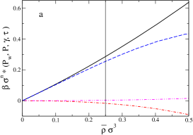
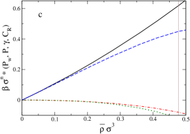
Figure 9: (color online) Magnitudes related to the thermodynamic work: pressures, wall-fluid surface tensions, line tensions and curvature-work. From top to bottom a) is for a cube cavity, b) is for a symmetric cylindrical cavity and c) is for a spherical cavity. The power $n$ is chosen in each case to give a dimensionless magnitude.

In Figure 9 we plot pressure for work, pressure, surface tension and other EOS for the cube, the $L_{h}=2R$ cylinder and spherical cavities (subfigures a, b, and c, respectively) as functions of the rough density. In continuous line we plot $\bar{P}_{w,\,\hat{\mathbf{X}}}$, in dashed line $P$, in dot-dashed line $\gamma$, dot-dot-dashed line shows $\tau$, and dotted line $C_{R}$. The vertical line shows the end of the plateau of constant density $\rho_{0}$ and constant pressure $P_{0}$. The most remarkable feature is that Figs. 9a, 9b, and 9c are very similar in the density range $(0,\,0.5)$. A very small difference in $\bar{P}_{w,\,\hat{\mathbf{X}}}$ at $\bar{\rho}\sigma^{3}=0.5$ is due to the expected geometric dependence of the ratio $V/A$. In Fig. 9b both wall-fluid surface tensions, $\gamma_{p}$ and $\gamma_{c}$, are plotted but are indistinguishable. A clear difference between the three figures appears in the curvature term, which is not present for the cube cavity at Fig. 9a. In Fig. 9b $C_{R}$ mix two curvature contributions, one due to the curved surface and other due to the curved edges. Even, in Fig. 9c $C_{R}$ is a purely surface curvature effect. A second difference is the vertical line that shows the end of the plateau, which is a purely local property of the 2-HS system. Note that $F(\mathbf{X})$ (and also $F(\mathbf{M})$) is an analytic function at this point because their analytic domain extends to the end of Region 1. The non-analytic point for Figs. 9a, 9b and 9c corresponds to maximum densities $\bar{\rho}\sigma^{3}=2,\,2.55$ and $3.82$, respectively. Beyond the vertical plateau-end-line the identification of the thermodynamic pressure $P$ with the plateau’s pressure $P_{0}$ breaks down because the central plateau of constant density disappears. If we wish to retain the identity beyond this point we can regard about the analytic continuation of Eqs. (43) and (70). This approach may conduce to a non-monotonic behavior of $P$ related in some cases (for the spherical cavity) with a negative $\rho_{0}$, although, the total work $\bar{P}_{w,\,\hat{\mathbf{X}}}$ is not influenced by this question.

In consonance with Eq. (135) we visualize the possibility of analyze a cavity that mix planar and curved spherical surfaces. Such truncated-spherical cavity should have a $Z_{2}$ involving a complex dependence on some set of parameters $\mathbf{X}$. By virtue of Eq. (77) we infer that each surface makes its own contribution to $Z_{2}$ allowing to obtain both the wall-fluid surface tension related to the spherical surface $\gamma_{c}$ and that corresponding to the planar one $\gamma_{p}$. Then $\gamma_{c}$ should be essentially given by Eq. (140) and $\gamma_{p}$ by Eq. (124) with a common unknown function $Z_{2}$, therefore

$$\frac{\gamma_{c}}{\gamma_{p}}-1=-\frac{1}{18}R^{-2}+O(R^{-4})\>.$$ (151)

Other interesting cavity is the half-cylinder, it mix curved and linear right anlgled edges. Even that we ignore $Z_{2}$ taking Eqs. (125) and (133) we can obtain the curvature dependence of $\tau$

$$\frac{\tau_{c}}{\tau_{p}}-1=-\frac{\pi}{14}R^{-2}+O(R^{-4})\>.$$ (152)

The idea of build mixed shape cavities allow us to explore several confinement conditions involving complex geometrical shapes. As was already stated at Urrutia_2010 and discussed in Sec. II some results of PW are easily mapped from the 2-HS system confined in a bounded region to the 2-HS system confined to the conjugated unbounded region. This is a consequence of the inside-outside symmetry. Particularly, all the expressions which are independent of $Z_{1}$ and $Z_{2}$ are symmetric with respect to an inside-outside transformation. Therefore, Eqs. (135, 151) and (152) may also be applied to the conjugated system where both particles are outside of $\Omega$. In general, the thermodynamic description of the conjugated system is obtained by mapping $Z_{1}$ and $Z_{2}$ (see Sec. II), and inverting the overall sign of $P$, $\bar{P}_{w,\,\hat{\mathbf{X}}}$ and $\Delta P_{\hat{\mathbf{X}}}$.

V.4 Extrapolation to systems with many HS

In Urrutia_2010 was recognized that some properties of the 2-HS systems can be mapped exactly to the many-HS systems in the low density regime. We simply follow the arguments of that work. In large inhomogeneous systems the thermodynamic limit is frequently considered, and sometimes, becomes convenient to introduce a mathematical surface where the surface tension is supposed to act. This is the so called Gibbs dividing surface. In our previous analysis we have not introduced a Gibbs dividing surface. Even so, if we are forced to define it we must assume that our Gibbs dividing surface is placed in coincidence with the surface of diverging external potential, e.g. for the spherical cavity it is the surface of a sphere with radius $R$. The wall-fluid surface tension of a HS fluid in contact with a curved wall and its limiting zero curvature value at the same density relate by

$$\frac{\gamma_{c}(R)}{\gamma_{c}(\infty)}-1=-c_{V}R^{-2}+O(R^{-4})+O(\rho)\>,$$ (153)

where the geometric dependent coefficient is $c_{V}(sph)=1/18$ and $c_{V}(cyl)=1/48+O(R^{-2})$. Both results apply to the HS fluid inside the cavity, but also, for the fluid outside the cavity. This symmetry is clear for the spherical surface, from the study of a fluid inside the spherical cavity with a central core, see Eqs. (144, 145). Even, it is a consequence of the more general inside-outside symmetry. The central characteristics of Eq. (153) is its zero order in density and second order in the radius of curvature $R$. We are now able to extract an interesting property of the HS fluid in contact with a curved hard wall. From Eq. (153) the usual definition of the substrate-fluid Tolman length $\delta$ (a magnitude independent of the radius of curvature) is $\gamma_{c}/\gamma_{p}-1=-2\delta/R+O_{2}(R^{-1})$. Therefore, we obtain

$$\delta=0+O(\rho)\>,$$ (154)

for both, spherical and cylindrical surfaces. It still applies for HS fluid systems confined inside of the closed surface, and also, for fluids outside it. Our exact result for $\delta$ is in contradiction with the constant value $\delta=-\sigma/4$ obtained in Eq. (35) of Ref. Bryk_2003 in the same limit. This difference would be consequence of the unusual volume definition adopted which does not reflect the volume available to the liquid’s molecules (see Eq. (8) in Bryk_2003 and the comment below Eq. (6) in Ref. Blokhuis_2007 ). In Ref. Blokhuis_2007 , Blokhuis et. al. analyze the behavior of a liquid system of particles interacting with a HS+attractive potential that mimics the London dispersion forces in contact with a curved hard wall. Using density functional calculations a limiting behavior of $\delta\simeq 0$ independent of the temperature is found (see Fig. 2 in that work) in good agreement with Eq. (154). In the same sense, our result for $\delta$ agrees with Fig. 9 of Ref. He_2008 . Other magnitudes can also be evaluated. The line tension expressed to first non null order in density is

$$\beta\tau=\rho^{2}\frac{\ell_{2}}{2}\>.$$ (155)

In consonance with Eq. (152), the first order correction on the line tension due to the curvature of the edge with a right dihedral angle is

$$\frac{\tau(R)}{\tau(\infty)}-1=-\frac{\pi}{14}R^{-2}+O(R^{-4})+O(\rho)\>,$$ (156)

which appears to be a novel result. The first non null curvature dependence for the density at contact is

$$\rho(r=0,R)-\rho(r=0,\infty)\simeq\rho^{2}\frac{a_{2}\sigma^{3}}{2}c_{VI}R^{-1}\simeq\eta^{2}\frac{9\,c_{VI}}{4\pi}\sigma R^{-1}+O(R^{-3})+O(\rho)\>,$$ (157)

with the packing fraction $\eta=(\pi/6)\,\sigma^{3}\rho$ and $c_{VI}=1,\,2$ for cylinder and spherical cavities, respectively. For a convex wall we must invert the sign or simple change $R\rightarrow-R$. The Eq. (157) is in concordance with first density order of Eq. (36) in Bryk_2003 which analize a fluid in contact with a convex hard cavity, but it is a new result for the HS fluid in a spherical cavity and also for the fluid in contact with a convex or concave cylindrical walls.

VI Final Remarks

The analytical evaluation of the canonical partition function for the 2-HS confined system were performed for several cavities with simple geometry. The cavities considered were the cuboidal, cylindrical and ellipsoidal pores. The obtained expressions cover all density range from infinite dilution to the jammed densest configuration. The one body distribution function and pressure tensor were also analyzed. As a byproduct, we have obtained expressions for the volume of intersection between a sphere and a dihedron with right angle, between a sphere and a right-angle vertex, and thus the expression for the intersecting volume between a sphere and a box. To the best of our knowledge this expressions were not previously published. The three studied cavities were compared with the spherical and the spherical with a hard core, cavities, hence the study of simple pore’s geometry is completed. The general behavior of all the available CI where analyzed by a graphical representation, which shows how the $\mathbf{X}$-parameter space breaks in several open analytic domains. Attention was also paid to the CI solution for large cavities, to the characterization of the non analytic domain and the dimensional crossovers.

Finally, we have focused on the thermodynamic properties of the 2-HS confined system. Several questions about the free energy dependence on geometrical parameters $\mathbf{X}$ and its thermodynamic meaningfulness were discussed. We show the necessity of introduce a set of thermodynamic measures $\mathbf{M}$ based in extensive-like magnitudes. These neat defined measures constitute the basis of a consistent method developed to make the thermodynamic study. We find that pressures, surface tension and similar intensive-like magnitudes are then obtainable analytically. A common feature was the arising of an exact expression resembling the Laplace equation, which establishes the equilibrium between these quantities. Finally, several connections to the many-HS system in contact with curved hard walls were found. We have evaluated the first curvature corrections to the surface tension, Tolman length and line tension in the low density limit.

The solved integrals to obtain the CI of 2-HS system also shows the complete dependence of $b_{2}(pore)$, the first non-trivial cluster integral, for the many HS system in the cavity but also outside it. For large enough cavity $b_{2}(pore)$ is analytic. Even that, for smaller cavity’s size $b_{2}(pore)$ is a non analytic function of the $\mathbf{X}$ and $\mathbf{M}$-parameters. We are convinced that any cluster integral $b_{j}(pore)$ behave the same behavior. Cluster integrals are basic functions appearing in the virial expansion of the so called real gases EOS, thus, the study of the unanalicities of $b_{j}(pore)$ could be of interest.

The performed study of free energy dependence of two-body simple systems on the geometry of the container does not close the prospection. Indeed, it shows that next steps should focus in the free energy contributions of dihedral edges (straight and curved ones), non right vertex and cone vertex. One of the conclusion of PW is that this future inspection should be numerical.

Appendix A Thermodynamic properties with a different $\mathbf{M}$

In Sec. V we have discussed why the thermodynamic properties of the systems depends on the adopted set of measures. Here, we investigate on this dependence adopting a different set of measures to that used in Secs. V.1, V.2 and V.3. Now, we utilize a measure set $\mathbf{M}$ currently used for the study of systems with spherical interfaces. We adopt $\mathbf{M}=(V,\,A)$, and add to this the parameters used for the description of the studied geometric confinement. As far as, we will restrict ourselves to the full symmetric cavities, cubic, cylindrical and spherical only one characteristic length parameter is needed. The unique parameter is $\mathbf{X}=\{R\}$, where $L=2R$ for the cube and $L_{h}=2R$ for the cylinder. Following the same ideas depicted in Sec. V, taking an area common factor in Eq. (77) it transforms to

$$Vb_{2}(pore)=Vb_{2}-A\left(a_{2}-\ell_{2}Le\,A^{-1}+c_{2,1}A^{-1}-c_{2,2}Le\,R^{-2}A^{-1}\right)=Vb_{2}-A\,a(R)\;.$$ (158)

Here, the expression between parenthesis only depends on $R$. We then analyze with $\mathbf{M}=(V,\,A,\,R)$ the isotropic expansion $\hat{\mathbf{X}}=(1)$. For all the cavities we obtain Eq. (123) for the pressure and

$$\beta\gamma=-Z_{2}^{-1}\,2a(R)\>,$$ (159)

$$\beta C_{R}=-Z_{2}^{-1}\,2A\frac{da}{dR}\>.$$ (160)

We may highlight that $a(R)$ is a known function and therefore $\gamma$ and $C_{R}$ are analytically known in the three analyzed cavities. The Laplace-type equation is

$$\Delta P_{\hat{\mathbf{X}}} = \gamma\,\frac{2}{R}+C_{R}\frac{1}{A}$$

$$= \gamma\,\left(\frac{2}{R}+\beta C_{R}\right)+\frac{\partial\gamma}{\partial R}\>.$$

Last expression without the $\beta C_{R}$ term was obtained in some refined studies of spherical cavities in the bulk of fluid systems, and also, in studies of spherical drops surrounded by its vapor. Notably, in our systems, which does not need to be spherical $\beta C_{R}\sim R^{-6}$ a higher order term in the characteristic length of the cavity.

References

- [1] M. Abramowitz and I. A. Stegun. Handbook of Mathematical Functions. Dover Publications, New York, 1972.
- [2] B. J. Alder and T. E. Wainwright. Phase transition for a hard sphere system. The Journal of Chemical Physics, 27(5):1208–1209, 1957.
- [3] A. Bellemans. Statistical mechanics of surface phenomena : I. a cluster expansion for the surface tension. Physica, 28:493–510, 1962.
- [4] A. Bellemans. Statistical mechanics of surface phenomena : Ii. a cluster expansion of the local properties of the surface layer. Physica, 28(7):617 – 632, 1962.
- [5] A. Bellemans. Statistical mechanics of surface phenomena : Iii. relation between surface tension and curvature. Physica, 29(7):548 – 554, 1963.
- [6] Ronald Blaak. Exact analytic expression for a subset of fourth virial coefficients of polydisperse hard sphere mixtures. Molecular Physics, 95(4):695–699, 1998.
- [7] Edgar M. Blokhuis and Joris Kuipers. On the determination of the structure and tension of the interface between a fluid and a curved hard wall. The Journal of Chemical Physics, 126(5):054702, 2007.
- [8] L. Boruvka and A. W. Neumann. Generalization of the classical theory of capillarity. The Journal of Chemical Physics, 66(12):5464–5476, 1977.
- [9] P. Bryk, R. Roth, K. R. Mecke, and S. Dietrich. Hard-sphere fluids in contact with curved substrates. Phys. Rev. E, 68(3):031602, Sep 2003.
- [10] H. B. Callen. Thermodynamics and an Introduction to Thermostatistics. John Wiley & Sons, New York, 1985.
- [11] Norman F. Carnahan and Kenneth E. Starling. Equation of state for nonattracting rigid spheres. The Journal of Chemical Physics, 51(2):635–636, 1969.
- [12] J. Williard Gibbs. The Scientific Papers of J. W. Gibbs, Vol. 1. Ox Bow Press, Connecticut, 1906.
- [13] Yongjin He, Jianguo Mi, and Chongli Zhong. Surface tension and tolman length of spherical particulate in contact with fluid. The Journal of Physical Chemistry B, 112(24):7251 – 7256, 2008.
- [14] J. R. Henderson. Statistical mechanics of fluids at spherical structureless walls. Molecular Physics, 50:741–761, 1983.
- [15] J. R. Henderson. Statistical mechanics of spherical interfases. In Clive A. Croxton, editor, Fluid interfacial phenomena, pages 555 –605. Wiley, New York, 1986.
- [16] J. R. Henderson. Solvation of a wedge. Physica A: Statistical Mechanics and its Applications, 305:381–386, mar 2002.
- [17] J. R. Henderson. Interfacial statistical geometry: Fluids adsorbed in wedges and at edges. The Journal of Chemical Physics, 120(3):1535–1541, 2004.
- [18] Terrell L. Hill. Statistical Mechanics. Dover, New York, 1956.
- [19] Terrell L. Hill. Thermodynamics of Small Systems. Dover, New York, 1994.
- [20] J. H. Irving and John G. Kirkwood. The statistical mechanical theory of transport processes. iv. the equations of hydrodynamics. The Journal of Chemical Physics, 18(6):817–829, 1950.
- [21] Willem K. Kegel, Howard Reiss, and Henk N. W. Lekkerkerker. Freezing transition in very small systems of hard spheres. Phys. Rev. Lett., 83(25):5298–5301, Dec 1999.
- [22] Timofey Kruglov, Wim G. Bouwman, Jeroen Plomp, M. Theo Rekveldt, Gert Jan Vroege, Andrei V. Petukhov, and Dominique M.E. Thies-Weesie. Structure of hard-sphere colloid observed in real space by spin-echo small-angle neutron scattering. Physica B: Condensed Matter, 357(3-4):452 – 455, 2005.
- [23] F. Lamarche and C. Leroy. Evaluation of the volume of intersection of a sphere with a cylinder by elliptic integrals. Computer Physics Communications, 59:359–369, jun 1990.
- [24] P. S. Laplace. Mécanique céleste, Supplement to the tenth edition. 1806.
- [25] Hartmut Löwen. Fun with hard spheres. In K. R. Mecke and D. Stoyan, editors, Statistical Physics and Spatial Statistics, volume 554 of Lecture Notes in Physics, pages 295 – 331. Springer Berlin/Heidelberg, 2000.
- [26] Hartmut Löwen. Density functional theory of inhomogeneous classical fluids: recent developments and new perspectives. Journal of Physics: Condensed Matter, 14(46):11897, 2002.
- [27] Toyonori Munakata and Gang Hu. Statistical mechanics of two hard disks in a rectangular box. Phys. Rev. E, 65(6):066104, Jun 2002.
- [28] John H. Nairn and John E. Kilpatrick. van der waals, boltzmann, and the fourth virial coefficient of hard spheres. American Journal of Physics, 40(4):503–515, 1972.
- [29] Alexander V. Neimark, Yangzheng Lin, Peter I. Ravikovitch, and Matthias Thommes. Quenched solid density functional theory and pore size analysis of micro-mesoporous carbons. Carbon, 47(7):1617 – 1628, 2009.
- [30] Alexander V. Neimark, Peter I. Ravikovitch, and Aleksey Vishnyakov. Bridging scales from molecular simulations to classical thermodynamics: density functional theory of capillary condensation in nanopores. Journal of Physics: Condensed Matter, 15(3):347, 2003.
- [31] Alexander V. Neimark and Aleksey Vishnyakov. Phase transitions and criticality in small systems: Vapor-liquid transition in nanoscale spherical cavities. The Journal of Physical Chemistry B, 110(19):9403–9412, 2006.
- [32] A. Poniewierski and J. Stecki. Statistical mechanics of a fluid in contact with a curved wall. The Journal of Chemical Physics, 106(8):3358–3364, 1997.
- [33] P. N. Pusey, W. C. K. Poon, S. M. Ilett, and P. Bartlett. Phase behaviour and structure of colloidal suspensions. Journal of Physics: Condensed Matter, 6(23A):A29, 1994.
- [34] P. N. Pusey and W. van Megen. Phase behaviour of concentrated suspensions of nearly hard colloidal spheres. Nature, 320(6060):340–342, 1986.
- [35] Roland Roth. Fundamental measure theory for hard-sphere mixtures: a review. Journal of Physics: Condensed Matter, 22(6):063102, 2010.
- [36] J. S. Rowlinson. Virial expansions in an inhomogeneous system. Proceedings of the Royal Society of London. A. Mathematical and Physical Sciences, 402(1822):67–82, 1985.
- [37] Stefan Sokołowski. Statistical mechanics of adsorption phenomena cluster expansion of adsorption isotherm in powers of the density of the bulk gas. Czechoslovak Journal of Physics, 27(8):850 – 854, 1977.
- [38] Stefan Sokołowski. A note on the two particle correlation function of a fluid interacting with solid surface. The Journal of Chemical Physics, 69(2):941–943, 1978.
- [39] Stefan Sokołowski and J. Stecki. Statistical mechanics of adsorption: Virial expansions in a threedimensional model of adsorption. Acta Physica Polonica, 55(5):611–621, 1979.
- [40] Stefan Sokołowski and J. Stecki. Second surface virial coefficient for argon adsorbed on graphite. The Journal of Physical Chemistry, 85(12):1741–1746, 1981.
- [41] J. Stecki and Stefan Sokołowski. Fourth virial coefficient for a hard-sphere gas interacting with a hard wall. Phys. Rev. A, 18(5):2361–2365, Nov 1978.
- [42] Masayuki Uranagase and Toyonori Munakata. Statistical mechanics of two hard spheres in a box. Phys. Rev. E, 74(6):066101, 2006.
- [43] Ignacio Urrutia. Two hard spheres in a spherical pore: Exact analytic results in two and three dimensions. Journal of Statistical Physics, 131(3):597–611, 2008. arXiv:cond-mat/0609608.
- [44] Ignacio Urrutia. On the contact theorem. 2010. Unpublished.
- [45] Ignacio Urrutia and Leszek Szybisz. Statistical mechanics of two hard spheres in a spherical pore, exact analytic results in d dimensions. Journal of Mathematical Physics, 51(3):033303, 2010. arXiv:0909.0246.
- [46] S. Wolfram. http://functions.wolfram.com.
- [47] T. Young. An essay on the cohesion of fluids. Phil. Trans. R. Soc. Lond., 95:65–87, 1805.