Confronting generalized hidden local symmetry chiral model with the ALEPH data on the decay $\tau^{-}\to\pi^{+}\pi^{-}\pi^{-}\nu_{\tau}$.

Abstract

Generalized Hidden Local Symmetry (GHLS) model is the chiral model of pseudoscalar, vector, and axial vector mesons and their interactions. It contains also the couplings of strongly interacting particles with electroweak gauge bosons. Here, GHLS model is confronted with the ALEPH data on the decay $\tau^{-}\to\pi^{-}\pi^{-}\pi^{+}\nu_{\tau}$. It is shown that the invariant mass spectrum of final pions in this decay calculated in GHLS framework with the single $a_{1}(1260)$ resonance disagrees with the experimental data at any reasonable number of free GHLS parameters. Two modifications of GHLS model based on inclusion of two additional heavier axial vector mesons are studied. One of them giving a good description of the ALEPH data, with all the parameters kept free is shown to result in very large $\Gamma_{a_{1}^{\pm}\to\pi^{\pm}\gamma}$ partial width. The other scheme with the GHLS parameters fixed in a way that the universality is preserved and the observed central value of $\Gamma_{a_{1}^{\pm}\to\pi^{\pm}\gamma}$ is reached, results in a good description of the three pion spectrum in $\tau^{-}\to\pi^{+}\pi^{-}\pi^{-}\nu_{\tau}$ decay.

I Introduction

There is popular chiral model of pseudoscalar, vector, and axial vector mesons and their interactions based on nonlinear realization of chiral symmetry, the so called Generalized Hidden Local Symmetry (GHLS) model bando85 ; bando88a ; bando88 ; meissner88 . One of its virtue is that the sector of electroweak interactions is introduced in such a way that the low energy relations in the sector of strong interactions are not violated upon inclusion of photons and electroweak gauge bosons schechter . Some interesting two- and three-particle decays as, for example, $\rho^{0}\to\pi^{+}\pi^{-}$ and $\omega\to\pi^{+}\pi^{-}\pi^{0}$, were analyzed in the framework of GHLS bando88 .

Some time ago GHLS with particular choice of the renormalized [see Eq. (10)] free parameters

$$(a,b,c,d,\alpha_{4},\alpha_{5},\alpha_{6})=(2,2,2,0,-1,1,1),$$ (1)

and $\alpha_{1}=\alpha_{2}=\alpha_{3}=0$, see Refs. bando88a ; ach05 ; ach08a ; ach08b and (4) for more detail, was applied to the evaluation of the four-pion process $\rho\to 4\pi$ ach05 ; ach08a ; ach08b and to the comparison with existing data on the reaction $e^{+}e^{-}\to\pi^{+}\pi^{-}\pi^{+}\pi^{-}$ cmd2 ; babar . It was shown that while the results of calculations do not contradict the data cmd2 at energies near $m_{\rho}$, at higher energies near 1 GeV the cross section of above reaction measured in independent experiments cmd2 ; babar , by the factor of about 30 exceeds the values evaluated in GHLS ach08a ; ach08b . The contributions of higher resonances $\rho^{\prime}$, $\rho^{\prime\prime}$ were included to reconcile the data with calculations ach08a ; ach08b .

Since axial vector meson $a_{1}(1260)$ appears only in the intermediate states of the reaction $e^{+}e^{-}\to\pi^{+}\pi^{-}\pi^{+}\pi^{-}$, it would be desirable to study the processes where it manifests directly as in the decay $\tau^{-}\to\pi^{+}\pi^{-}\pi^{-}\nu_{\tau}$. This decay was studied by ALEPH Collaboration aleph05 . The GHLS model includes a number of free parameters. See Section II. Some particular choices, as, for example, Eq. (1), were adopted in the literature. The aim of the present paper is to evaluate the $\pi^{+}\pi^{-}\pi^{-}$ spectrum in the decay of $\tau^{-}$ lepton in the framework of GHLS and compare the results with the ALEPH data. We stay with the minimal set of free parameters Eq. (1) of Refs. bando88a ; bando88 . However, contrary to the cited works, we try to determine them from the data and compare them with the ”canonical” values Eq. (1).

There are alternative attempts to apply chiral models other than GHLS one, to describe the spectrum of three pions in $\tau$ decay. See, for example, Refs. gomez04 ; gomez09 . Application for the same purpose of purely phenomenological effective lagrangian which does not possess the property of chiral invariance is considered in Ref. lichard .

The material is organized as follows. The terms of GHLS lagrangian necessary for calculation of the $W^{-}\to\pi^{+}\pi^{-}\pi^{-}$ decay amplitude are given in Section II. Sec. III and IV contain, respectively, the expressions for the amplitude $W^{-}\to\pi^{+}\pi^{-}\pi^{-}$ and the spectrum of the state $\pi^{+}\pi^{-}\pi^{-}$ side by side with the necessary spectral functions. Sec. V contains the results of calculations of the spectrum of $\pi^{+}\pi^{-}\pi^{-}$ state under various assumptions about contributions of the intermediate axial vector mesons. The results of evaluation of the width of the radiative decay $a_{1}^{\pm}\to\pi^{\pm}\gamma$ are presented in the same section. The discussion of the obtained results and conclusion can be found in Sec. VI.

II Outline of GHLS chiral lagrangian

The basis of the derivation is the lagrangian of (GHLS) bando88a ; bando88 which includes pseudoscalar, vector, and axial vector fields $\xi$, $V_{\mu}$, and $A_{\mu}$, respectively. In the gauge $\xi_{M}=1$, $\xi^{\dagger}_{L}=\xi_{R}=\xi$ and after rotating away the axial vector-$\pi$ mixing by choosing

$$A_{\mu}=a_{\mu}-\frac{b_{0}c_{0}}{g(b_{0}+c_{0})}A_{(\xi)\mu},$$ (2)

where $a_{\mu}$ is $a_{1}$ meson field, $g$ is the coupling constant to be related to $g_{\rho\pi\pi}$, and

$$A_{(\xi)\mu}=\frac{\partial_{\mu}\xi^{\dagger}\xi-\partial_{\mu}\xi\xi^{\dagger}}{2i},$$ (3)

the relevant terms corresponding to strong interactions look like

$${\cal L}_{\rm strong} = a_{0}f^{(0)2}_{\pi}{\rm Tr}\left(\frac{\partial_{\mu}\xi^{\dagger}\xi+\partial_{\mu}\xi\xi^{\dagger}}{2i}-gV_{\mu}\right)^{2}+$$ (4)

$$f^{(0)2}_{\pi}\left(d_{0}+\frac{b_{0}c_{0}}{b_{0}+c_{0}}\right){\rm Tr}A^{2}_{(\xi)\mu}+$$

$$(b_{0}+c_{0})f^{(0)2}_{\pi}g^{2}{\rm Tr}a^{2}_{\mu}+d_{0}f^{(0)2}_{\pi}{\rm Tr}A^{2}_{(\xi)\mu}-$$

$$\frac{1}{2}{\rm Tr}\left(F^{(V)2}_{\mu\nu}+F^{(A)2}_{\mu\nu}\right)-$$

$$i\alpha_{4}g{\rm Tr}[A_{\mu},A_{\nu}]F^{(V)}_{\mu\nu}+2i\alpha_{5}\times$$

$${\rm Tr}\left(\left[A_{(\xi)\mu},A_{\nu}\right]+g[A_{\mu},A_{\nu}]\right)F^{(V)}_{\mu\nu}.$$

The lagrangian contains a number of free parameters $a_{0},b_{0},c_{0},d_{0},\alpha_{4},\alpha_{5}$. The counter terms with free parameters $\alpha_{4,5}$ are necessary for cancelation of momentum dependence in the $\rho\pi\pi$ vertex. They are chosen in accord with Refs. bando88a ; bando88 in such a way that among the terms with higher derivatives those with $\alpha_{1},\alpha_{2},\alpha_{3}$ are set to zero, and only the $\alpha_{4,5,6}$ terms are included, with the additional assumption $\alpha_{5}=\alpha_{6}$ about the arbitrary constants multiplying the lagrangian terms. The remaining ones $\alpha_{4}$ and $\alpha_{5}$ should be related like

$$\alpha_{4}=1-\frac{2\alpha_{5}c_{0}}{b_{0}},$$ (5)

in order to provide the desired cancelation. The notations, assuming the restriction to the sector of the non-strange mesons, are

$$F^{(V)}_{\mu\nu} = \partial_{\mu}V_{\nu}-\partial_{\nu}V_{\mu}-ig[V_{\mu},V_{\nu}]-ig[A_{\mu},A_{\nu}],$$

$$F^{(A)}_{\mu\nu} = \partial_{\mu}A_{\nu}-\partial_{\nu}A_{\mu}-ig[V_{\mu},A_{\nu}]-ig[A_{\mu},V_{\nu}],$$

$$V_{\mu} = \left(\frac{{\bm{\tau}}}{2}\cdot{\bm{\rho}}_{\mu}\right),$$

$$A_{\mu} = \left(\frac{{\bm{\tau}}}{2}\cdot{\bm{A}}_{\mu}\right),$$

$$\xi = \exp i\frac{{\bm{\tau}}\cdot{\bm{\pi}}}{2f^{(0)}_{\pi}},$$ (6)

where ${\bm{\rho}}_{\mu}$, ${\bm{\pi}}$ are the vector meson $\rho$ and pseudoscalar pion fields, respectively, ${\bm{A}}_{\mu}$ is the axial vector field [not $a_{1}$ meson, see Eq. (2)], ${\bm{\tau}}$ is the isospin Pauli matrices. Free parameters $(a_{0},b_{0},c_{0},d_{0})$, and $f^{(0)}_{\pi}$ of the GHLS lagrangian with index $0$ are bare parameters before renormalization (see below); $[,]$ stands for commutator. Hereafter the boldface characters, cross ($\times$), and dot ($\cdot$) stand for vectors, vector product, and scalar product, respectively, in the isotopic space.

One should notice that in distinction with Refs. bando88a ; bando88 where only the linear piece $A_{(\xi)\mu}\propto{\bm{\tau}}\cdot\partial_{\mu}{\bm{\pi}}$, is rotated away, we, first, rotate away the nonlinear combination Eq. (3). As was shown earlier ach05 , it results in the amplitude of the decay $a_{1}\to 3\pi$ satisfying the Adler condition even for the off-mass-shell $a_{1}$ meson. Second, at no point we use the equations of motion of free fields. This is because the axial, vector, and pseudoscalar mesons are often outside their respective mass shells in the process considered in the present paper.

GHLS lagrangian includes also electroweak sector. In what follows we will neglect the terms quadratic in electroweak coupling constants keeping only the terms linear in above couplings. These terms describe the interaction of $\pi$, $\rho$, and $a_{1}$ mesons with electroweak gauge bosons and look as bando88a ; bando88

$$\Delta{\cal L}_{\rm EW} = 2f_{\pi}^{(0)2}\bar{g}{\rm Tr}\left\{a_{0}\left(\frac{\partial_{\mu}\xi^{\dagger}\xi+\partial_{\mu}\xi\xi^{\dagger}}{2i}\times\right.\right.$$ (7)

$$\left.\left.\frac{\xi^{\dagger}{\cal L}_{\mu}\xi+\xi{\cal R}_{\mu}\xi^{\dagger}}{2}\right)+\left(d_{0}+\frac{b_{0}c_{0}}{b_{0}+c_{0}}\right)\times\right.$$

$$\left.A_{(\xi)\mu}\frac{\xi^{\dagger}{\cal L}_{\mu}\xi-\xi{\cal R}_{\mu}\xi^{\dagger}}{2}-\right.$$

$$\left.a_{0}gV_{\mu}\frac{\xi^{\dagger}{\cal L}_{\mu}\xi+\xi{\cal R}_{\mu}\xi^{\dagger}}{2}+\right.$$

$$\left.b_{0}ga_{\mu}\frac{\xi^{\dagger}{\cal L}_{\mu}\xi-\xi{\cal R}_{\mu}\xi^{\dagger}}{2}\right\}.$$

Here we keep only the charged electroweak sector, hence bando88a ; bando88 ,

$$\bar{g}{\cal L}_{\mu} = \frac{g_{2}}{\sqrt{2}}(W^{+}_{\mu}T_{-}+W^{-}_{\mu}T_{+}),$$

$$\bar{g}{\cal R}_{\mu} = 0,$$ (8)

$W^{\pm}_{\mu}$ are the fields of $W^{\pm}$ bosons, $g_{2}$ is the electroweak $SU(2)$ gauge coupling constant. In the $SU(2)$ subgroup of the flavor $SU(3)$ group of strong interactions,

$$T^{+}=\left(\begin{array}[]{cc}0&V_{ud}\\ 0&0\\ \end{array}\right),$$ (9)

$V_{ud}=\cos\theta_{C}$ is the element of Cabibbo-Kobayashi-Maskawa matrix.

In the spirit of chiral perturbation theory, as the first step in obtaining necessary terms, one should expand the matrix $\xi$ into the series over ${\bm{\pi}}/f_{\pi}^{(0)}$. The second step is the renormalization necessary for canonical normalization of the pion kinetic term. The renormalization is bando88a ; bando88

$$f^{(0)}_{\pi} = Z^{-1/2}f_{\pi},{\bm{\pi}}\to Z^{-1/2}{\bm{\pi}},(a_{0},b_{0},c_{0},d_{0})=$$ (10)

$$Z\times(a,b,c,d),$$

where

$$\left(d_{0}+\frac{b_{0}c_{0}}{b_{0}+c_{0}}\right)Z^{-1}=1.$$

Close examination of Eq. (7) shows that the expansion includes the point-like interaction

$$\left(\frac{a}{2}-d-\frac{bc}{b+c}\right)W^{-}_{\mu}[{\bm{\pi}}\times\partial_{\mu}{\bm{\pi}}]_{1+i2}.$$

Analogous term appears when one restores electromagnetic field. Since there are no experimental indications on point-like $\gamma\to\pi^{+}\pi^{-}$ vertex, we set

$$\frac{a}{2}-d-\frac{bc}{b+c}=0.$$ (11)

This relation removes also the above point-like $W^{-}\to\pi^{-}\pi^{0}$ vertex.

III The amplitude of the transition $W^{-}\to 2\pi^{-}\pi^{+}$.

As for the strong interaction sector, part of necessary terms of the low momentum expansion concerning the transition $a_{1}\to 3\pi$ which are relevant for the present work were given in Ref. ach05 , assuming the ”canonical” choice of free parameters (1). Let us rewrite them without such assumption. First note that

$$g_{\rho\pi\pi}=\frac{ag}{2},$$ (12)

$$m^{2}_{\rho}=ag^{2}f^{2}_{\pi},$$ (13)

$$m^{2}_{a_{1}}=(b+c)g^{2}f^{2}_{\pi},$$ (14)

where $f_{\pi}=92.4$ MeV is the pion decay constant. Notice that we fix hereafter $g_{\rho\pi\pi}$ from the experimental value of the $\rho^{0}\to\pi^{+}\pi^{-}$ decay width leaving $a$ as free parameter. Second, the lagrangian describing the decay $a_{1}\to 3\pi$ can be written as

$${\cal L}_{a_{1}3\pi} = -\frac{r}{f_{\pi}}(\partial_{\mu}{\bm{a}}_{\nu}-\partial_{\nu}{\bm{a}}_{\mu})[{\bm{\rho}}_{\mu}\times\partial_{\nu}{\bm{\pi}}]+$$ (15)

$$\frac{\alpha_{5}}{f_{\pi}}{\bm{a}}_{\mu}[(\partial_{\mu}{\bm{\rho}}_{\nu}-\partial_{\nu}{\bm{\rho}}_{\mu})\times\partial_{\nu}{\bm{\pi}}]-$$

$$\frac{r^{2}}{gf^{3}_{\pi}}(\alpha_{5}-r)[{\bm{a}}_{\mu}\times\partial_{\nu}{\bm{\pi}}]\cdot[\partial_{\mu}{\bm{\pi}}\times\partial_{\nu}{\bm{\pi}}]-$$

$$\frac{r}{2gf^{3}_{\pi}}\partial_{\mu}{\bm{a}}_{\nu}\cdot[{\bm{\pi}}\times[\partial_{\mu}{\bm{\pi}}\times\partial_{\nu}{\bm{\pi}}]].$$

The amplitude of the decay $a_{1}^{-}(q)\to\pi^{+}(q_{1})\pi^{-}(q_{2})\pi^{-}(q_{3})$ calculated from Eq. (15) can be written as follows: $M[a_{1}^{-}(q)\to\pi^{+}(q_{1})\pi^{-}(q_{2})\pi^{-}(q_{3})]\equiv M_{a_{1}3\pi}$,

$$iM_{a_{1}3\pi} = \frac{agr}{2f_{\pi}}\epsilon_{\mu}\left(A_{1}q_{1\mu}+A_{2}q_{2\mu}+A_{3}q_{3\mu}\right),$$ (16)

where $\epsilon_{\mu}$ is the polarization four-vector of $a_{1}$ meson, and

$$A_{1} = (1+\hat{P}_{23})\left\{\frac{\beta[(q_{3},q_{1}-q_{2})-(q,q_{3})+m^{2}_{\pi}]-(q,q_{3})}{D_{\rho}(q_{1}+q_{2})}+\frac{4r^{2}(\beta-1)(q_{2},q_{3})+(q,q)-(q,q_{1})}{2m^{2}_{\rho}}\right\},$$

$$A_{2} = \frac{\beta[(q_{3},q_{1}-q_{2})+(q,q_{3})-m^{2}_{\pi}]+(q,q_{3})}{D_{\rho}(q_{1}+q_{2})}+\frac{(q_{2},q_{1}-q_{3})}{D_{\rho}(q_{1}+q_{3})}-\frac{2r^{2}(\beta-1)(q_{1},q_{3})+(q,q_{1})}{m^{2}_{\rho}}.$$ (17)

Hereafter $\hat{P}_{ij}$ interchanges pion momenta $q_{i}$ and $q_{j}$, $(q_{i},q_{j})$ stands for the Lorentz scalar product of four-vectors, and $A_{3}=\hat{P}_{23}A_{2}$. Parameters $r$ and $\beta$ are the combinations of the GHLS parameters:

$$r = \frac{b}{b+c}\mbox{, }\beta=\frac{\alpha_{5}}{r}.$$ (18)

Notice that the amplitude (16) respects the Adler condition adler65 : it vanishes in the chiral limit $m^{2}_{\pi}\to 0$ when the four-momentum of any final pion vanishes ach05 . Such a property is the manifestation of the chiral invariance.

The amplitude of the decay $\tau^{-}\to\pi^{-}\pi^{-}\pi^{+}\nu_{\tau}$ incorporates the transition $W^{-}\to\pi^{-}\pi^{-}\pi^{+}$. In GHLS, the latter is given by the diagrams shown in Fig. 1. Necessary terms are obtained from the low momentum expansion of electroweak piece of GHLS lagrangian Eq. (7) and look like

$$\Delta{\cal L}_{\rm EW} = \frac{1}{2}g_{2}V_{ud}{\bm{W}}_{\mu\bot}\left(-f_{\pi}\partial_{\mu}{\bm{\pi}}_{\bot}+\right.$$ (19)

$$\left.\frac{1}{3f_{\pi}}[{\bm{\pi}}\times[{\bm{\pi}}\times\partial_{\mu}{\bm{\pi}}]]_{\bot}+\right.$$

$$\left.bgf^{2}_{\pi}{\bm{a}}_{\mu\bot}+agf_{\pi}[{\bm{\pi}}\times{\bm{\rho}}_{\mu}]_{\bot}\right),$$

where the vector ${\bm{V}}_{\bot}=(V_{1},V_{2})$ denotes transverse charged components of the isotopic vector.

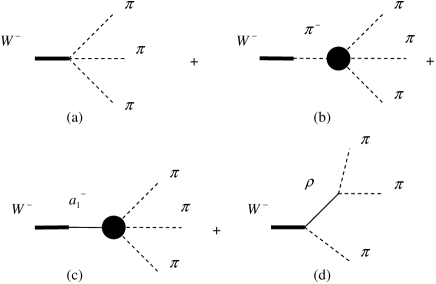
Figure 1: Diagrams schematically describing the transition $W^{-}\to\pi^{-}\pi^{-}\pi^{+}$. Shaded circles depict the transition including both the point-like and $\rho$-exchange contributions. Permutations of pion momenta are understood.

The amplitude of the decay $W^{-}(q)\to\pi^{+}(q_{1})\pi^{-}(q_{2})\pi^{-}(q_{3})$ corresponding to the diagrams Fig. 1 is

$$iM=\frac{g_{2}V_{ud}}{2f_{\pi}}\epsilon_{\mu}^{(W)}J_{\mu},$$ (20)

where $\epsilon_{\mu}^{(W)}$ is the polarization four-vector of $W^{-}$ boson and the axial decay current $J_{\mu}$ looks like

$$J_{\mu} = -q_{1\mu}+\frac{q_{\mu}}{D_{\pi}(q)}\left[m^{2}_{\pi}-(q,q_{1})+\frac{am^{2}_{\rho}}{2}\times\right.$$ (21)

$$\left.(1+\hat{P}_{23})\frac{(q_{2},q_{1}-q_{3})}{D_{\rho}(q_{1}+q_{3})}\right]-\frac{ar^{2}m^{2}_{a_{1}}}{2D_{a_{1}}(q)}\times$$

$$\left\{A_{1}q_{1\mu}+A_{2}q_{2\mu}+A_{3}q_{3\mu}-\frac{2q_{\mu}}{m^{2}_{a_{1}}}\times\right.$$

$$\left.(1+\hat{P}_{23})\left[(m^{2}_{\pi}+(q_{1},q_{2}))(q_{3},q_{1}-q_{2})\times\right.\right.$$

$$\left.\left.\left(\frac{\beta}{D_{\rho}(q_{1}+q_{2})}-\frac{r^{2}(\beta-1)}{m^{2}_{\rho}}\right)\right]\right\}+$$

$$\frac{am^{2}_{\rho}}{2}(1+\hat{P}_{23})\frac{(q_{1}-q_{3})_{\mu}}{D_{\rho}(q_{1}+q_{3})}.$$

In the above expressions, $D_{\rho}$, $D_{\pi}$, and $D_{a_{1}}$ are the inverse propagators of $\pi$, $\rho$, and $a_{1}$ mesons, respectively. Their expressions are given in Ref. ach05 . The terms corresponding to the diagrams (a), (b), (c), and (d) in Fig. 1 are easily identified by these propagators.

IV The spectrum of $\pi^{+}\pi^{-}\pi^{-}$ in $\tau^{-}\to\pi^{+}\pi^{-}\pi^{-}\nu_{\tau}$ decay

The spectrum of the three pion state in the decay $\tau^{-}\to\pi^{+}\pi^{-}\pi^{-}\nu_{\tau}$ normalized to its branching fraction is okun

$$\frac{dB}{ds} = \frac{(G_{F}V_{ud})^{2}(m^{2}_{\tau}-s)^{2}}{2\pi(2m_{\tau})^{3}\Gamma_{\tau}}\times$$ (22)

$$\left[(m^{2}_{\tau}+2s)\rho_{t}(s)+m^{2}_{\tau}\rho_{l}(s)\right],$$

$s=q^{2}$, $G_{F}$ is the Fermi constant, and $\Gamma_{\tau}$ is the width of $\tau$ lepton. The transverse and longitudinal spectral functions are, respectively,

$$\rho_{t}(s) = \frac{1}{3\pi sf^{2}_{\pi}}\int d\Phi_{3\pi}\left[\frac{|(q,J)|^{2}}{s}-(J,J^{\ast})\right],$$

$$\rho_{l}(s) = \frac{1}{\pi s^{2}f^{2}_{\pi}}\int d\Phi_{3\pi}|(q,J)|^{2},$$ (23)

where $d\Phi_{3\pi}$ is the element of Lorentz-invariant phase space volume of the system $\pi^{-}\pi^{-}\pi^{+}$.

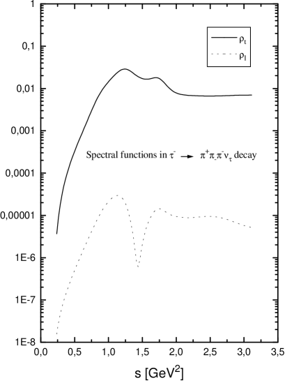
Figure 2: The transverse $\rho_{t}$ and longitudinal $\rho_{l}$ spectral functions in $\tau^{-}\to\pi^{+}\pi^{-}\pi^{-}\nu_{\tau}$ decay evaluated in GHLS model with the single axial vector meson under assumption of ”canonical” choice (1) of free parameters. See the text for more detail.

The numerical integration shows that $\rho_{l}$ is by about three orders of magnitude smaller than $\rho_{t}$ in all allowed kinematical range $9m^{2}_{\pi}<s<m^{2}_{\tau}$. See Fig. 2. By this reason it is neglected in what follows.

V Results

The ”canonical” choice (1) of free GHLS parameters bando88 with $m_{a_{1}}=1.23$ GeV results in the spectrum shown with the dot-dashed line in Fig. 3. It disagrees with the data both in lower branching ratio $B_{\tau^{-}\to\pi^{+}\pi^{-}\pi^{-}\nu_{\tau}}\approx 6\%$ and in the shape of the spectrum. Upon the variation of free parameters of the single $a_{1}$ resonance contribution listed in Eq. (1) one obtains the curve drawn in Fig. 3 with the dashed line. Corresponding parameters $m_{a_{1}}\approx 1.54\mbox{ GeV, }a\approx 1.75\mbox{, }r\approx 1.05\mbox{, }\beta\approx 0.84$ with $\chi^{2}/N_{\rm d.o.f.}=690/112$. reproduce the branching ratio $B_{\tau^{-}\to\pi^{+}\pi^{-}\pi^{-}\nu_{\tau}}\approx 9\%$ but the shape of the spectrum is not reproduced. Inclusion of additional higher derivative terms to the suggested in Refs. bando88a ; bando88 minimal set Eq. (1) and subjected to the fitting in the present work cannot improve the situation. Indeed, even the minimal set Eq. (1) results in a rather fast growth of the $a_{1}\to 3\pi$ decay width with the energy increase, see Ref. ach05 and Fig. 7 and 8 below in Sec. VI. Additional higher derivative terms would make the growth to be explosive. Restricting such a growth would require phenomenological form factors with free parameters. We believe that the dynamical explanation of the shape of the spectrum based on additional axial vector resonances $a_{1}^{\prime}$, $a_{1}^{\prime\prime}$ would be preferable. Note that there are indications on such resonances, both theoretical isgur87 ; isgur85 and experimental pdg ; amelin ; cleo .

Hence, to improve the fit, we include the contributions of heavier axial vector resonances $a_{1}^{\prime}$, $a_{1}^{\prime\prime}$. Taking them into account reduces to adding two diagrams similar to one in Fig. 1(c), with the replacement of $a_{1}(1260)$ by $a^{\prime}_{1}$ and $a^{\prime\prime}_{1}$. Since there is no available information concerning their couplings, the above resonances are included in a way analogous to $a_{1}(1260)$.

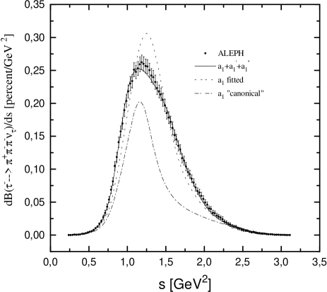
Figure 3: The spectrum of the decay $\pi^{+}\pi^{-}\pi^{-}$ state in $\tau$ normalized to the branching fraction $B_{\tau^{-}\to\pi^{-}\pi^{-}\pi^{+}\nu_{\tau}}$. The solid line is drawn for the set of GHLS parameters of the variant A of the Table 1. The ALEPH data are from Ref. aleph05 . See the text for more detail.

This prescription results in the amplitudes of the decays $a^{\prime}_{1},a^{\prime\prime}_{1}\to 3\pi$ vanishing when the four-momentum of any final pion vanishes. That is, the Adler condition is not violated upon adding the above resonances. In this sense the way of inclusion them respects chiral symmetry.

Figure 4: The spectrum of the decay $\pi^{+}\pi^{-}\pi^{-}$ in $\tau$ normalized to the branching fraction $B_{\tau^{-}\to\pi^{-}\pi^{-}\pi^{+}\nu_{\tau}}$. It corresponds to the variants C and D in the Table 2. The ALEPH data are from Ref. aleph05 . See the text for more detail.

The total set of the fitted parameters is first taken to be

$$(m_{a_{1}},a,r,\beta,m_{a^{\prime}_{1}},a^{\prime},r^{\prime},\beta^{\prime},w^{\prime},m_{a^{\prime\prime}_{1}},a^{\prime\prime},r^{\prime\prime},\beta^{\prime\prime},w^{\prime\prime}).$$

The parameters $a^{\prime}$, $r^{\prime}$, $\beta^{\prime}$ characterize the $a^{\prime}_{1}\to 3\pi$ decay amplitude similar to Eq. (16), (17) in the case of $a_{1}(1260)\to 3\pi$, while $w^{\prime}$ parameterizes the coupling $a^{\prime}_{1}\rho\pi$ as $g_{\rho\pi\pi}w^{\prime}r^{\prime}/f_{\pi}$. Compare with Eq. (16). Analogously for $a_{1}^{\prime\prime}$. The fit chooses $w^{\prime}=1$ and turns out to be insensitive to this parameter leaving $\chi^{2}/N_{\rm d.o.f}=122/102$. The quality of the fit can be considerably improved upon fixing $w^{\prime}=1$ but adding new parameter $\psi^{\prime}$-the phase of the $a^{\prime}_{1}$ contribution. Such phase imitates possible mixing among $a_{1}$, $a_{1}^{\prime}$, $a_{1}^{\prime\prime}$ resonances. The results of such type of the fit are given in the column variant A of the Table 1. Corresponding curve is shown in Fig. 3 with the solid line. Using Eqs. (12), (13), (14), (18), and obtaining $g_{\rho\pi\pi}=5.95$ from $\Gamma_{\rho\pi\pi}$ pdg one can compare the fitted GHLS parameters with the ”canonical” ones Eq. (1). To this end one should invoke the condition of cancelation Eq. (11) of the point-like $\gamma\pi^{+}\pi^{-}$ and $W^{-}\pi^{-}\pi^{0}$ vertices in GHLS. The relations expressing the original GHLS parameters through the fitted ones are the following:

$$b = r\left(\frac{m_{a_{1}}a}{2f_{\pi}g_{\rho\pi\pi}}\right)^{2},$$

$$c = (1-r)\left(\frac{m_{a_{1}}a}{2f_{\pi}g_{\rho\pi\pi}}\right)^{2},$$

$$d = \frac{a}{2}-r(1-r)\left(\frac{m_{a_{1}}a}{2f_{\pi}g_{\rho\pi\pi}}\right)^{2},$$

$$\alpha_{4} = 1-2\beta(1-r),$$

$$\alpha_{5} = \beta r,$$

$$\alpha_{6} = \alpha_{5}.$$ (24)

These GHLS parameters are marked in the Table 1 as ”calculated”. Since the basis of inclusion of heavier resonances $a_{1}^{\prime}$ and $a_{1}^{\prime\prime}$ here is purely phenomenological, specifically, there is no analog of gauge coupling constant $g$, we do not recalculate $(a^{\prime},b^{\prime},c^{\prime},d^{\prime},\cdots)$ and $(a^{\prime\prime},b^{\prime\prime},c^{\prime\prime},d^{\prime\prime},\cdots)$ similar to Eq. (24).

Table 1: The values of free parameters of GHLS model obtained from the unconstrained fit of the ALEPH data on the decay $\tau^{-}\to\pi^{+}\pi^{-}\pi^{-}\nu_{\tau}$ aleph05 (variant A), and the fit with the constrain $a=2$ preserving universality (variant B). Also shown are the corresponding calculated original bando88a ; bando88 GHLS parameters and the magnitudes of branching fractions of the above decay.

parameter	variant A	variant B
$m_{a_{1}}$[GeV]	$1.332\pm 0.015$	$1.139\pm 0.016$
$a$	$1.665\pm 0.011$	$\equiv 2$
$b$(calculated)	$1.35\pm 0.05$	$0.52\pm 0.03$
$c$(calculated)	$2.72\pm 0.08$	$3.74\pm 0.11$
$d$(calculated)	$-0.07\pm 0.03$	$0.54\pm 0.03$
$\alpha_{4}$(calculated)	$-10\pm 1$	$-27\pm 2$
$\alpha_{5}$(calculated)	$2.82\pm 0.06$	$1.94\pm 0.15$
$r$	$0.332\pm 0.007$	$0.122\pm 0.006$
$\beta$	$8.5\pm 0.3$	$15.9\pm 0.9$
$m_{a^{\prime}_{1}}$[GeV]	$1.59\pm 0.01$	$1.76\pm 0.01$
$a^{\prime}$	$0.99\pm 0.01$	$1.09\pm 0.01$
$r^{\prime}$	$0.96\pm 0.01$	$0.90\pm 0.01$
$\beta^{\prime}$	$0.07\pm 0.02$	$0.28\pm 0.02$
$w^{\prime}$	$\equiv 1$	$\equiv 1$
$\psi^{\prime}$	$28^{\circ}\pm 1^{\circ}$	$48^{\circ}\pm 1^{\circ}$
$m_{a^{\prime\prime}_{1}}$[GeV]	$1.88\pm 0.02$	$2.27\pm 0.02$
$a^{\prime\prime}$	$0.46\pm 0.01$	$0.59\pm 0.01$
$r^{\prime\prime}$	$1.45\pm 0.02$	$1.56\pm 0.02$
$\beta^{\prime\prime}$	$0.91\pm 0.05$	$0.91\pm 0.03$
$w^{\prime\prime}$	$1.14\pm 0.01$	$1.37\pm 0.01$
$\psi^{\prime\prime}$	$\equiv 0^{\circ}$	$\equiv 0^{\circ}$
$B_{\tau^{-}\to\pi^{+}\pi^{-}\pi^{-}\nu_{\tau}}$	$(9.05\pm 0.16)\%$	$(9.00\pm 0.15)\%$
$\chi^{2}/N_{\rm d.o.f}$	79/102	70/103

One can see that the obtained $a=1.665\pm 0.011$ is in disagreement with the universality condition $g_{\rho\pi\pi}=g$, which demands $a=2$, see Eq. (12). Hence we fulfill also the partially constrained fit with $a\equiv 2$, in order to preserve universality of the $\rho$ couplings. The results are presented as the variant B in the Table 1. Since the shape of the spectrum in the variant B is the same as in the Fig. 3, we do not show corresponding curve here.

Of a special interest is the width of the radiative decay $a_{1}^{\pm}\to\pi^{\pm}\gamma$. In order to evaluate the amplitude of this decay one should take into account the electromagnetic interaction. Upon neglecting the weak neutral current contribution, this is reduced to adding the terms

$$\bar{g}{\cal L}_{\mu}^{\rm e.m.}=eQ{\cal A}_{\mu},$$

$$\bar{g}{\cal R}_{\mu}^{\rm e.m.}=eQ{\cal A}_{\mu}$$

to the right hand side of the first and second lines of Eq. (8), respectively. Here, ${\cal A}_{\mu}$ stands for the field of the photon, $e$ is the elementary charge, and

$$Q=\frac{1}{3}\left(\begin{array}[]{cc}2&0\\ 0&-1\\ \end{array}\right)$$

is the charge matrix restricted to the sector of nonstrange mesons. As is known bando88a ; bando88 , the above decay originates from two sources. First, the $a_{1}\to\rho\pi$ transition followed by the transition $\rho\to\gamma$ which is given, upon neglecting the corrections to the masses of the second order in the electric charge, by the $\gamma\rho^{0}$ mixing term

$${\cal L}_{\gamma\rho}=-eagf^{2}_{\pi}\rho^{0}_{\mu}{\cal A}_{\mu}.$$ (25)

Second, one should add the direct $a_{1}\to\pi\gamma$ transition given by the term

$${\cal L}_{a_{1}\pi\gamma}=-iebf_{\pi}{\cal A}_{\mu}(a^{+}_{1\mu}\pi^{-}-a^{-}_{1\mu}\pi^{+}).$$ (26)

The resulting $a_{1}^{\pm}\to\pi^{\pm}\gamma$ decay width is represented in the form

$$\Gamma_{a^{\pm}_{1}\to\pi^{\pm}\gamma} = \frac{\alpha am^{3}_{a_{1}}}{24m^{2}_{\rho}}\left[r(\beta-1)\right]^{2}\left(1-\frac{m^{2}_{\pi}}{m^{2}_{a_{1}}}\right)^{3},$$ (27)

where $\alpha$ is the fine structure constant. Notice, that the above expression for $\Gamma_{a^{\pm}_{1}\to\pi^{\pm}\gamma}$ is written with the counter terms taken into account. The $a^{\pm}_{1}\to\pi^{\pm}\gamma$ decay amplitude without counter terms is proportional to the combination $b-arm^{2}_{a_{1}}/m^{2}_{\rho}$ which vanishes at any choice of GHLS parameters because of the relations (13), (14), and (18). The cancelation is due to the compensation of the diagram with the direct transition $a_{1}\to\pi^{\pm}\gamma$ expressed by the lagrangian Eq. (26) and one with the intermediate $\rho$ meson $a_{1}^{\pm}\to\rho^{0}\pi^{\pm}$ followed by the transition $\rho^{0}\to\gamma$, Eq. (25) bando88a ; bando88 .

The evaluation of $\Gamma_{a^{\pm}_{1}\to\pi^{\pm}\gamma}$ with the parameters from the variants A and B of the Table 1 gives the figures of the order of few MeV due to large values of $\beta$ in the Table 1 chosen by the fits. This is in disagreement with the measured ziel

$$\Gamma_{a^{\pm}_{1}\to\pi^{\pm}\gamma}=640\pm 246\mbox{ keV}.$$ (28)

Hence, one should further constrain the fit in order to incorporate the above radiative width. With the accuracy better than $4\%$ in $\Gamma_{a^{\pm}_{1}\to\pi^{\pm}\gamma}$ one can neglect the ratio $m^{2}_{\pi}/m^{2}_{a_{1}}$ and express the parameter $\beta$ as follows:

$$\beta=1+\frac{m_{\rho}}{rm_{a_{1}}}\left(\frac{24\Gamma_{a^{\pm}_{1}\to\pi^{\pm}\gamma}}{\alpha am_{a_{1}}}\right)^{1/2}.$$ (29)

When fitting, the central value of Eq. (28) is used. In addition, $a=2$ is kept fixed in order to provide the universality of the $\rho$ couplings.

It is found out that the fit with the fixed parameters $a$ and $\beta$ gives rather poor description with $\chi^{2}/N_{\rm d.o.f}=209/102$. The peculiar feature of the fit is that it chooses $\psi^{\prime}\approx 0$, the phase of the $a_{1}^{\prime}$ contribution, but $\chi^{2}$ is almost insensitive to the rather wide variations around above central value. Hence, we fix $\psi^{\prime}\equiv 0$, but introduce a new free parameter $\gamma$ whose meaning is $\gamma=m_{a_{1}}\Delta\Gamma_{a_{1}}$, where $\Delta\Gamma_{a_{1}}$ effectively takes into account the contributions to the $a_{1}$ resonance width other than $\rho\pi+3\pi\to 3\pi$ one, for example, $a_{1}\to\rho^{\prime}\pi\to 3\pi$, $K\bar{K}\pi$. They may be effective for the off-mass-shell $a_{1}$ meson. Of course, the approximation of the constant width for these contributions is oversimplified, but it nevertheless gives the rough estimate of their possible role as compared to the main contribution $a_{1}\to\rho\pi+3\pi\to 3\pi$ whose energy dependence is fully taken into account.

The results of the fit constrained by the conditions of the universality of the $\rho$ coupling and the fixed central value of $\Gamma_{a_{1}^{\pm}\to\pi^{\pm}\gamma}$ Eq. (28) are presented as the variant C in the Table 2. The spectrum of the system $\pi^{+}\pi^{-}\pi^{-}$ evaluated with the parameters of variant C is shown with the solid line in Fig. 4. Note that the found $\gamma=m_{a_{1}}\Delta\Gamma_{a_{1}}\sim 0.3$ GeV² corresponds to the portion of the $a_{1}$ decay channels different from $\rho\pi+3\pi\to 3\pi$ one, at the level $\Delta\Gamma_{a_{1}}/\Gamma_{a_{1}\to 3\pi}\sim 0.02$. This estimate can be obtained from the solid curve in Fig. 7 (or Fig. 8), where the calculated $\Gamma_{a_{1}\to\rho\pi+3\pi\to 3\pi}$ is shown. The above estimate demonstrates that the additional contribution to the $a_{1}$ width beside the GHLS one is very small.

Further evaluation shows that the contribution of the resonance $a_{1}^{\prime\prime}$, see Fig. 6 and sec. VI below, is rather small. Hence, we fulfill the fit in which the contribution of the resonance is absent. The parameters found in such type of the fit are listed in the the column variant D of the Table 2. The branching ratio $B_{\tau^{-}\to\pi^{+}\pi^{-}\pi^{-}\nu_{\tau}}$ and the visual shape of the spectrum in the variant D are in reasonable agreement with the data, but the magnitude of $\chi^{2}/N_{\rm d.o.f}$ is larger by the factor of two as compared to the variant C. This description is achieved with rather large phase of the $a_{1}^{\prime}$ contribution $\psi^{\prime}\approx 40^{\circ}$ pointing to a rather strong $a_{1}a_{1}^{\prime}$ mixing in the considered variant D. The curve corresponding to the variant D is shown in Fig. 4 with the dot-dash line.

Table 2: The values of free parameters of GHLS model obtained from the fit of the ALEPH data on the decay $\tau^{-}\to\pi^{+}\pi^{-}\pi^{-}\nu_{\tau}$ aleph05 constrained in a way as to fix $a\equiv 2$ and $\Gamma_{a_{1}^{\pm}\to\pi^{\pm}\gamma}$ (28). Variant C is the fit including $a_{1}+a_{1}^{\prime}+a_{1}^{\prime\prime}$ contributions. Variant D includes only $a_{1}+a_{1}^{\prime}$ ones. Also shown are the corresponding calculated original bando88a ; bando88 GHLS parameters and the magnitudes of branching fractions of the above decay.

parameter	variant C	variant D
$m_{a_{1}}$[GeV]	$1.368\pm 0.006$	$1.401\pm 0.006$
$a$	$\equiv 2$	$\equiv 2$
$b$(calculated)	$4.89\pm 0.07$	$5.37\pm 0.06$
$c$(calculated)	$1.30\pm 0.07$	$1.12\pm 0.05$
$d$(calculated)	$-0.03\pm 0.06$	$0.07\pm 0.04$
$\alpha_{4}$(calculated)	$0.66\pm 0.06$	$0.45\pm 0.05$
$\alpha_{5}$(calculated)	$1.29\pm 0.10$	$1.31\pm 0.10$
$r$	$0.790\pm 0.008$	$0.827\pm 0.006$
$\beta$(calculated)	$1.63\pm 0.12$	$1.58\pm 0.12$
$\gamma$[GeV2]	$0.31\pm 0.01$	$0.35\pm 0.02$
$m_{a^{\prime}_{1}}$[GeV]	$1.422\pm 0.007$	$1.513\pm 0.001$
$a^{\prime}$	$1.80\pm 0.03$	$2.01\pm 0.03$
$r^{\prime}$	$0.386\pm 0.005$	$0.370\pm 0.006$
$\beta^{\prime}$	$0.96\pm 0.05$	$0.82\pm 0.05$
$w^{\prime}$	$1.19\pm 0.01$	$1.18\pm 0.02$
$\psi^{\prime}$	$\equiv 0$	$39^{\circ}\pm 1^{\circ}$
$m_{a^{\prime\prime}_{1}}$[GeV]	$1.800\pm 0.007$	$-$
$a^{\prime\prime}$	$-0.32\pm 0.02$	$-$
$r^{\prime\prime}$	$0.36\pm 0.02$	$-$
$\beta^{\prime\prime}$	$-0.2\pm 0.2$	$-$
$w^{\prime\prime}$	$0.30\pm 0.04$	$-$
$\psi^{\prime\prime}$	$10^{\circ}\pm 8^{\circ}$	$-$
$B_{\tau^{-}\to\pi^{+}\pi^{-}\pi^{-}\nu_{\tau}}$	$(8.97\pm 0.13)\%$	$(8.96\pm 0.17)\%$
$\chi^{2}/N_{\rm d.o.f}$	45/102	95/107

At last, for the sake of completeness, we give the results of the fit of the data with the single $a_{1}$ resonance in the variant with $a\equiv 2$ and $\beta$ fixed from the radiative width. The fit is rather poor. To be specific, one obtains $m_{a_{1}}=1.685\pm 0.006$ GeV, $r=0.973\pm 0.005$, $\gamma=0.51\pm 0.02$ GeV², and $\chi^{2}/N_{\rm d.o.f}=389/113$. The corresponding spectrum is shown in Fig. 4 with the dotted line.

VI Discussion and conclusion

The simplest variant of the generalized hidden local symmetry model with the minimal set of the counter terms in its application to the $\tau^{-}\to\pi^{+}\pi^{-}\pi^{-}\nu_{\tau}$ decay is considered in the present work. This set simultaneously solves the problem of cancelation of the strong momentum dependence of the $\rho\pi\pi$ vertex and provides the measured value of the $a_{1}^{\pm}\to\pi^{\pm}\gamma$ decay width bando88a ; bando88 . It is shown that the variant with the single axial vector meson $a_{1}(1260)$ and with the above minimal set of free GHLS parameters meets troubles when describing the shape of the spectrum $\pi^{+}\pi^{-}\pi^{-}$. No reasonable fit can reproduce the shape, although the branching ratio $B_{\tau^{-}\to\pi^{+}\pi^{-}\pi^{-}\nu_{\tau}}$ agrees with the experiment.

Figure 5: Contributions to the spectrum of $\pi^{+}\pi^{-}\pi^{-}$ in $\tau$ decay in the variant A of the Table 1. The dashed line corresponds to the sum of the diagrams Fig. 1. See the text for more detail.

Figure 6: Contributions to the spectrum of $\pi^{+}\pi^{-}\pi^{-}$ in $\tau$ decay in the variant C of the Table 2. The dashed line corresponds to the sum of the diagrams Fig. 1. See the text for more detail.

One can hardly hope that higher derivatives or/and chiral loops may improve the apparently resonant behavior. The chiral loop contributions (besides the finite width ones) were shown to be of little importance in the four pion channel ecker , and one cannot expect they may help in the three pion axial vector channel, too. As for the higher derivative contributions, there exist the extensions li of GHLS chiral model with additional higher derivative terms besides the minimal set proposed in Ref. bando88a ; bando88 . In fact, no one so far has exhausted a full list of all possible higher derivative terms of the GHLS model. But, as we point out in first paragraph of the preceding section, any of such higher derivative term would demand the introduction of the phenomenological form factor restricting inevitable explosive growth of the partial width with the energy increase. This statement applies to the terms suggested in Ref. li as well.

We believe that more natural is the inclusion of the contributions of heavier axial vector mesons, in order to reconcile calculations in GHLS with the minimal set of counter terms bando88a ; bando88 with available data aleph05 . Like the vector resonances $\rho^{\prime}$, $\rho^{\prime\prime}$ pdg , the existence of above resonances is naturally expected in the both quark model and large $N_{c}$ expansion. Experiment pdg ; amelin ; cleo gives the evidence in favor of such resonances, too. The results of the present study show that contributions of the heavier axial vector resonances $a^{\prime}_{1}$ and $a^{\prime\prime}_{1}$ added to the $a_{1}(1260)$ one are capable of reproducing both the branching ratio and the correct shape of the pion spectrum in the decay $\tau^{-}\to\pi^{+}\pi^{-}\pi^{-}\nu_{\tau}$.

We would like to remind that similar problem with the simplest ”canonical” GHLS model was found in the vector channel $e^{+}e^{-}\to\pi^{+}\pi^{-}\pi^{+}\pi^{-}$ considered earlier ach08a ; ach08b . The analysis presented in the above works shows that the contributions of heavier resonances $\rho^{\prime}$ and $\rho^{\prime\prime}$ are required for correct description of experimental data at energy $\sqrt{s}\approx 1$ GeV. However, contrary to the case of the vector channel where additional contributions of $\rho^{\prime}$ and $\rho^{\prime\prime}$ at the above energy exceed the $\rho(770)$ one, in the axial vector channel considered in the present work, each of the additional contributions is smaller in magnitude than the contribution of pure GHLS with the single fitted $a_{1}$ resonance. See Fig. 5 and 6. But they contribute almost coherently resulting in the acceptable shape of the spectrum and the acceptable magnitude of the branching fraction $B(\tau^{-}\to\pi^{+}\pi^{-}\pi^{-}\nu_{\tau})\approx 9\%$. Specifically, with the central values of the fitted parameters of the variants A in the Table 1 (the variants C in the Table 2), respectively, one obtains for the net contribution of the diagrams Fig. 1(a), (b), (c), and (d) the branching fraction $B(\tau^{-}\to\pi^{+}\pi^{-}\pi^{-}\nu_{\tau})\approx 2.65(6.21)\%$. The contribution of the diagram Fig. 1(c) amounts to $B(\tau^{-}\to\pi^{+}\pi^{-}\pi^{-}\nu_{\tau})\approx 0.33(2.1)\%$. These figures should be compared with the contributions of the diagram Fig. 1(c) in which $a_{1}$ is replaced by $a^{\prime}_{1}$ and $a^{\prime\prime}_{1}$. One obtains $B(\tau^{-}\to\pi^{+}\pi^{-}\pi^{-}\nu_{\tau})\approx 1.15(0.51)\%$ and $0.67(0.01)\%$, respectively.

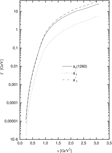
Figure 7: The widths of decay into $3\pi$ of the resonances $a_{1}(1260)$, $a_{1}^{\prime}$, and $a_{1}^{\prime\prime}$ evaluated with the fitted parameters of the variant A in the Table 1.

It is worth noting that in the variant A of the Table 1 the visible $a^{\prime\prime}_{1}$ peak position is lower than that of $a^{\prime}_{1}$ despite of the fact that their bare masses are in opposite relation, see the Table 1. This can be explained as follows. Here the dominant decay mode of $a_{1}^{\prime}$, $a_{1}^{\prime\prime}$ resonances is the $3\pi$ one. Its partial width grows rapidly with energy increase reaching the figures compatible with bare mass itself. As was pointed out earlier ach00a , the combined action of the strong energy dependence of the partial width and its large magnitude shifts the visible peak towards the lower energies. The more the width and the more its growth, the more the peak shifts. Since the width of the resonance $a_{1}^{\prime\prime}$ and its growth are stronger as compared to $a_{1}^{\prime}$, see Fig. 7 for the variant A of the Table 1, its visible position appears at lower energy than the visible position of $a_{1}^{\prime}$. For comparison, the three pion decay widths of the resonances $a_{1}$, $a_{1}^{\prime}$, and $a_{1}^{\prime\prime}$ evaluated with the parameters of the variant C of the Table 2 are shown in Fig. 8.

Figure 8: The widths of decay into $3\pi$ of the resonances $a_{1}(1260)$, $a_{1}^{\prime}$, and $a_{1}^{\prime\prime}$ evaluated with the fitted parameters of the variant C in the Table 2.

In principle, the vector isovector resonances $\rho^{\prime}$, $\rho^{\prime\prime}$ could be present in the final states of the present axial vector isovector channel $\pi^{+}\pi^{-}\pi^{-}$, via the transition $a_{1}\to\rho^{\prime}(\rho^{\prime\prime})\pi\to 3\pi$ (analogously for $a^{\prime}_{1}$, $a^{\prime\prime}_{1}$). However, their inclusion requires the introduction of new free parameters $g_{a_{1}\rho^{\prime}(\rho^{\prime\prime})\pi}$ (analogously for $a^{\prime}_{1}$, $a^{\prime\prime}_{1}$) in addition to those 14 ones already present. On the grounds of reasonable adequacy we neglect $\rho^{\prime}$, $\rho^{\prime\prime}$ at the present stage of the study, especially because the coupling constants $g_{\rho^{\prime}\pi\pi}$ and $g_{\rho^{\prime\prime}\pi\pi}$ are presumably small as compared to $g_{\rho\pi\pi}$ ach97 .

We would like to thank M. Davier for providing us the reference to the ALEPH data in the table form. The present work is supported in part by Russian Foundation for Basic Research grant RFFI-10-02-00016.

References

(1)
M. Bando, T. Kugo, S. Uehara et al., Phys.Rev.Lett. 54,
1215 (1985).
(2)
M. Bando, T. Fujiwara, and K. Yamawaki, Progr.Theor.Phys. 79,
1140 (1988).
(3)
M. Bando, T. Kugo, and K. Yamawaki, Phys.Rept. 164, 217
(1988). See also review meissner88 .
(4)
Ulf-G. Meissner, Phys.Rept. 161, 213 (1988).
(5)
Ö. Kaymakcalan, S. Rajeev, and. J. Schechter, Phys.Rev.D30, 594 (1984).
(6)
N. N. Achasov and A. A. Kozhevnikov, Phys.Rev.D71, 034015
(2005)[arXiv:hep-ph/0412077v2]; Yad.Fiz.69, 314 (2006)
[Phys.Atom.Nucl.69, 293 (2006)].
(7)
N. N. Achasov and A. A. Kozhevnikov, Pisma v ZhETF 88, 3
(2008) [JETP Lett.88, 1 (2008)]; [arXiv:0803.2972v2].
(8)
N. N. Achasov and A. A. Kozhevnikov, Eur.Phys.J.A38, 61
(2008) [arXiv:0809.3883v1].
(9)
R. R. Akhmetshin, et al. (CMD-2 Collab.), Phys.Lett.
B475, 190 (2000) [arXiv:hep-ex/9912020v1].
(10)
B. Aubert, et al. (BaBaR Collab.), Phys.Rev. D71,
052001 (2005) [arXiv:hep-ex/0502025v1].
(11)
S. Schael et al. (ALEPH Collaboration), Phys.Rept.421,
191 (2005).
(12)
D. Gómez Dumm, A. Pich, and J. Portolés, Phys. Rev. D69, 073002 (2004)[arXiv:hep-ph/0312183].
(13)
D. Gómez Dumm, P. Roig, A. Pich, and J. Portolés
[arXiv:0911.4436v1]
(14)
M. Vojik and P. Lichard [arXiv:1006.2919].
(15)
S. L. Adler, Phys.Rev.139, B1638 (1965).
(16)
L. B. Okun’, Leptons and Quarks, Nauka Publishers, Moscow
(1990).
(17)
R. Kokoski and N. Isgur, Phys.Rev.D35, 907 (1987).
(18)
S. Godfrey and N. Isgur, Phys.Rev.D32, 189 (1985).
(19)
K. Nakamura et al. (Particle Data Group), J. Phys. G 37, 075021 (2010)
(20)
D. V. Amelin, et al., (the VES Collaboration), Phys. Lett.
B356, 595 (1995).
(21)
D. Asner, et al. (CLEO Collaboration), Phys.Rev.D61,
012002(2000) [arXiv:hep-ex/9902022v1].
(22)
M. Zielinski et al., Phys.Rev.Lett. 52, 1195 (1984).
(23)
G. Ecker and R. Unterdorfer, Eur.Phys.Journal C24, 535 (2002) [arXiv:hep-ph/0203075v2].
(24)
Bing An Li and Yue-Liang Wu, Mod.Phys.Lett.A22, 683(2007) [arXiv:hep-ph/0509054].
(25)
N. N. Achasov and A. A. Kozhevnikov, Phys.Rev.D62,117503(2000) [arXiv:hep-ph/0007205v2];
Yad.Fiz.65,158(2002) [Phys.Atom.Nucl.65153(2002)].
(26)
N. N. Achasov and A. A. Kozhevnikov, Phys.Rev.D55, 2663
(1997)[arXiv:hep-ph/9609216v1].