Recurrences in three-state quantum walks on a plane

Abstract

We analyze the role of dimensionality in the time evolution of discrete time quantum walks through the example of the three-state walk on a two-dimensional, triangular lattice. We show that the three-state Grover walk does not lead to trapping (localization) or recurrence to the origin, in sharp contrast to the Grover walk on the two dimensional square lattice. We determine the power law scaling of the probability at the origin with the method of stationary phase. We prove that only a special subclass of coin operators can lead to recurrence and there are no coins leading to localization. The propagation for the recurrent subclass of coins is quasi one-dimensional.

I Introduction

The speed of propagation is affected critically by the spatial dimensions in diverse systems, ranging from classical statistical phenomena like diffusion or percolation percolation ; odor to various quantum transport effects nazarov . One of the simplest models capturing the essence of classical diffusive propagation is a random walk on a regular lattice revesz . The sensitivity of a random walk to the number of spatial dimensions is clearly shown by its recurrence properties. A balanced random walker on a regular square lattice returns to its starting point with certainty in dimensions 1 and 2 if we wait long enough, whereas there is a nonzero probability of escape in dimension 3 or higher, as discovered by Pólya polya . The probability to return to the origin is now called the Pólya number.

The generalization of the discrete time random walk to a quantum walk was first introduced by Aharonov, Davidovich and Zagury aharonov_1993 , and independently, from a quantum information theoretical perspective, by Meyer meyer . In the past few years, there has been a considerable number of studies devoted to quantum walks santha_2008 , strongly motivated by their possible application for designing quantum algorithms kendon_2006 . In discrete time walks the external, position degrees of freedom are assisted by a finite number of internal degrees of freedom, the chirality or coin. The situation resembles to the discrete version of the Chalker-Coddington model chalker-coddington . Recent experimental demonstration of discrete-time quantum walks with many steps in different physical systems (trapped ions zahringer , optically trapped atoms karski , linear quantum optics schreiber_2010 ) pave the way to study more complex behavior of quantum walks in the laboratory.

In quantum walks, the question of finding the walker involves the measurement of its position. The measurement unavoidably disturbs the quantum system, which has to be taken into account when defining quantities to describe its spreading, like the hitting time hittingreview . We have defined the generalized Pólya number stefanak_prl_2008 to characterize the probability of return to the origin of a quantum walker starting from a localized position. In order to minimize the disturbance we have adopted a scheme for measurements, where each system from an ensemble is observed only once kiss-kecskes . The quantum Pólya number exhibits strikingly different behaviour compared to its classical counterpart. In dimension 2, the symmetric quantum walk on a square lattice can be recurrent (Pólya number 1) or transient (Pólya number less than 1) depending on the coin operator and the initial state stefanak_pra_2008 . For certain coins, localization (trapping) at the origin can occur localization . In dimension 1, although both classical and quantum unbiased walks have a Pólya number 1, classically the effect is unstable towards the introduction of a bias while in the quantum case there is a region of stability stefanak_njp_2009 . These results indicate that the recurrence of walks is not only sensitive to the dimension of the underlying lattice, but in the quantum case also the coin degree of freedom can ultimately determine its behaviour. In the one dimensional case, one can increase the dimension of the coin space from 2 to 3, by allowing the walker to stay at its position leading to localization inui_2005 . Further increasing the dimension of the coin space can possibly introduce more interesting effects inui_2003 .

The triangular lattice is a planar graph with symmetry properties different from the square lattice. It can define either a rank 3 oriented graph or a rank 6 undirected graph. Quantum walks on triangular lattices have been considered for designing effective quantum algorithms abal_arxiv_2010 . Discrete-time quantum walks, especially on triangular lattices, provide a platform to realize topological phases kitagawa . Propagation of continuous-time quantum walks have also been recently studied in jafarizadeh .

In this paper, we consider a two dimensional walk on an oriented triangular graph with a three-state coin space. The classical symmetric random walk on such a graph is recurrent, similar to the two-dimensional square lattice. We analyze the quantum walk on this lattice and prove that neither localization nor recurrence is possible for any unbiased coin, except for trivial cases. We calculate the asymptotic decay of the probability at the origin for the Grover coin and discuss its dependence on the initial state.

The paper is organized as follows. In Section II. we introduce the three-state quantum walk on the triangular lattice and describe the asymptotic behavior of such a quantum walk with the help of the method of stationary phase. In Section III. we analyze the recurrence properties of the walk driven by the Grover matrix. We dedicate Section IV. to find the general requirements of the recurrence in arbitrary coin matrices, we prove that only a special subclass of coins leads to recurrence, we demonstrate the quasi-onedimensional propagation leading to recurrence of such walks by constructing an example. We summarize our results in Section V. For the sake of completeness we show the recurrence properties of the classical walk on the triangular lattice in Appendix A.

II Description of the three-state quantum walks

The Hilbert space of the three-state quantum walk on the $2$-dimensional lattice has the tensor product structure

$$\mathcal{H}=\mathcal{H}_{P}\otimes\mathcal{H}_{C}\,,$$ (1)

where $\mathcal{H}_{P}$ denotes the so-called position-space spanned by the vectors $|\textbf{m}\rangle$ corresponding to the walker being at the lattice point m

$$\mathcal{H}_{P}={\rm Span}\left\{|\textbf{m}\rangle\,|\,\,\textbf{m}\in\mathds{Z}^{2}\right\}=\ell^{2}(\mathds{C}^{2})\,.$$ (2)

The three-dimensional coin-space $\mathcal{H}_{C}$ has the structure

$$\mathcal{H}_{C}=\text{Span}\left\{|\mathbf{e}_{i}\rangle\,|\,\,i=1,2,3\right\}\,,$$ (3)

where the coin state (chirality) $|\mathbf{e}_{i}\rangle$ corresponds to the displacement of the particle by $\mathbf{e}_{i}$, a two dimensional vector on the plane of walk. The triangle-like topology of the walk (see Figure 1) leads to the following form of the displacement vectors

$$\mathbf{e}_{1}=(-\frac{1}{2},\frac{\sqrt{3}}{2}),\quad\mathbf{e}_{2}=(1,0),\quad\mathbf{e}_{3}=(-\frac{1}{2},-\frac{\sqrt{3}}{2})\,.$$ (4)

The walks in consideration are unbiased in a sense, that

$$\sum_{i=1}^{3}{\mathbf{e}_{i}}=0\,.$$ (5)

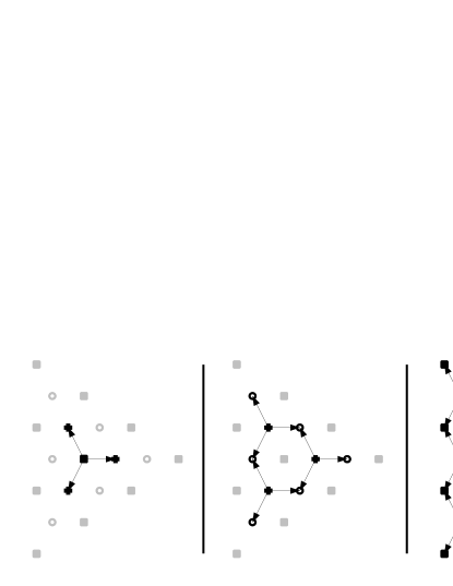
Figure 1: The lattice points which the walker starting from the origin (central vertex) can reach in 3 steps, with the available displacement vectors.

A single step of the quantum walk is given by the propagator

$$U=S\cdot(I_{P}\otimes C)\,.$$ (6)

Here $I_{P}$ denotes the identity operator on $\mathcal{H}_{P}$. The operator $C$ represents the coin flip and acts only on $\mathcal{H}_{C}$. The conditional step operator $S$ is responsible for the actual displacement of the walker from position m to $\textbf{m}+\mathbf{e}_{i}$ with respect to the coin state $|\mathbf{e}_{i}\rangle$ and has the following form

$$S=\sum_{\mathbf{m}}\sum_{i=1}^{3}{|\textbf{m}+\mathbf{e}_{i}\rangle\langle\textbf{m}|\otimes|\mathbf{e}_{i}\rangle\langle\mathbf{e}_{i}|}\,.$$ (7)

The state of the walker after $t$ time steps is given by the application of the time evolution operator (6) on the initial state

$$|\psi(t)\rangle\equiv\sum_{\textbf{m},i}\psi_{i}(\textbf{m},t)|\mathbf{m}\rangle\otimes|\mathbf{e}_{i}\rangle=U^{t}|\psi(0)\rangle\,.$$ (8)

The probability of finding the walker at the lattice point m at time $t$ is given by the summation over the coin states

$$p(\textbf{m},t) \equiv \sum_{i=1}^{3}|\langle\textbf{m}|\otimes\langle\mathbf{e}_{i}|\psi(\textbf{m},t)\rangle|^{2}=\sum_{i=1}^{3}|\psi(\textbf{m},t)|^{2}$$ (9)

$$= ||\psi(\textbf{m},t)||^{2},$$

Here, we have introduced the vector of probability amplitudes at the lattice point $\mathbf{m}$

$$\psi(\textbf{m},t)\equiv(\psi_{1}(\textbf{m},t),\psi_{2}(\textbf{m},t),\psi_{3}(\textbf{m},t))^{T}\,.$$ (10)

Since we focus on the recurrence properties of the three-state quantum walks we consider initial states according to the classical Pólya problem, i.e. the walker starts localized at the origin. Hence, the probability amplitudes vanishes except at the origin

$$\psi_{i}(\textbf{m},0)=0,\quad\mathbf{m}\neq\mathbf{0}\,.$$ (11)

Nevertheless, we have the freedom to choose the initial orientation of the coin which we denote by the vector of probability amplitudes $\psi=\left(\psi_{1}(\textbf{0},0),\psi_{2}(\textbf{0},0),\psi_{3}(\textbf{0},0)\right)^{T}.$

Since the three-state quantum walk is translationally invariant the time evolution equation (8) is greatly simplified by the Fourier transformation

$$\tilde{\psi}(\textbf{k},t)\equiv\sum_{\textbf{m}}\psi(\textbf{m},t)e^{i\textbf{k}\cdot\textbf{m}},\qquad\textbf{k}\in\mathds{K}^{2}\,,$$ (12)

where $\mathds{K}=(-\pi,\pi]$. The time evolution in the Fourier picture simplifies into a single difference equation

$$\tilde{\psi}(\textbf{k},t)=\tilde{U}^{t}(\textbf{k})\tilde{\psi}(\textbf{k},0)=\tilde{U}^{t}(\textbf{k})\psi\,.$$ (13)

where $\tilde{\psi}(\textbf{k},0)$ denotes the Fourier transformation of the initial state. The propagator in the Fourier picture $\tilde{U}$ is given by

$$\tilde{U}=D(\textbf{k})\cdot C\,,$$ (14)

where $D(\textbf{k})$ is a diagonal matrix determined by the displacement vectors $\mathbf{e}_{i}$

$$D(\textbf{k})=\mathrm{Diag}\left(e^{-i\textbf{k}\cdot\mathbf{e}_{1}},e^{-i\textbf{k}\cdot\mathbf{e}_{2}},e^{-i\textbf{k}\cdot\mathbf{e}_{3}}\right)\,.$$ (15)

The time evolution equation in the Fourier picture (13) is readily solved by diagonalizing the propagator $\tilde{U}$. Since $\tilde{U}$ is an unitary matrix its eigenvalues have the form

$$\lambda_{j}(\textbf{k})=e^{i\omega_{j}(\textbf{k})}\,.$$ (16)

The solution in the position representation reads

$$\psi(\textbf{m},t)=\sum_{j=1}^{3}\int_{\mathds{K}^{2}}\frac{d\textbf{k}}{(2\pi)^{2}}e^{-i\textbf{k}\cdot\textbf{m}}e^{i\omega_{j}(\textbf{k})t}\left(v_{j}(\textbf{k}),\psi\right)v_{j}(\mathbf{k})\,.$$ (17)

We concentrate on the recurrence nature of the quantum walks which is determined by the asymptotic behaviour of the probability at the origin. This can be readily analyzed by means of the method of stationary phase. Indeed, the amplitude at the origin reads

$$\psi(\textbf{0},t)=\sum_{j=1}^{3}\int_{\mathds{K}^{2}}\frac{d\textbf{k}}{(2\pi)^{2}}e^{i\omega_{j}(\textbf{k})t}\left(v_{j}(\textbf{k}),\psi\right)v_{j}(\mathbf{k})\,,$$ (18)

and the probability is simply the absolute square of the amplitude. Within the stationary phase approximation the important points in the integration domain are those where the phase $\omega_{j}(\textbf{k})$ has a vanishing derivative, i.e. stationary points. The rate at which the integrals in (18) decay is determined by the flatness of the phase at the stationary points. For a two-dimensional walk with a finite number of non-degenerate saddle points the probability amplitude at the origin decays as $t^{-1}$, with the probability decaying as $t^{-2}$ leading to a transient walk. A continuum of saddle points (saddle line) leads to a probability amplitude decaying at a rate $t^{-1/2}$, the probability decays as $t^{-1}$ at the origin, thus resulting in recurrence.

III Grover walk

The Grover operator plays a key role in Grover’s search algorithm. Used as a coin operator for regular two-dimensional quantum walks on a Cartesian lattice it leads to the phenomenon of localization for all initial coin states except one well defined state. Moreover it is widely used in quantum walk based search algorithms.

The Grover matrix is an orthogonal matrix with elements defined as

$$G^{(d)}_{i,j}=\frac{2}{d}-\delta_{i,j}\,.$$ (19)

This matrix has an important symmetry. Indeed, it commutes with all permutation matrices. Hence, in the $d=3$ case cyclic permutation of the initial chiralities will only rotate the probability distribution by $2\pi/3$ in the positive or the negative direction. To obtain a rotationally invariant probability distribution we have to choose an initial state which is invariant under cyclic permutations. Since the global phase of the quantum state is irrelevant we find such a symmetric probability distribution results from the initial coin state

$$\psi_{S}=\frac{1}{\sqrt{3}}\left(1,1,1\right)^{T}\,.$$ (20)

Moreover, the symmetry of the Grover operator implies that permuting the initial chiralities does not change the recurrence properties of the Grover walk.

Let us analyze the recurrence of the three-state Grover walk in more detail. For that purpose we have to find the asymptotic behaviour of the probability at the origin. This is determined by the stationary points of the eigenenergies $\omega_{j}(\mathbf{k})$ of the propagator $\tilde{U}(\mathbf{k})$ in the Fourier picture. For the Grover walk the eigenenergies are given by the implicit function

$$\Phi(\omega,\mathbf{k}) = \det\left(\tilde{U}(\mathbf{k})-e^{i\omega}I\right)=$$

$$= \sin\left(k_{1}-\frac{\omega}{2}\right)-2\cos\left(\frac{\sqrt{3}k_{2}}{2}\right)\sin\left(\frac{k_{1}+\omega}{2}\right)-$$

$$- 3\sin\left(\frac{3\omega}{2}\right)=0\,.$$

It is straightforward to show by implicit differentiation that the stationary point is $\mathbf{k}_{0}=\mathbf{0}$. Moreover, also the second derivatives are vanishing at $\mathbf{k}_{0}$. To clarify this statement, we consider the eigenvalues of $\tilde{U}(\mathbf{k})$ for $k_{1}=0$ or $k_{2}=\frac{1}{\sqrt{3}}k_{1}$. In both cases we find that one eigenvalue, say $\lambda_{1}$, is constant and equals unity, i.e.

$$\omega_{1}(k_{1}=0,k_{2})=\omega_{1}(k_{1},k_{2}=\frac{1}{\sqrt{3}}k_{1})=0\,.$$ (22)

Hence, all derivatives of $\omega_{1}$ with respect to $k_{1}$ at the line $k_{2}=\frac{1}{\sqrt{3}}k_{1}$ vanish, the same applies on the line $k_{1}=0$ with taking the derivatives with respect to $k_{2}$. Therefore, the second derivatives of $\omega_{1}(\mathbf{k})$ vanish at the stationary point $\mathbf{k}_{0}=\mathbf{0}$, i.e. the rank of the Hessian matrix at $\mathbf{k}$ is zero. In such a case, the method of stationary phase indicates that the integrals in the probability amplitude (18) decay like $t^{-2/3}$ as $t$ approaches infinity. Hence, the decay of the probability at the origin is given by $p_{0}(t)\sim t^{-4/3}$ which is faster than the threshold required for the recurrence. We conclude that the three-state Grover walk on a plane is transient, i.e. its Pólya number is less than unity.

The decay of the probability at the origin can be even faster than what we have already found. Indeed, we can eliminate the stationary point $\mathbf{k}_{0}$ by the proper choice of the initial coin state $\psi$. Such $\psi$ has to be orthogonal to the eigenvector corresponding to $\lambda_{1}$ at the stationary point $\mathbf{k}_{0}$, which is easily found to be

$$v_{1}(\mathbf{k}_{0})=\frac{1}{\sqrt{3}}\left(1,1,1\right)^{T}\,.$$ (23)

Hence, the initial coin state has to be of the form

$$\psi_{G}=\left(a,b,c\right)^{T},\quad a+b+c=0\,.$$ (24)

Starting the three-state Grover walk with an initial state from the subspace (24) will lead to fast decay of the probability at the origin.

We illustrate these results in Figures 2 and 3. In Figure 2 we choose the initial state $\psi_{S}$ of (20). The resulting probability distribution shown in the upper plot is symmetric and peaked at the origin. However, in contrast to the Grover walk on a Cartesian lattice, the current model does not exhibit localization. In the lower plot, $p_{0}(t)$ is shown on a double logarithmic scale. The numerical results agree with the power law $p_{0}(t)\sim t^{-4/3}$ predicted by the method of stationary phase.

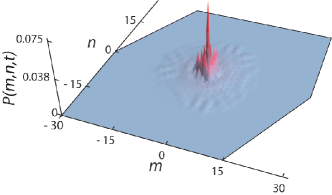
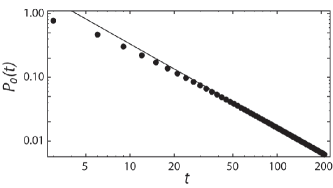
Figure 2: (Color online) Probability distribution of the three-state Grover walk on a plane and the time dependence of the probability at the origin (throughout the paper time $t$ is measured in dimensionless units, corresponding to one step). In the upper plot we display the probability distribution after 30 steps. The initial coin state was chosen to be $\psi_{S}=\frac{1}{\sqrt{3}}\left(1,1,1\right)^{T}$. We find that the probability distribution is symmetric and peaked at the origin. However, the probability at the origin is decaying according to a power law. The lower plot is in loglog scale to unravel the scaling law on a longer time scale. The straight line corresponds to $t^{-4/3}$.

In Figure 3, the initial state was chosen to be $\psi=\frac{1}{\sqrt{3}}\left(1,e^{i2\pi/3},e^{i4\pi/3}\right)^{T}$ which belongs to the subspace (24). The peak of the probability distribution at the origin vanishes (upper plot). The numerical results of the probability at the origin presented in the lower plot indicate that the decay rate has doubled to $p_{0}(t)\sim t^{-8/3}$.

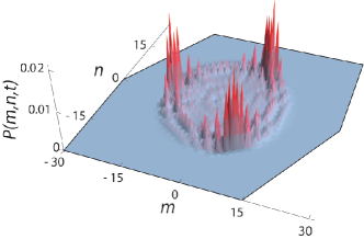
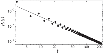
Figure 3: (Color online) Probability distribution of the three-state Grover walk on a plane and the time dependence of the probability at the origin for the initial state $\psi=\frac{1}{\sqrt{3}}\left(1,\exp({i2\pi/3}),\exp({i4\pi/3})\right)^{T}$. Since $\psi$ belongs to the family (24) the behaviour of the Grover walk is changed considerably. The peak at the origin has vanished, as illustrated in the upper plot. Most of the probability is located on the ring. Moreover, the decay of the probability at the origin is faster when compared to the power law we have found for the initial states outside of the subspace (24) . On the lower plot we show the long time behaviour of the probability at the origin, thus indicating that the exponent of the power law has doubled to $-8/3$. We use a loglog scale to make the power law more visible. The straight line corresponds to $t^{-8/3}$.

IV Recurrence in the three-state quantum walk

After analyzing a particular case we turn our attention to the recurrence behaviour of a general three state quantum walk. Let us consider an arbitrary ${\rm SU}(3)$ coin matrix $C$ with matrix elements $C_{ij}$. The characteristic polynomial of the propagator in the Fourier picture $\tilde{U}(\mathbf{k})$ has the form

$$\lambda^{3}-\lambda^{2}{\rm Tr}\tilde{U}(\mathbf{k})+\lambda\left[\Delta_{12}(\mathbf{k})+\Delta_{13}(\mathbf{k})+\Delta_{23}(\mathbf{k})\right]-1=0\,,$$ (25)

where we denote

$$\Delta_{ij}(\mathbf{k})=e^{-i\textbf{k}\cdot(\mathbf{e}_{i}+\mathbf{e}_{j})}\left(C_{ij}C_{ji}-C_{ii}C_{jj}\right)\,.$$ (26)

We have also used the fact that the determinant of $\tilde{U}(\mathbf{k})$ is unity. With the help of the eigenvalues $\lambda_{j}=e^{i\omega_{j}(\textbf{k})}$ of the matrix $\tilde{U}(\mathbf{k})$ we can express the characteristic polynomial (25) in a different form

$$\lambda^{3} -\lambda^{2}\left(e^{i\omega_{1}(\textbf{k})}+e^{i\omega_{2}(\textbf{k})}+e^{i\omega_{3}(\textbf{k})}\right)+$$ (27)

$$+ \lambda\left(e^{i(\omega_{1}(\textbf{k})+\omega_{2}(\textbf{k}))}+e^{i(\omega_{1}(\textbf{k})+\omega_{3}(\textbf{k}))}+e^{i(\omega_{2}(\textbf{k})+\omega_{3}(\textbf{k}))}\right)-$$

$$- e^{i(\omega_{1}(\textbf{k})+\omega_{2}(\textbf{k})+\omega_{3}(\textbf{k}))}=0\,.$$

Comparing the coefficients of the same powers of $\lambda$ in the expressions (25) and (27) we find the relations

$$(\lambda^{0}): e^{i(\omega_{1}(\textbf{k})+\omega_{2}(\textbf{k})+\omega_{3}(\textbf{k}))}=1$$ (28)

$$(\lambda^{1}): e^{i(\omega_{1}(\textbf{k})+\omega_{2}(\textbf{k}))}+e^{i(\omega_{1}(\textbf{k})+\omega_{3}(\textbf{k}))}+e^{i(\omega_{2}(\textbf{k})+\omega_{3}(\textbf{k}))}=$$ (29)

$$=\Delta_{12}(\mathbf{k})+\Delta_{13}(\mathbf{k})+\Delta_{23}(\mathbf{k})$$

$$(\lambda^{2}): e^{i\omega_{1}(\textbf{k})}+e^{i\omega_{2}(\textbf{k})}+e^{i\omega_{3}(\textbf{k})}={\rm Tr}\tilde{U}(\mathbf{k})\,.$$ (30)

These equations must be satisfied for all $\textbf{k}\in\mathds{K}^{2}$.

From the relation (28) we could easily replace one of the eigenvalues with

$$\omega_{3}(\mathbf{k})=-\omega_{1}(\mathbf{k})-\omega_{2}(\mathbf{k})\,.$$ (31)

With this result the equation (30) simplifies into

$$e^{i\omega_{1}(\mathbf{k})}+e^{i\omega_{2}(\mathbf{k})}+e^{-i(\omega_{1}(\mathbf{k})+\omega_{2}(\mathbf{k}))}={\rm Tr}\tilde{U}(\mathbf{k})=$$

$$=e^{-i\textbf{k}\cdot\mathbf{e}_{1}}C_{11}+e^{-i\textbf{k}\cdot\mathbf{e}_{2}}C_{22}+e^{-i\textbf{k}\cdot\mathbf{e}_{3}}C_{33}\,,$$

where we have expressed the trace of the propagator $\tilde{U}(\mathbf{k})$ explicitly. By multiplying this equation with $e^{i\frac{1}{2}\omega_{1}(\mathbf{k})}$ and taking the imaginary part we find

$$\sin\left(\frac{3}{2}\omega_{1}(\mathbf{k})\right)=$$ (33)

$$= |C_{11}|\sin\left(-\textbf{k}\cdot\mathbf{e}_{1}+\mathrm{Arg}\left(C_{11}\right)+\frac{1}{2}\omega_{1}(\mathbf{k})\right)+$$

$$+ |C_{22}|\sin\left(-\textbf{k}\cdot\mathbf{e}_{2}+\mathrm{Arg}\left(C_{22}\right)+\frac{1}{2}\omega_{1}(\mathbf{k})\right)+$$

$$+ |C_{33}|\sin\left(-\textbf{k}\cdot\mathbf{e}_{3}+\mathrm{Arg}\left(C_{33}\right)+\frac{1}{2}\omega_{1}(\mathbf{k})\right)\,.$$

We focus on the recurrence properties of the quantum walk, thus the number of the saddle points ($\mathbf{k_{0}}$). Let us assume that in $\omega_{1}(\mathbf{k})$ we have a continuum of saddle points (a ”saddle line”). On this line ($\mathbf{k_{0}}$) the gradient of $\omega_{1}(\mathbf{k})$ must vanish in respect of $\mathbf{k}$

$$\left(\frac{\partial\omega_{1}(\mathbf{k})}{\partial\mathbf{k}}\right)_{\mathbf{k}=\mathbf{k_{0}}}=\mathbf{0}\,.$$ (34)

One could easily consider that on the saddle line the value of $\omega_{1}(\mathbf{k_{0}})$ must be constant, thus we could substitute $\omega_{1}(\mathbf{k_{0}})$ with a constant $2\phi$. By taking the gradient in respect of $\mathbf{k}$ of Eq. (33) and using the previous assumptions (moving to the saddle line $\mathbf{k}=\mathbf{k_{0}}$ and substituting $\omega_{1}(\mathbf{k})$ with $2\phi$ and its gradient with $\mathbf{0}$) we have

$$\mathbf{0} = \mathbf{e}_{1}|C_{11}|\cos\left(-\mathbf{k_{0}}\cdot\mathbf{e}_{1}+\mathrm{Arg}\left(C_{11}\right)+\phi\right)+$$ (35)

$$+ \mathbf{e}_{2}|C_{22}|\cos\left(-\mathbf{k_{0}}\cdot\mathbf{e}_{2}+\mathrm{Arg}\left(C_{22}\right)+\phi\right)+$$

$$+ \mathbf{e}_{3}|C_{33}|\cos\left(-\mathbf{k_{0}}\cdot\mathbf{e}_{3}+\mathrm{Arg}\left(C_{33}\right)+\phi\right)\,.$$

The last equation can be satisfied for a continuum of saddle points $\mathbf{k_{0}}$ (saddle line) only if two of the absolute values $|C_{11}|,|C_{22}|,|C_{33}|$ are zero. It is easy to prove that in this case the walk is quasi $1$-dimensional. To show that let us assume that $C_{11}$ and $C_{33}$ are both zero. The unitarity of the coin operator introduces two more zero elements in the matrix

$${\cal C}^{\prime}=\left(\begin{array}[]{rrr}0&0&C_{13}\\ C_{21}&C_{22}&0\\ C_{31}&C_{32}&0\end{array}\right)\,,$$ (36)

or

$${\cal C}^{\prime\prime}=\left(\begin{array}[]{rrr}0&C_{12}&C_{13}\\ 0&C_{22}&C_{23}\\ C_{31}&0&0\end{array}\right)\,.$$ (37)

The charateristic polynomial of $\tilde{U}(\mathbf{k})$ with coins ${\cal C}^{\prime}$ or ${\cal C}^{\prime\prime}$ only depends on $\mathbf{e}_{2}$, thus the eigenvalues depend only on $\mathbf{e}_{2}$. Consequently, the walk propagates only on the direction linked to momentum $\mathbf{e}_{2}\cdot\mathbf{k}$, namely $k_{1}$. In the direction $k_{2}$ the walk decays exponentially, leading to a quasi $1$-dimensional walk.

It is easy to generalize the method shown above to see when the element $C_{ii}$ is not zero and the other elements in the diagonal of the coin operator are zero, then the walk is quasi $1$-dimensional propagating only in the direction $\mathbf{e}_{i}$. Note that if we introduce more zeros in the off-diagonals of ${\cal C}^{\prime}$ or ${\cal C}^{\prime\prime}$ then the matrices will be permutation matrices. These permutation coins lead to trivial dynamics with no recurrence.

If the number of the zero elements on the diagonal of the coin operator are less than two only isolated saddle points. Hence quantum walks with this class of coins are transient.

The last interesting case is when all three diagonal elements of the coin operator are zero. In this case, the equation 35 has a solution for each ${\mathbf{k}_{0}}$, i.e. $\omega_{1}(\mathbf{k})$ is constant and consequently the walk will be localizing. Nevertheless, the coin operator is a permutation matrix. We encounter here a trivial dynamics consisting in a mere relabeling of the position states, in every third step the completely relocalized initial state appears at the origin independent of the initial coin state. Thus we obtain an important result: there are no non-trivial localizing coin matrices on a triangular lattice.

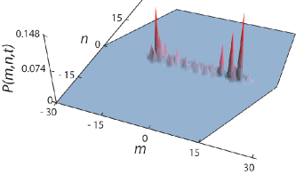
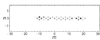
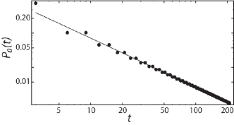
Figure 4: (Color online) Probability distribution of the walk driven by ${\cal C}_{Rec}$ and the time dependence of the probability at the origin for the initial state $\frac{1}{\sqrt{3}}(1,1,1)^{T}$. In the upper plot, we show the probability distribution after 30 steps. The center plot shows the quasi $1$-dimensional behavior of the same probability distribution on a density plot with graylevel on the log scale. The lower plot shows the $t^{-1}$ power law scaling of the probability at the origin on a loglog scale. The straight line corresponds to $t^{-1}$.

Illustrating the results above we constructed a coin operator which belongs to the class ${\cal C}^{\prime}$

$${\cal C}_{Rec}=\frac{1}{\sqrt{2}}\left(\begin{array}[]{rrr}0&0&\sqrt{2}\\ 1&1&0\\ 1&-1&0\end{array}\right)\,.$$ (38)

Let us analyze the behavior of a walk driven by ${\cal C}_{Rec}$ observing the eigenenergies given by the characteristic polynomial

$$\Theta(\omega,\mathbf{k}) = \det\left(\tilde{U}(\mathbf{k})-e^{i\omega}I\right)=$$

$$= \cos\left(k_{1}-\frac{\omega}{2}\right)-\sqrt{2}\cos\left(\frac{3\omega}{2}\right)=0\,.$$

The characteristic polynomial is independent of $k_{2}$, thus the eigenenergies are independent of $k_{2}$, too. Hence the walk is quasi $1$-dimensional (See Figure 4). Moreover, the double integral in equation (18) simplifies to a single integral, leading us back to the standard one-dimensional quantum walk stefanak_prl_2008 . The decay rate of the probability at the origin is $t^{-1}$ and the walk is recurrent, as seen in Figure 4.

V Summary

The analysis of three-state quantum walks on a triangular lattice clearly demonstrates that neither the dimension of the underlying lattice nor the dimension of the coin space in itself can determine whether localization or recurrence can occur. Although we could construct an example where the walk was recurrent, we have also proven that only the coins from the special subclass leading to quasi-onedimensional propagation allow for recurrence. We have calculated the time exponents of the probability decay at the origin for the Grover walk resulting in transience. This behavior is in sharp contrast with the recurrence properties of the Grover walk on a regular square lattices which traps the walker at the origin with finite probability, also known as localization.

The triangular lattice is one of the few solvable models allowing to decide about the recurrence properties of the quantum walk. It is certainly interesting to analyze other higher dimensional quantum walks from this perspective. The presented work is just the fist step in classifying quantum walks using the concept of recurrence and a number of interesting effects can be expected for related models.

Appendix A The classical 3-way walk on $2$-dimensional Cartesian lattice

The classical 3-way walk is strongly connected to the generalized Pascal’s triangle, the so called Pascal’s pyramid harris , in a similar way as the regular $1$-dimensional classical random walk on a line connects to Pascal’s triangle. The central element in the $t$th Pascal’s pyramid is given by

$$C_{0}(t)\equiv\frac{t!}{(t/3)!^{3}}\,.$$ (40)

This expression is only valid when $t$ is dividable by 3 (as the walker could possible return to the origin at every 3rd step). We normalize the central element, to get the probability of the walker returning

$$p_{0}(t)\equiv\frac{1}{3^{t}}C_{0}(t)=\frac{1}{3^{t}}\frac{t!}{(t/3)!^{3}}\,.$$ (41)

We approximate the return probability $p_{0}(t)$ with Stirling’s approximation

$$p_{0}(t)=\frac{1}{3^{t}}\frac{t!}{(t/3)!^{3}}\approx\frac{3\sqrt{3}}{2\pi t}\,.$$ (42)

The recurrence properties of the classical random walks are represented by the classical Pólya number revesz

$$\mathcal{P}=1-\frac{1}{S}\,,$$ (43)

where

$$S=\sum_{t=0}^{\infty}p_{0}(t)\,.$$ (44)

In our case $p_{0}(t)$ is proportional to $t^{-1}$, hence the series $S$ diverges, the classical Pólya number ($\mathcal{P}$) equals $1$, therefore the classical 3-way random walk is recurrent.

References

- (1) H. Kesten, Not. AMS 53, 572 (2006); G. Grimmett, Percolation, Springer, Berlin, Heidelberg (1999).
- (2) G. Ódor, Rev. Mod. Phys. 76, 663 (2004).
- (3) Y. V. Nazarov, Y. M. Blanter, Quantum Transport: Introduction to Nanoscience, Cambridge University Press, (2009).
- (4) P. Révész, Random walk in random and non-random environments, World Scientific, Singapore (1990).
- (5) G. Pólya, Math. Ann. 84, 149 (1921).
- (6) Y. Aharonov, L. Davidovich, and N. Zagury, Phys. Rev. A 48, 1687 (1993).
- (7) D. A. Meyer J. Stat. Phys. 85 551-574 (1996).
- (8) M. Santha, 5th Theory and Applications of Models of Computation (TAMC08), Xian, April 2008, LNCS 4978, 31-46, arXiv:quant-ph/0808.0059v1.
- (9) V. Kendon, Phil. Trans. R. Soc. A 364, 3407-3422 (2006).
- (10) J. T. Chalker and P. D. Coddington, J. Phys. C: Solid State Phys. 21 2665-2679 (1988); S. N. Dorogovtsev Phys. Solid State 40 35 (1998).
- (11) F. Zähringer, G. Kirchmair, R. Gerritsma, E. Solano, R. Blatt and C. F. Roos, Phys. Rev. Lett. 104, 100503 (2010).
- (12) M. Karski, L. Förster, J.-M. Choi, A. Steffen, W. Alt, D. Meschede and A. Widera, Science 325, 174 (2009).
- (13) A. Schreiber, K. N. Cassemiro, V. Potoček, A. Gábris, P. J. Mosley, E. Andersson, I. Jex and Ch. Silberhorn, Phys. Rev. Lett. 104, 050502 (2010).
- (14) J. Kempe Probability Theory and Related Fields, 133 215 (2005); H. Krovi and T. A. Brun, Phys. Rev. A 74, 042334 (2006); A. Kempf and R. Portugal Phys. Rev. A 79, 052317 (2009).
- (15) M. Štefaňák, I. Jex and T. Kiss, Phys. Rev. Lett. 100, 020501 (2008).
- (16) T. Kiss, L. Kecskés, M. Štefaňák and I. Jex, Phys. Scr. T135 014055 (2009).
- (17) M. Štefaňák, T. Kiss and I. Jex, Phys. Rev. A. 78, 032306 (2008).
- (18) T. D. Mackay, S. D. Bartlett, L. T. Stephenson and B. C. Sanders, J. Phys. A: Math. Gen. 35, 2745 (2002); N. Inui, Y. Konishi and N. Konno, Phys. Rev. A 69, 052323 (2004).
- (19) M. Štefaňák, T. Kiss and I. Jex, New J. Phys. 11, 043027 (2009).
- (20) N. Inui, N. Konno and E. Segawa, Phys. Rev. E, 72, 056112 (2005).
- (21) N. Inui and N. Konno, Physica A 353, 133-144 (2003).
- (22) G. Abal, R. Donangelo, F. L. Marquezino and R. Portugal, arXiv:quant-ph/1001.1139.
- (23) T. Kitagawa, M. S. Rudner, E. Berg and E. Demlerl, arXiv:cond-mat/1003.1729v1.
- (24) M. A. Jafarizadeha and R. Sufiani Physica A 381 116 (2007).
- (25) J. M. Harris, J. L. Hirst and M. J. Mossinghoff, Combinatorics and Graph Theory, Springer (2008).