Krylov-Type Methods for Tensor Computations

Abstract

Several Krylov-type procedures are introduced that generalize matrix Krylov methods for tensor computations. They are denoted minimal Krylov recursion, maximal Krylov recursion, contracted tensor product Krylov recursion. It is proved that the for a given tensor with low rank, the minimal Krylov recursion extracts the correct subspaces associated to the tensor within certain number of iterations. An optimized minimal Krylov procedure is described that gives a better tensor approximation for a given multilinear rank than the standard minimal recursion. The maximal Krylov recursion naturally admits a Krylov factorization of the tensor. The tensor Krylov methods are intended for the computation of low-rank approximations of large and sparse tensors, but they are also useful for certain dense and structured tensors for computing their higher order singular value decompositions or obtaining starting points for the best low-rank computations of tensors. A set of numerical experiments, using real life and synthetic data sets, illustrate some of the properties of the tensor Krylov methods.

1 Introduction

Large-scale problems in engineering and science often require solution of sparse linear algebra problems, such as systems of equations, and eigenvalue problems. Recently [1, 2, 6, 19, 18, 20] it has been shown that several applications in information sciences, such as web link analysis, social networks, and cross-language information retrieval, generate large data sets that are sparse tensors. In this paper we introduce new methods for efficient computations with large and sparse tensors.

Since the 1950’s Krylov subspace methods have been developed so that they are now one of the main classes of algorithms for solving iteratively large and sparse matrix problems. Given a square matrix $A\in\mathbb{R}^{n\times n}$ and a starting vector $u\in\mathbb{R}^{n}$ the corresponding $k$-dimensional Krylov subspace is

$$\mathcal{K}_{k}(A,u)=\operatorname{span}\{u,Au,A^{2}u,\dots,A^{k-1}u\}.$$

In floating point arithmetic the vectors in the Krylov subspace are useless unless they are orthonormalized. Applying Gram-Schmidt orthogonalization one obtains the Arnoldi process, which generates an orthonormal basis for the Krylov subspace $\mathcal{K}_{k}(A,u)$. In addition, the Arnoldi process generates the factorization

$$AU_{k}=U_{k+1}H_{k},$$ (1)

where $U_{k}=[u_{1}\,\dots\,u_{k}]$, and $U_{k+1}=[U_{k}\,\,u_{k+1}]$ with orthonormal columns, and $H_{k}$ is a Hessenberg matrix with the orthonormalization coefficients. Based on the factorization (1) one can compute an approximation of the solution of a linear system or an eigenvalue problem by projecting onto the space spanned by the columns of $U_{k}$, where $k$ is much smaller than the dimension of $A$; on that subspace the operator $A$ is represented by the small matrix $H_{k}$. This approach is particularly useful for large, and sparse problems, since it uses the matrix $A$ in matrix-vector multiplications only.

Projection to a low-dimensional subspace is a common technique in many areas of information science. This is also the case in applications involving tensors. One of the main theoretical and algorithmic problems researchers have addressed is the computation of low rank approximation of a given tensor [9, 26, 14, 23, 16]. The two main approaches are the Canonical Decomposition [5, 12] and the Tucker decomposition [30]; we are concerned with the latter.

The following question arises naturally:

Can Krylov methods be generalized to tensors, to be used for the projection to low-dimensional subspaces?

We answer this question in the affirmative, and describe several alternative ways one can generalize Krylov subspace methods for tensors. Our method is inspired by Golub-Kahan bidiagonalization [10], and the Arnoldi method, see e.g. [27, p. 303]. In the bidiagonalization method two sequences of orthogonal vectors are generated; for a tensor of order three, our procedures generates three sequences of orthogonal vectors. Unlike the bidiagonalization procedure, it is necessary to perform Arnoldi style orthogonalization of the generated vectors explicitly. For matrices, once an initial vector has been selected, the whole sequence is determined uniquely. For tensors, there are many ways in which the vectors can be generated. We will describe three principally different tensor Krylov methods. These are the minimal Krylov recursion, maximal Krylov recursion and contracted tensor product Krylov recursion. In addition we will discuss the implementation of an optimized version [11] of the minimal Krylov recursion, and we will show how to deal with tensors that are small in one mode. For a given tensor $\mathcal{A}$ with $\operatorname{rank}(\mathcal{A})=(p,q,r)$ the minimal Krylov recursion can extract the correct subspaces associated to $\mathcal{A}$ in $\max\{p,q,r\}$ iterations. The maximal Krylov recursion admits a tensor Krylov factorization that generalizes the matrix Krylov factorization. The contracted tensor product Krylov recursion is a generalization of the matrix Lanczos method applied to symmetric matrices $A^{\sf T}A$ and $AA^{\sf T}$.

Although our main motivation is to develop efficient methods for large and sparse tensors, the methods are useful for other tasks as well. In particular, they can be used for obtaining starting points for the best low rank tensor approximation problem, and for tensors with relatively low multilinear rank they provide a way of speeding up the computation of the Higher Order SVD (HOSVD) [7]. The latter part is done by first computing a full factorization using the minimal Krylov procedure and then computing the HOSVD of the much smaller core tensor that results from the approximation.

The paper is organized as follows. The necessary tensor concepts are introduced in Section 2. The Arnoldi and Golub-Kahan procedures are sketched in Section 3. In Section 4 we describe different variants of Krylov methods for tensors. Section 5 contains numerical examples illustrating various aspects of the proposed methods.

As this paper is a first introduction to Krylov methods for tensors, we do not imply that it gives a comprehensive treatment of the subject. Rather our aim is to outline our discoveries so far, and point to the similarities and differences between the tensor and matrix cases.

2 Tensor Concepts

2.1 Notation and Preliminaries

Tensors will be denoted by calligraphic letters, e.g $\mathcal{A},\mathcal{B}$, matrices by capital roman letters and vectors by lower case roman letters. In order not to burden the presentation with too much detail, we sometimes will not explicitly mention the dimensions of matrices and tensors, and assume that they are such that the operations are well-defined. The whole presentation will be in terms of tensors of order three, or equivalently 3-tensors. The generalization to order-$N$ tensors is obvious.

We will use the term tensor in a restricted sense, i.e. as a 3-dimensional array of real numbers, $\mathcal{A}\in\mathbb{R}^{l\times m\times n}$, where the vector space is equipped with some algebraic structures to be defined. The different “dimensions” of the tensor are referred to as modes. We will use both standard subscripts and “MATLAB-like” notation: a particular tensor element will be denoted in two equivalent ways,

$$\mathcal{A}(i,j,k)=a_{ijk}.$$

A subtensor obtained by fixing one of the indices is called a slice, e.g.,

$$\mathcal{A}(i,:,:).$$

Such a slice can be considered as an order-3 tensor, but also as a matrix.

A fibre is a subtensor, where all indices but one are fixed,

$$\mathcal{A}(i,:,k).$$

For a given third order tensor, there are three associated subspaces, one for each mode. These subspaces are given by

$$\operatorname{Range}\{\mathcal{A}(:,j,k)\;|\;j=1:m,\;k=1:n\},$$

$$\operatorname{Range}\{\mathcal{A}(i,:,k)\;|\;i=1:l,\;k=1:n\},$$

$$\operatorname{Range}\{\mathcal{A}(i,j,:)\;|\;i=1:l,\;j=1:m\}.$$

The multilinear rank [13, 8] of the tensor is said to be equal to $(p,q,r)$ if the dimension of these subspaces are $p,$ $q,$ and $r$, respectively.

It is customary in numerical linear algebra to write out column vectors with the elements arranged vertically, and row vectors with the elements horizontally. This becomes inconvenient when we are dealing with more than two modes. Therefore we will not make a notational distinction between mode-1, mode-2, and mode-3 vectors, and we will allow ourselves to write all vectors organized vertically. It will be clear from the context to which mode the vectors belong. However, when dealing with matrices, we will often talk of them as consisting of column vectors.

2.2 Tensor-Matrix Multiplication

We define multilinear multiplication of a tensor by a matrix as follows. For concreteness we first present multiplication by one matrix along the first mode and later for all three modes simultaneously. The mode-$1$ product of a tensor $\mathcal{A}\in\mathbb{R}^{l\times m\times n}$ by a matrix $U\in\mathbb{R}^{p\times l}$ is defined

$$\mathbb{R}^{p\times m\times n}\ni\mathcal{B}=\bm{\left(}U\bm{}_{1}\bm{\cdot}\mathcal{A},\qquad b_{ijk}=\sum_{\alpha=1}^{l}u_{i\alpha}a_{\alpha jk}.$$ (2)

This means that all mode-$1$ fibres in the $3$-tensor $\mathcal{A}$ are multiplied by the matrix $U$. Similarly, mode-$2$ multiplication by a matrix $V\in\mathbb{R}^{q\times m}$ means that all mode-$2$ fibres are multiplied by the matrix $V$. Mode-$3$ multiplication is analogous. With a third matrix $W\in\mathbb{R}^{r\times n}$, the tensor-matrix multiplication in all modes is given by

$$\mathbb{R}^{p\times q\times r}\ni\mathcal{B}=\bm{\left(}U,V,W\bm{}\bm{\cdot}\mathcal{A},\qquad b_{ijk}=\sum_{\alpha,\beta,\gamma=1}^{l,m,n}u_{i\alpha}v_{j\beta}w_{k\gamma}a_{\alpha\beta\gamma},$$ (3)

where the mode of each multiplication is understood from the order in which the matrices are given.

It is convenient to introduce a separate notation for multiplication by a transposed matrix $\bar{U}\in\mathbb{R}^{l\times p}$:

$$\mathbb{R}^{p\times m\times n}\ni\mathcal{C}=\bm{\left(}\bar{U}^{\sf T}\bm{}_{1}\bm{\cdot}\mathcal{A}=\mathcal{A}\bm{\cdot}\bm{\left(}\bar{U}\bm{}_{1},\qquad c_{ijk}=\sum_{\alpha=1}^{l}a_{\alpha jk}\bar{u}_{\alpha i}.$$ (4)

Let $u\in\mathbb{R}^{l}$ be a vector and $\mathcal{A}\in\mathbb{R}^{l\times m\times n}$ a tensor. Then

$$\mathbb{R}^{1\times m\times n}\ni\mathcal{B}:=\bm{\left(}u^{\sf T}\bm{}_{1}\bm{\cdot}\mathcal{A}=\mathcal{A}\bm{\cdot}\bm{\left(}u\bm{}_{1}\equiv B\in\mathbb{R}^{m\times n}.$$ (5)

Thus we identify a tensor with a singleton dimension with a matrix. Similarly, with $u\in\mathbb{R}^{l}$ and $w\in\mathbb{R}^{n}$, we will identify

$$\mathbb{R}^{1\times m\times 1}\ni\mathcal{C}:=\mathcal{A}\bm{\cdot}\bm{\left(}u,w\bm{}_{1,3}\equiv c\in\mathbb{R}^{m},$$ (6)

i.e., a tensor of order three with two singleton dimensions is identified with a vector, here in the second mode. Since formulas like (6) have key importance in this paper, we will state the other two versions as well;

$$\mathcal{A}\bm{\cdot}\bm{\left(}u,v\bm{}_{1,2}\in\mathbb{R}^{n},\qquad\mathcal{A}\bm{\cdot}\bm{\left(}v,w\bm{}_{2,3}\in\mathbb{R}^{l},$$ (7)

where $v\in\mathbb{R}^{m}$.

2.3 Inner Product, Norm, and Contractions

Given two tensors $\mathcal{A}$ and $\mathcal{B}$ of the same dimensions, we define the inner product,

$$\langle\mathcal{A},\mathcal{B}\rangle=\sum_{\alpha,\beta,\gamma}a_{\alpha\beta\gamma}b_{\alpha\beta\gamma}.$$ (8)

The corresponding tensor norm is

$$\|\mathcal{A}\|=\langle\mathcal{A},\mathcal{A}\rangle^{1/2}.$$ (9)

This Frobenius norm will be used throughout the paper. As in the matrix case, the norm is invariant under orthogonal transformations, i.e.

$$\|\mathcal{A}\|=\left\|\bm{\left(}U,V,W\bm{}\bm{\cdot}\mathcal{A}\right\|=\|\mathcal{A}\bm{\cdot}\bm{\left(}P,Q,S\bm{}\|,$$

for orthogonal matrices $U$, $V$, $W$, $P$, $Q$, and $S$. This is obvious from the fact that multilinear multiplication by orthogonal matrices does not change the Euclidean length of the corresponding fibres of the tensor.

For convenience we will denote the inner product of vectors $x$ and $y$ in any mode (but, of course, the same) by $x^{\sf T}y$. Let $v=\mathcal{A}\bm{\cdot}\bm{\left(}u,w\bm{}_{1,3}$; then, for a matrix $V=[v_{1}\;v_{2}\;\cdots\;v_{p}]$ of mode-2 vectors, we have

$$V^{\sf T}v=\bm{\left(}V^{\sf T}\bm{}_{2}\bm{\cdot}(\mathcal{A}\bm{\cdot}\bm{\left(}u,w\bm{}_{1,3})=\mathcal{A}\bm{\cdot}\bm{\left(}u,V,w\bm{}\in\mathbb{R}^{1\times p\times 1}.$$

The following well-known result will be needed.

Lemma 1.

Let $\mathcal{A}\in\mathbb{R}^{l\times m\times n}$ be given along with three matrices with orthonormal columns, $U\in\mathbb{R}^{l\times p}$, $V\in\mathbb{R}^{m\times q}$, and $W\in\mathbb{R}^{n\times r}$, where $p\leq l$, $q\leq m$, and $r\leq n$. Then the least squares problem

$$\min_{\mathcal{S}}\|\mathcal{A}-\bm{\left(}U,V,W\bm{}\bm{\cdot}\mathcal{S}\|$$

has the unique solution

$$\mathcal{S}=\bm{\left(}U^{\sf T},V^{\sf T},W^{\sf T}\bm{}\bm{\cdot}\mathcal{A}=\mathcal{A}\bm{\cdot}\bm{\left(}U,V,W\bm{}.$$

The elements of the tensor $\mathcal{S}$ are given by

$$s_{\lambda\mu\nu}=\mathcal{A}\bm{\cdot}\bm{\left(}u_{\lambda},v_{\mu},w_{\nu}\bm{},\quad 1\leq\lambda\leq p,\quad 1\leq\mu\leq q,\quad 1\leq\nu\leq r.$$ (10)

Proof.

The proof is a straightforward generalization of the corresponding proof for matrices. Enlarge each of the matrices so that it becomes square and orthogonal, i.e., put

$$\bar{U}=[U\,\,U_{\perp}],\quad\bar{V}=[V\,\,V_{\perp}],\quad\bar{W}=[W\,\,W_{\perp}].$$

Introducing the residual $\mathcal{R}=\mathcal{A}-\bm{\left(}U,V,W\bm{}\bm{\cdot}\mathcal{S}$ and using the invariance of the norm under orthogonal transformations, we get

$$\|\mathcal{R}\|^{2}=\left\|\mathcal{R}\bm{\cdot}\bm{\left(}\bar{U},\bar{V},\bar{W}\bm{}\right\|^{2}=\|\mathcal{A}\bm{\cdot}\bm{\left(}U,V,W\bm{}-\mathcal{S}\|^{2}+C^{2},$$

where $C^{2}=\|\mathcal{A}\bm{\cdot}\bm{\left(}U_{\perp},V_{\perp},W_{\perp}\bm{}\|^{2}$ does not depend on $\mathcal{S}$. The relation (10) is obvious from the definition of tensor-matrix product. ∎

The inner product (8) can be considered as a special case of the contracted product of two tensors, cf. [17, Chapter 2], which is a tensor (outer) product followed by a contraction along specified modes. Thus, if $\mathcal{A}$ and $\mathcal{B}$ are $3$-tensors, we define, using essentially the notation of [3],

$$\mathcal{C} =\left\langle\mathcal{A},\mathcal{B}\right\rangle_{1}\,, c_{jkj^{\prime}k^{\prime}} =\sum_{\alpha}a_{\alpha jk}b_{\alpha j^{\prime}k^{\prime}}\,, \mbox{($4$-tensor)}\,,$$ (11.a)

$$D =\left\langle\mathcal{A},\mathcal{B}\right\rangle_{1,2}\,, d_{kk^{\prime}} =\sum_{\alpha,\beta}a_{\alpha\beta k}b_{\alpha\beta k^{\prime}}\,, \mbox{($2$-tensor)},$$ (11.b)

$$e =\langle\mathcal{A},\mathcal{B}\rangle=\left\langle\mathcal{A},\mathcal{B}\right\rangle_{1\dots 3}\,, e =\sum_{\alpha,\beta,\gamma}a_{\alpha\beta\gamma}b_{\alpha\beta\gamma}\,, \mbox{(scalar)}.$$ (11.c)

It is required that the contracted dimensions are equal in the two tensors. We will refer to the first two as partial contractions. The subscript 1 in $\langle\mathcal{A},\mathcal{B}\rangle_{1}$ and 1,2 in $\langle\mathcal{A},\mathcal{B}\rangle_{1,2}$ indicate that the contraction is over the first mode in both arguments and in the first and second mode in both arguments, respectively. It is also convenient to introduce a notation when contraction is performed in all but one mode. For example the product in (11.b) may also be written

$$\left\langle\mathcal{A},\mathcal{B}\right\rangle_{1,2}\equiv\left\langle\mathcal{A},\mathcal{B}\right\rangle_{-3}\,.$$ (12)

The definition of contracted products is valid also when the tensors are of different order. The only assumption is that the dimension of the correspondingly contracted modes are the same in the two arguments. The dimensions of the resulting product are in the order given by the non-contracted modes of the first argument followed by the non-contracted modes of the second argument.

2.4 Tensor Matricization

Later on we will also need the notion of tensor matricization. Any given third order tensor $\mathcal{A}\in\mathbb{R}^{l\times m\times n}$ can be matricized alone its different modes. These matricizations will be written as $A^{(1)}$, which is an $l\times mn$ matrix, $A^{(2)}$, which is an $m\times ln$ matrix, and $A^{(3)}$ is an $n\times lm$ matrix. The exact relations of the entries of $\mathcal{A}$ to the three different matricizations can be found in [9]. It is sufficient, for our needs in this paper, to recall that the matricizations of a given multilinear tensor-matrix product $\mathcal{B}=\bm{\left(}U,V,W\bm{}\bm{\cdot}\mathcal{A}$ have the following forms:

$$B^{(1)} =UA^{(1)}(V\otimes W)^{\sf T},$$

$$B^{(2)} =VA^{(2)}(U\otimes W)^{\sf T},$$

$$B^{(3)} =WA^{(3)}(U\otimes V)^{\sf T}.$$

3 Two Krylov Methods for Matrices

In this section we will describe briefly the two matrix Krylov methods that are the starting point of our generalization to tensor Krylov methods.

3.1 The Arnoldi Procedure

The Arnoldi procedure is used to compute a low-rank approximation/factorization (1) of a square, in general nonsymmetric matrix $A$. It requires a starting vector $u_{1}=:U_{1}$ (or, alternatively, $v_{1}=:V_{1}$), and in each step the new vector is orthogonalized against all previous vectors using the modified Gram-Schmidt process. We present the Arnoldi procedure in the style of [27, p. 303].

Algorithm 1 Arnoldi Procedure

  for $i=1,2,\ldots,k$ do

     1 $h_{i}=U_{i}^{\sf T}Au_{i}$

     2 $h_{i+1,i}u_{i+1}=Au_{i}-U_{i}h_{i}$

     3 $U_{i+1}=[U_{i}\;u_{i+1}]$

     4 $H_{i}=\begin{bmatrix}H_{i-1}&h_{i}\\ 0&h_{i+1,i}\end{bmatrix}$

  end for

The constant $h_{i+1,i}$ is used to normalize the new vector to length one. Note that the matrix $H_{k}$ in the the factorization (1) is obtained by collecting the orthonormalization coefficients $h_{i}$ and $h_{i+1,i}$ in an upper Hessenberg matrix.

3.2 Golub-Kahan Bidiagonalization

Let $A\in\mathbb{R}^{m\times n}$ be a matrix, and let $\beta_{1}u_{1},v_{0}=0$, where $\|u_{1}\|=1$, be starting vectors. The Golub-Kahan bidiagonalization procedure [10] is defined by the following recursion.

Algorithm 2 Golub-Kahan bidiagonalization

  for $i=1,2,\dots,k$ do

     1 $\alpha_{i}v_{i}=A^{\sf T}u_{i}-\beta_{i}v_{i-1}$

     2 $\beta_{i+1}u_{i+1}=Av_{i}-\alpha_{i}u_{i}$

  end for

The scalars $\alpha_{i},\,\beta_{i}$ are chosen to normalize the generated vectors $v_{i},u_{i}$. Forming the matrices $U_{k+1}=[u_{1}\,\cdots\,u_{k+1}]\in\mathbb{R}^{m\times(k+1)}$ and $V_{k}=[v_{1}\,\cdots\,v_{k}]\in\mathbb{R}^{n\times k}$, it is straightforward to show that

$$AV_{k}=U_{k+1}B_{k+1},\qquad A^{\sf T}U_{k}=V_{k}\widehat{B}_{k},$$ (13)

where $V_{k}^{\sf T}V_{k}=I,\;U_{k+1}^{\sf T}U_{k+1}=I,$ and

$$B_{k+1}=\begin{bmatrix}\alpha_{1}&&&\\ \beta_{2}&\alpha_{2}&&\\ &\ddots&\ddots&\\ &&\beta_{k}&\alpha_{k}\\ &&&\beta_{k+1}\\ \end{bmatrix}=\begin{bmatrix}\widehat{B}_{k}\\ \beta_{k+1}e_{k}^{\sf T}\end{bmatrix}\in\mathbb{R}^{(k+1)\times k}$$ (14)

is bidiagonal.

Using tensor notation from Section 2.2, and a special case of the identification (6), we may express the two steps of the recursion as

Algorithm 3 Golub-Kahan bidiagonalization in tensor notation

  for $i=1,2,\dots,k$ do

     1 $\alpha_{i}v_{i}=A\bm{\cdot}\bm{\left(}u_{i}\bm{}_{1}-\beta_{i}v_{i-1}$

     2 $\beta_{i+1}u_{i+1}=A\bm{\cdot}\bm{\left(}v_{i}\bm{}_{2}-\alpha_{i}u_{i}$

  end for

We observe that the $u_{i}$ vectors “live” in the first mode of $A$, and we generate the sequence $u_{2},u_{3},\ldots$, by multiplication of the $v_{i}$ vectors in the second mode, and vice versa.

4 Tensor Krylov Methods

4.1 A Minimal Krylov Recursion

In this subsection we will present the main process for the tensor Krylov methods. We will further prove that, for tensors with $\operatorname{rank}(\mathcal{A})=(p,q,r)$, we can capture all three subspaces associated to $\mathcal{A}$ within $\max\{p,q,r\}$ steps of the algorithms. Finally we will state a partial factorization that is induced by the procedure.

Let $\mathcal{A}\in\mathbb{R}^{l\times m\times n}$ be a given tensor of order three. It is now straightforward to generalize the Golub-Kahan procedure, starting from Algorithm 3. Assuming we have two starting vectors, $u_{1}\in\mathbb{R}^{l}$ and $v_{1}\in\mathbb{R}^{m}$ we can obtain a third mode vector $w_{1}=\mathcal{A}\bm{\cdot}\bm{\left(}u_{1},v_{1}\bm{}_{1,2}\in\mathbb{R}^{n}$. We can then generate three sequences of vectors

$$u_{i+1} =\mathcal{A}\bm{\cdot}\bm{\left(}v_{i},w_{i}\bm{}_{2,3},$$ (15)

$$v_{i+1} =\mathcal{A}\bm{\cdot}\bm{\left(}u_{i},w_{i}\bm{}_{1,3},$$ (16)

$$w_{i+1} =\mathcal{A}\bm{\cdot}\bm{\left(}u_{i},v_{i}\bm{}_{1,2},$$ (17)

for $i=1,\dots,k$. We see that the first mode sequence of vectors $(u_{i+1})$ are generated by multiplication of second and third mode vectors $(v_{i})$ and $(w_{i})$ by the tensor $\mathcal{A}$, and similarly for the other two sequences. The newly generated vector is immediately orthogonalized against all the previous ones in its mode, using the modified Gram-Schmidt process. An obvious alternative to (16) and (17) that is consistent with the Golub-Kahan recursion is to use the most recent vectors in computing the new one. This recursion is presented in Algorithm 4. In the algorithm description it is understood that $U_{i}=[u_{1}\,u_{2}\,\cdots\,u_{i}]$, etc. The coefficients  $\alpha_{u}$, $\alpha_{v}$, and $\alpha_{w}$ are used to normalize the generated vectors to length one.

For reasons that will become clear later, we will refer to this recursion as a minimal Krylov recursion.

Algorithm 4 Minimal Krylov recursion

  Given: two normalized starting vectors $u_{1}$ and $v_{1}$,

  $\alpha_{w}w_{1}=\mathcal{A}\bm{\cdot}\bm{\left(}u_{1},v_{1}\bm{}_{1,2}$

  for $i=1,2,\ldots,k-1$ do

     $\widehat{u}=\mathcal{A}\bm{\cdot}\bm{\left(}v_{i},w_{i}\bm{}_{2,3};\quad h_{u}=U_{i}^{\sf T}\widehat{u}$

     $\alpha_{u}u_{i+1}=\widehat{u}-U_{i}h_{u}$;  $H_{i}^{u}=\begin{bmatrix}H_{i}^{u}&h_{u}\\ 0&\alpha_{u}\end{bmatrix}$

     $\widehat{v}=\mathcal{A}\bm{\cdot}\bm{\left(}u_{i+1},w_{i}\bm{}_{1,3};\quad h_{v}=V_{i}^{\sf T}\widehat{v}$

     $\alpha_{v}v_{i+1}=\widehat{v}-V_{i}h_{v}$;  $H_{i}^{v}=\begin{bmatrix}H_{i}^{u}&h_{v}\\ 0&\alpha_{v}\end{bmatrix}$

     $\widehat{w}=\mathcal{A}\bm{\cdot}\bm{\left(}u_{i+1},v_{i+1}\bm{}_{1,2};\quad h_{w}=W_{i}^{\sf T}\widehat{w}$

     $\alpha_{w}w_{i+1}=\widehat{w}-W_{i}h_{w}$;  $H_{i}^{w}=\begin{bmatrix}H_{i}^{w}&h_{w}\\ 0&\alpha_{w}\end{bmatrix}$

  end for

The process may break down, i.e. we obtain a new vector $u_{i+1}$, for instance, which is linear combination of the vectors in $U_{i}$. This can happen in two principally different situations. The first one is when, for example, the vectors in $U_{i}$ span the range space of $A^{(1)}$. If this is the case we are done generating new $u$-vectors. The second case is when we get a “true breakdown”, $u_{i+1}$ is a linear combination of vectors in $U_{i}$, but $U_{i}$ does not span the entire range space of $A^{(1)}$. This can be fixed by taking a vector $u_{i+1}\perp U_{i}$ with $u_{i+1}$ in range of $A^{(1)}$.

4.1.1 Tensors with Given Cubical Ranks

Assume that the $l\times m\times n$ tensor has a cubical low rank, i.e. $\operatorname{rank}(\mathcal{A})=(r,r,r)$ with $r\leq\min\{l,m,n\}$. Then there exist a tensor $\mathcal{C}\in\mathbb{R}^{r\times r\times r}$, and full column rank matrices $X,Y,Z$ such that $\mathcal{A}=\bm{\left(}X,Y,Z\bm{}\bm{\cdot}\mathcal{C}$.

We will now prove that, when the starting vectors $u_{1}$, $v_{1}$ and $w_{1}$ are in the range of the respective subspaces, the minimal Krylov procedure generates matrices $U,V,W$, such that $\operatorname{span}(U)=\operatorname{span}(X)$, $\operatorname{span}(V)=\operatorname{span}(Y)$ and $\operatorname{span}(W)=\operatorname{span}(Z)$ after $r$ steps. Of course, for the low multilinear rank approximation problem of tensors it is the subspaces that are important, not their actual representation. The specific basis spanning e.g. $\operatorname{span}(X)$ is ambiguous.

Theorem 2.

Let $\mathcal{A}=\bm{\left(}X,Y,Z\bm{}\bm{\cdot}\mathcal{C}\in\mathbb{R}^{l\times m\times n}$ with $\operatorname{rank}(\mathcal{A})=(r,r,r)$. Assume we have starting vectors in the associated range spaces, i.e. $u_{1}\in\operatorname{span}(X)$, $v_{1}\in\operatorname{span}(Y)$, $w_{1}\in\operatorname{span}(Z)$. Assume also that the process does not break down within $r$ iterations. Then the minimal Krylov procedure in Algorithm 4 generates matrices $U_{r},V_{r},W_{r}$ with

$$\operatorname{span}(U_{r})=\operatorname{span}(X),\quad\operatorname{span}(V_{r})=\operatorname{span}(Y),\quad\operatorname{span}(W_{r})=\operatorname{span}(Z).$$

Proof.

First observe that the recursion generates vectors in the span of $X$, $Y$, and $Z$, respectively:

$$\mathcal{A}\bm{\cdot}\bm{\left(}v,w\bm{}_{2,3} =\mathcal{C}\bm{\cdot}\bm{\left(}X^{\sf T},Y^{\sf T}v,Z^{\sf T}w\bm{}=\mathcal{C}\bm{\cdot}\bm{\left(}X^{\sf T},\bar{v},\bar{w}\bm{}=Xc_{1},$$

$$\mathcal{A}\bm{\cdot}\bm{\left(}u,w\bm{}_{1,3} =\mathcal{C}\bm{\cdot}\bm{\left(}X^{\sf T}u,Y^{\sf T},Z^{\sf T}w\bm{}=\mathcal{C}\bm{\cdot}\bm{\left(}\bar{u},Y^{\sf T},\bar{w}\bm{}=Yc_{2},$$

$$\mathcal{A}\bm{\cdot}\bm{\left(}u,v\bm{}_{1,2} =\mathcal{C}\bm{\cdot}\bm{\left(}X^{\sf T}u,Y^{\sf T}v,Z^{\sf T}\bm{}=\mathcal{C}\bm{\cdot}\bm{\left(}\bar{u},\bar{v},Z^{\sf T}\bm{}=Zc_{3},$$

where in the first equation $\bar{v}=Y^{\sf T}v$, $\bar{w}=Z^{\sf T}w$ and $c_{1}=\mathcal{C}\bm{\cdot}\bm{\left(}\bar{v},\bar{w}\bm{}_{2,3}$, and the other two equations are analogous. Consider the first mode vector $u$. Clearly it is a linear combination of the column vectors in $X$. Since we orthonormalize every newly generated $u$-vector against all the previous vectors, and since we assume that the process does not break down, it follows that $\dim(\operatorname{span}([u_{1}\,\cdots\,u_{k}]))=k$ for $k\leq r$ will increase by one with every new $u$-vector. Given that $u_{1}\in\operatorname{span}(X)$ then for $k=r$ we have that $\operatorname{span}([u_{1}\,\cdots\,u_{r}])=\operatorname{span}(X)$. The proof is analogous for the second and third modes. ∎

We would like to make e few remarks on this theorem:

Remark (1)

It is straightforward to show that when the starting vectors are not in the associated range spaces we would only need to do one more iteration, i.e. in total $r+1$ iterations, to obtain matrices $U_{r+1}$, $V_{r+1}$ and $W_{r+1}$ that would span the column spaces of $X$, $Y$ and $Z$, respectively.

Remark (2)

It is easy to obtain starting vectors $u_{1}\in\operatorname{span}(X)$, $v_{1}\in\operatorname{span}(Y)$ and $w_{1}\in\operatorname{span}(Z)$. Choose any single nonzero mode-$k$ vector or the mean of the mode-$k$ vectors.

Remark (3)

Even if we do not choose starting vectors in the range spaces of $X,Y,Z$ and run the minimal Krylov procedure $r+1$ steps we can easily obtain a matrix $U_{r}$ spanning the correct subspaces. To do this just observe that $U_{r+1}^{\sf T}A^{(1)}=U_{r+1}^{\sf T}XC^{(1)}(Y\otimes Z)^{\sf T}$ is an $(r+1)\times mn$ matrix with rank $r$.

4.1.2 Tensors with General Low Multilinear Rank

Next we discuss the case when the tensor $\mathcal{A}\in\mathbb{R}^{l\times m\times n}$ has $\operatorname{rank}(\mathcal{A})=(p,q,r)$ with $p<l$, $q<m,$ and $r<n$. Without loss of generality we can assume $p\leq q\leq r$. Then $\mathcal{A}=\bm{\left(}X,Y,Z\bm{}\bm{\cdot}\mathcal{C}$ where $\mathcal{C}$ is a $p\times q\times r$ tensor and $X,Y,Z$ are full column rank matrices with conformal dimensions. The discussion assumes exact arithmetic and that no breakdown occurs.

From the proof of Theorem 2 we see that the vectors generated are in the span of $X$, $Y$, and $Z$, respectively. Therefore, after having performed $p$ steps we will not be able to generate any new vector in the first mode. This can be detected from the fact that the result of the orthogonalization is zero. We can now continue generating vectors in the second and third modes, using any of the first mode vectors, or a (possibly random) linear combination of them. This can be repeated until we have generated $q$ vectors in the second and third modes. The final $r-q$ mode-3 vectors can then be generated using combinations of mode-1 and mode-2 vectors that have not been used before, or, alternatively, random linear combinations of previously generated mode-1 and mode-2 vectors. We refer to the procedure described in this paragraph as the modified minimal Krylov recursion.

Theorem 3.

Let $\mathcal{A}\in\mathbb{R}^{l\times m\times n}$ be a tensor of $\operatorname{rank}(\mathcal{A})=(p,q,r)$ with $p\leq q\leq r$. We can then write $\mathcal{A}=\bm{\left(}X,Y,Z\bm{}\bm{\cdot}\mathcal{C}$, where $\mathcal{C}$ is a $p\times q\times r$ tensor and $X,Y,Z$ are full column rank matrices with conforming dimensions. Assume that the starting vectors satisfy $u_{1}\in\operatorname{span}{(X)}$, $v_{1}\in\operatorname{span}{(Y)}$ and $w_{1}\in\operatorname{span}{(Z)}$. Assume also that the process does not break down except when we obtain a set of vectors spanning the full range spaces of the different modes. Then in exact arithmetic, and in a total of $r$ steps the modified minimal Krylov recursion produces matrices $U_{p}$, $V_{q}$ and $W_{r}$, which span the same subspaces as $X,Y$, and $Z$, respectively.

The actual numerical implementation of the procedure in floating point arithmetic is, of course, much more complicated. For instance, the ranks will never be exact, so one must devise a criterion for determining the numerical ranks that will depend on the choice of tolerances. This will be the topic of our future research.

4.1.3 Partial Factorization

To our knowledge there is no simple way of writing the minimal Krylov recursion directly as a tensor Krylov factorization, analogous to (13). However, having generated three orthonormal matrices $U_{k}$, $V_{k},$ and $W_{k}$, we can easily compute a low-rank tensor approximation of $\mathcal{A}$ using Lemma 1,

$$\mathcal{A}\approx\bm{\left(}U_{k},V_{k},W_{k}\bm{}\bm{\cdot}\mathcal{H},\qquad\mathcal{H}=\bm{\left(}U_{k}^{\sf T},V_{k}^{\sf T},W_{k}^{\sf T}\bm{}\bm{\cdot}\mathcal{A}\in\mathbb{R}^{k\times k\times k}.$$ (18)

Obviously, $\mathcal{H}_{\lambda\mu\nu}=\mathcal{A}\bm{\cdot}\bm{\left(}u_{\lambda},v_{\mu},w_{\nu}\bm{}$. Comparing with Algorithm 4 we see that $\mathcal{H}$ contains elements from the Hessenberg matrices $H^{u},H^{v},H^{w}$, which contain the orthogonalization and normalization coefficients. However, not all the elements in $\mathcal{H}$ are generated in the recursion, only those that are close to the “diagonals”. Observe also that $\mathcal{H}$ has $k^{3}$ elements, whereas the minimal Krylov procedure generates three matrices with total number of $3k^{2}$ elements. We now show that the minimal Krylov procedure induces a certain partial tensor-Krylov factorization.

Proposition 4.

Assume that $U_{k}$, $V_{k}$, and $W_{k}$ have been generated by the minimal Krylov recursion and that $\mathcal{H}=\mathcal{A}\bm{\cdot}\bm{\left(}U_{k},V_{k},W_{k}\bm{}$. Then, for $1\leq i\leq k-1$,

$$(\mathcal{A}\bm{\cdot}\bm{\left(}V_{k},W_{k}\bm{}_{2,3})(:,i,i) =(\bm{\left(}U_{k}\bm{}_{1}\bm{\cdot}\mathcal{H})(:,i,i)=U_{k}H^{u}(:,i),$$ (19)

$$(\mathcal{A}\bm{\cdot}\bm{\left(}U_{k},W_{k}\bm{}_{1,3})(i+1,:,i) =(\bm{\left(}V_{k}\bm{}_{2}\bm{\cdot}\mathcal{H})(i+1,:,i)=V_{k}H^{v}(:,i),$$ (20)

$$(\mathcal{A}\bm{\cdot}\bm{\left(}U_{k},V_{k}\bm{}_{1,2})(i+1,i+1,:) =(\bm{\left(}W_{k}\bm{}_{3}\bm{\cdot}\mathcal{H})(i+1,i+1,:)=W_{k}H^{w}(:,i).$$ (21)

Proof.

Let $1\leq i\leq k-1$ and consider the fiber

$$\mathcal{H}(:,i,i)=[h_{2ii}\;\;h_{2ii}\;\;\cdots\;\;h_{i+1,ii}\;\;h_{i+2,ii}\;\;\cdots\;\;h_{kii}]^{\sf T}$$

Since, from the minimal recursion,

$$\mathcal{A}\bm{\cdot}\bm{\left(}v_{i},w_{i}\bm{}_{2,3}=\sum_{\lambda=1}^{i+1}h_{\lambda ii}u_{\lambda}=U_{i+1}H^{u}_{i}(:,i),$$

we have, for $i+2\leq s\leq k$,

$$h_{sii}=\mathcal{A}\bm{\cdot}\bm{\left(}u_{s},v_{i},w_{i}\bm{}=\bm{\left(}u_{s}^{\sf T}\bm{}_{1}\bm{\cdot}(\mathcal{A}\bm{\cdot}\bm{\left(}v_{i},w_{i}\bm{}_{2,3})=0.$$

Thus $h_{i+2,ii}=\ldots=h_{kii}=0.$ Therefore, the fiber in the left hand side of (19) is equivalent to the minimal recursion for computing $u_{i+1}$. The rest of the proof is analogous. ∎

If the sequence of vectors is generated according to Equations (15)–(17), then a similar (and simpler) proposition will hold. For example we would have

$$(\mathcal{A}\bm{\cdot}\bm{\left(}U_{k},W_{k}\bm{}_{1,3})(i,:,i)=\bm{\left(}V_{k}\bm{}_{2}\bm{\cdot}\mathcal{H}(i,:,i)=V_{k}H^{v}(:,i),\quad i=1,\dots,k.$$

4.2 A Maximal Krylov Recursion

Note that when a new $u_{i+1}$ is generated in the minimal Krylov procedure, then we use the most recently computed $v_{i}$ and $w_{i}$. In fact, we might choose any combination of previously computed $\{v_{1},v_{2},\dots,v_{i}\}$ and $\{w_{1},\dots,w_{i}\}$ that have not been used before to generate a $u$-vector. Let $\ j\leq i$ and $k\leq i$, and consider the computation of a new $u$-vector, which we may write

  $h_{u}=U_{i}^{\sf T}(\mathcal{A}\bm{\cdot}\bm{\left(}v_{j},w_{k}\bm{}_{2,3})$

  $h_{*jk}u_{i+1}=\mathcal{A}\bm{\cdot}\bm{\left(}v_{j},w_{k}\bm{}_{2,3}-U_{i}h_{u}$

Thus if we are prepared to use all previously computed $v$- and $w$-vectors, then we have a much richer combinatorial structure, which we illustrate in the following diagram. Assume that $u_{1}$ and $v_{1}$ are given. In the first steps of the maximal Krylov procedure the following vectors can be generated by combining previous vectors.

1: $$\{u_{1}\}\times\{v_{1}\}\quad \longrightarrow\quad w_{1}$$

2: $$\{v_{1}\}\times\{w_{1}\}\quad \longrightarrow\quad u_{2}$$

3: $$\{u_{1},u_{2}\}\times\{w_{1}\}\quad \longrightarrow\quad\{v_{2}\;v_{3}\}$$

4: $$\{u_{1},u_{2}\}\times\{v_{1},v_{2},v_{3}\}\quad \longrightarrow\quad\{(w_{1}),w_{2},w_{3},w_{4},w_{5},w_{6}\}$$

5: $$\{v_{1},v_{2},v_{3}\}\times\{w_{1},w_{2},\dots,w_{6}\}\quad \longrightarrow\quad\{(u_{2}),u_{3},\dots,u_{19}\}$$

6: $$\{u_{1},u_{2},\dots,u_{19}\}\times\{w_{1},w_{2},\dots,w_{6}\}\quad \longrightarrow\quad\{(v_{2}),(v_{3}),v_{4},\dots,v_{115}\}$$

Vectors computed at a previous step are within parentheses. Of course, we can only generate new orthogonal vectors as long as the total number of vectors is smaller than the dimension of that mode. Further, if at a certain stage in the procedure we have generated $\alpha$ and $\beta$ vectors in two modes, then we can generate altogether $\gamma=\alpha\beta$ vectors in the third mode (where we do not count the starting vector in that mode, if there was one).

We will now describe the first three steps in some detail. Two starting vectors $u_{1}$ and $v_{1}$, in the first and second mode, respectively. We also assume that $\|u_{1}\|=\|v_{1}\|=1$. The normalization and orthogonalization coefficients will be stored in a tensor $\mathcal{H}$. Its entries are denoted with $h_{ijk}=\mathcal{H}(i,j,k)$. Also when subscripts are written on tensor $\mathcal{H}$, they will indicate the dimensions of the tensor, e.g. $\mathcal{H}_{211}$ is a $2\times 1\times 1$ tensor.

Step (1)

In the first step we generate an new third mode vector by computing

$$\mathcal{A}\bm{\cdot}\bm{\left(}u_{1},v_{1}\bm{}_{1,2}=h_{111}w_{1}=\bm{\left(}w_{1}\bm{}_{3}\bm{\cdot}\mathcal{H}_{111},$$ (22)

where $h_{111}=\mathcal{H}_{111}$ is a normalization constant.

Step (2)

Here we compute a new first mode vector;

$$\widehat{u}_{2}=\mathcal{A}\bm{\cdot}\bm{\left(}v_{1},w_{1}\bm{}_{2,3}.$$

The orthogonalization coefficient satisfies

$$u_{1}^{\sf T}\widehat{u}_{2}=u_{1}^{\sf T}(\mathcal{A}\bm{\cdot}\bm{\left(}v_{1},w_{1}\bm{}_{2,3})=\mathcal{A}\bm{\cdot}\bm{\left(}u_{1},v_{1},w_{1}\bm{}=w_{1}^{\sf T}(\mathcal{A}\bm{\cdot}\bm{\left(}u_{1},v_{1}\bm{}_{1,2})=h_{111},$$ (23)

from (22). After orthogonalization and normalization,

$$h_{211}u_{2}=\widehat{u}_{2}-h_{111}u_{1},$$ (24)

and rearranging the terms in (24), we have the following tensor-Krylov factorization

$$\mathcal{A}\bm{\cdot}\bm{\left(}v_{1},w_{1}\bm{}_{2,3}=\bm{\left(}[u_{1},\,u_{2}]\bm{}_{1}\bm{\cdot}\mathcal{H}_{211},\qquad\mathcal{H}_{211}=\begin{bmatrix}h_{111}\\ h_{211}\end{bmatrix}.$$

Step (3)

In the third step we obtain two second mode vectors. To get $v_{2}$ we compute

$$\widehat{v}_{2}=\mathcal{A}\bm{\cdot}\bm{\left(}u_{1},w_{1}\bm{}_{1,3},\qquad h_{121}v_{2}=\widehat{v}_{2}-h_{111}v_{1};$$

the orthogonalization coefficient becomes $h_{111}$ using an argument analogous to that in (23).

Combining $u_{2}$ with $w_{1}$ will yield $v_{3}$ as follows; first we compute

$$\widehat{v}_{3}=\mathcal{A}\bm{\cdot}\bm{\left(}u_{2},w_{1}\bm{}_{1,3},$$

and orthogonalize

$$v_{1}^{\sf T}\widehat{v}_{3}=\mathcal{A}\bm{\cdot}\bm{\left(}u_{2},v_{1},w_{1}\bm{}=u_{2}^{\sf T}(\mathcal{A}\bm{\cdot}\bm{\left(}v_{1},w_{1}\bm{}_{2,3})=u_{2}^{\sf T}\widehat{u}_{2}=h_{211}.$$

We see from (24) that $h_{211}$ is already computed. The second orthogonalization becomes

$$v_{2}^{\sf T}\widehat{v}_{3}=\mathcal{A}\bm{\cdot}\bm{\left(}u_{2},v_{2},w_{1}\bm{}=:h_{221}.$$

Then

$$\qquad h_{231}v_{3}=\widehat{v}_{3}-h_{211}v_{1}-h_{221}v_{2}$$

After a completed third step we have a new tensor-Krylov factorization

$$\mathbb{R}^{2\times m\times 1}\ni\mathcal{A}\bm{\cdot}\bm{\left(}[u_{1}\,u_{2}],w_{1}\bm{}_{1,3}=\bm{\left(}[v_{1}\,v_{2}\,v_{3}]\bm{}_{2}\bm{\cdot}\mathcal{H}_{231},\qquad\mathcal{H}_{231}=\begin{bmatrix}h_{111}&h_{121}&0\\ h_{211}&h_{221}&h_{231}\end{bmatrix}.$$

Note that the orthogonalization coefficients are given by

$$h_{\lambda\mu\nu}=\mathcal{A}\bm{\cdot}\bm{\left(}u_{\lambda},v_{\mu},w_{\nu}\bm{}.$$

Algorithm 5 Maximal Krylov recursion

  $u_{1},v_{1}$ given starting vectors of length one

  $h_{111}w_{1}=\mathcal{A}\bm{\cdot}\bm{\left(}u_{1},v_{1}\bm{}_{1,2}$

  $\alpha=\beta=\gamma=1$, $U_{\alpha}=u_{1}$, $V_{\beta}=v_{1}$ and $W_{\gamma}=w_{1}$

  while $\alpha\leq\alpha_{\mathrm{max}}$ and $\beta\leq\beta_{\mathrm{max}}$ and $\gamma\leq\gamma_{\mathrm{max}}$  do

     %——————– $u$-loop ——————–%

     $U_{\alpha}=[u_{1},\dots,u_{\alpha}]$, $U=[\;]$, $V_{\beta}=[v_{1},\dots,v_{\beta}]$, $W_{\gamma}=[w_{1},\dots,w_{\gamma}]$, $i=1$

     for all $(\bar{\beta},\bar{\gamma})$ such that $\bar{\beta}\leq\beta$ and $\bar{\gamma}\leq\gamma$  do

        if the pair $(\bar{\beta},\bar{\gamma})$ has not been used before then

           $h_{\alpha}=\mathcal{H}(1:\alpha,\bar{\beta},\bar{\gamma})$

           $h_{i}=\mathcal{A}\bm{\cdot}\bm{\left(}U,v_{\bar{\beta}},w_{\bar{\gamma}}\bm{}$

           $h_{\alpha+i,\bar{\beta}\bar{\gamma}}u_{\alpha+i}=\mathcal{A}\bm{\cdot}\bm{\left(}v_{\bar{\mu}},w_{\bar{\lambda}}\bm{}_{2,3}-U_{\alpha}h_{a}-Uh_{i}$

           $\mathcal{H}(\alpha+1:\alpha+i,\bar{\beta},\bar{\gamma})=[h_{i}^{\sf T}\;\;h_{\alpha+i,\bar{\beta}\bar{\gamma}}]^{\sf T}$

           $U=[U\,u_{\alpha+i}]$, $i=i+1$

        end if

     end for

     $U_{\beta\gamma+1}=[U_{\alpha}\,U]$, $\alpha=\beta\gamma+1$

     %——————– $v$-loop ——————–%

     $U_{\alpha}=[u_{1},\dots,u_{\alpha}]$, $V_{\beta}=[v_{1},\dots,v_{\beta}]$, $V=[\;]$, $W_{\gamma}=[w_{1},\dots,w_{\gamma}]$, $j=1$

     for all $(\bar{\alpha},\bar{\gamma})$ such that $\bar{\alpha}\leq\alpha$ and $\bar{\gamma}\leq\gamma$  do

        if the pair $(\bar{\alpha},\bar{\gamma})$ has not been used before then

           $h_{\beta}=\mathcal{H}(\bar{\alpha},1:\beta,\bar{\gamma})$

           $h_{j}=\mathcal{A}\bm{\cdot}\bm{\left(}u_{\bar{\alpha}},V,w_{\bar{\gamma}}\bm{}$

           $h_{\bar{\alpha},\beta+j,\bar{\gamma}}v_{\beta+j}=\mathcal{A}\bm{\cdot}\bm{\left(}u_{\bar{\alpha}},w_{\bar{\gamma}}\bm{}_{1,3}-V_{\beta}h_{\beta}-Vh_{j}$

           $\mathcal{H}(\bar{\alpha},\beta+1:\beta+j,\bar{\gamma})=[h_{j}^{\sf T}\;\;h_{\bar{\alpha},\beta+j,\bar{\gamma}}]^{\sf T}$

           $V=[V\,v_{\beta+j}]$, $j=j+1$

        end if

     end for

     $V_{\alpha\gamma+1}=[V_{\beta}\,V]$, $\beta=\alpha\gamma+1$

     %——————– $w$-loop ——————–%

     $U_{\alpha}=[u_{1},\dots,u_{\alpha}]$, $V_{\beta}=[v_{1},\dots,v_{\beta}]$, $W_{\gamma}=[w_{1},\dots,w_{\gamma}]$, $W=[\;]$, $k=1$

     for all $(\bar{\alpha},\bar{\beta})$ such that $\bar{\alpha}\leq\alpha$ and $\bar{\beta}\leq\beta$  do

        if the pair $(\bar{\alpha},\bar{\beta})$ has not been used before then

           $h_{\gamma}=\mathcal{H}(\bar{\alpha},\bar{\beta},1:\gamma)$

           $h_{k}=\mathcal{A}\bm{\cdot}\bm{\left(}u_{\bar{\alpha}},v_{\bar{\beta}},W\bm{}$

           $h_{\bar{\alpha}\bar{\beta},\gamma+k}w_{\gamma+k}=\mathcal{A}\bm{\cdot}\bm{\left(}u_{\bar{\alpha}},v_{\bar{\beta}}\bm{}_{1,2}-W_{\gamma}h_{\gamma}-Wh_{k}$

           $\mathcal{H}(\bar{\alpha},\bar{\beta},\gamma+1:\gamma+k)=[h_{k}^{\sf T}\;\;h_{\bar{\alpha}\bar{\beta},\gamma+k}]^{\sf T}$

           $W=[W\,w_{\gamma+k}]$, $k=k+1$

        end if

     end for

     $W_{\alpha\beta}=[W_{\gamma}\,W]$, $\gamma=\alpha\beta$

  end while

This maximal procedure is presented in Algorithm 5. The algorithm has three main loops, and it is maximal in the sense that in each such loop we generate as many new vectors as can be done, before proceeding to the next main loop. Consider the $u$-loop (the other loops are analogous). The vector $h_{\alpha}$ is a mode-1 vector and contains orthogonalization coefficients with respect to $u$-vectors computed at previous steps. These coefficients are values of the tensor $\mathcal{H}$. The vector $h_{i}$ on the other hand contains orthogonalization coefficients with respect to $u$-vectors that are computed within the current step. Its dimension is equal to the current number of vectors in $U$. The coefficients $h_{i}$ together with the normalization constant $h_{\alpha+1,\bar{\beta},\bar{\gamma}}$ of the newly generated vector $u_{\alpha+i}$ are appended at the appropriate positions of the tensor $\mathcal{H}$. Specifically the coefficients for the $u$-vector obtained using $v_{\bar{\beta}}$ and $w_{\bar{\gamma}}$ are stored as first mode fiber, i.e. $\mathcal{H}(:,\bar{\beta},\bar{\gamma})=[h_{\alpha}^{\sf T}\;\;h_{i}^{\sf T}\;\;h_{\alpha+i,\bar{\beta},\bar{\gamma}}]^{\sf T}$. Since the number of vectors in $U$ are increasing for every new $u$-vector the dimension of $[h_{\alpha}^{\sf T}\;\;h_{i}^{\sf T}\;\;h_{\alpha+i,\bar{\beta},\bar{\gamma}}]^{\sf T}$ and thus the dimension of $\mathcal{H}$ along the first mode increases by one as well. The other mode-1 fibers are filled out with a zero at the bottom. Continuing with the $v$-loop, the dimension of the coefficient tensor $\mathcal{H}$ increases in the second mode.

It is clear that $\mathcal{H}$ has a zero-nonzero structure that resembles that of a Hessenberg matrix. If we break the recursion after any complete outer for all-statement, we can form a tensor-Krylov factorization.

Theorem 5 (Tensor Krylov factorizations).

Let a tensor $\mathcal{A}\in\mathbb{R}^{l\times m\times n}$ and two starting vectors $u_{1}$ and $v_{1}$ be given. Assume that we have generated matrices with orthonormal columns using the maximal Krylov procedure of Algorithm 5 , and a tensor $\mathcal{H}$ of orthonormalization coefficients. Assume that after a complete $u$-loop the matrices $U_{\alpha}$, $V_{\beta}$, and $W_{\gamma}$, and the tensor $\mathcal{H}_{\alpha\beta\gamma}\in\mathbb{R}^{\alpha\times\beta\times\gamma}$, have been generated, where $\alpha\leq l$, $\beta\leq m$, and $\gamma\leq n$. Then

$$\mathcal{A}\bm{\cdot}\bm{\left(}V_{\beta},W_{\gamma}\bm{}_{2,3}=\bm{\left(}U_{\alpha}\bm{}_{1}\bm{\cdot}\mathcal{H}_{\alpha\beta\gamma}.$$ (25)

Further, assume that after the following complete $v$-loop we have orthonormal matrices $U_{\alpha}$, $V_{\bar{\beta}}$, $W_{\gamma}$, and the tensor $\mathcal{H}_{\alpha\bar{\beta}\gamma}\in\mathbb{R}^{\alpha\times\bar{\beta}\times\gamma}$ where $\bar{\beta}=\alpha\gamma+1>\beta$. Then

$$\mathcal{A}\bm{\cdot}\bm{\left(}U_{\alpha},W_{\gamma}\bm{}_{1,3}=\bm{\left(}V_{\bar{\beta}}\bm{}_{2}\bm{\cdot}\mathcal{H}_{\alpha\bar{\beta}\gamma}.$$ (26)

Similarly, after the following complete $w$-loop, we will have orthonormal matrices $U_{\alpha}$, $V_{\bar{\beta}}$, $W_{\bar{\gamma}}$ and the tensor $\mathcal{H}_{\alpha\bar{\beta}\bar{\gamma}}\in\mathbb{R}^{\alpha\times\bar{\beta}\times\bar{\gamma}}$ where $\bar{\gamma}=\alpha\bar{\beta}>\gamma$. Then

$$\mathcal{A}\bm{\cdot}\bm{\left(}U_{\alpha},V_{\bar{\beta}}\bm{}_{1,2}=\bm{\left(}W_{\bar{\gamma}}\bm{}_{3}\bm{\cdot}\mathcal{H}_{\alpha\bar{\beta}\bar{\gamma}}.$$ (27)

It also holds that $\mathcal{H}_{\alpha\beta\gamma}=\mathcal{H}_{\alpha\bar{\beta}\gamma}(1:\alpha,1:\beta,1:\gamma)$ and $\mathcal{H}_{\alpha\bar{\beta}\gamma}=\mathcal{H}_{\alpha\bar{\beta}\bar{\gamma}}(1:\alpha,1:\bar{\beta},1:\gamma)$, i.e. all orthonormalization coefficients from the $u$-, $v$- and $w$-loops are stored in a single and common tensor $\mathcal{H}$.

Proof.

We prove that (25) holds; the other two equations are analogous. Using the definition of matrix-tensor multiplication we see that $\mathcal{A}\bm{\cdot}\bm{\left(}V_{\beta},W_{\gamma}\bm{}_{2,3}$ is a tensor in $\mathbb{R}^{l\times\beta\times\gamma}$, where the first mode fiber at position $(j,k)$ with $j\leq\beta$ and $k\leq\gamma$ is given by $\widehat{u}_{\lambda}=\mathcal{A}\bm{\cdot}\bm{\left(}v_{j},w_{k}\bm{}_{2,3}$ with $\lambda=(j-1)\gamma+k+1$.

On the right hand side the corresponding first mode fiber $\mathcal{H}(:,j,k)$ is equal to

$$\begin{bmatrix}h_{1jk}\\ h_{2jk}\\ \vdots\\ h_{\lambda-1jk}\\ h_{\lambda jk}\\ \mathbf{0}\end{bmatrix}=\begin{bmatrix}\mathcal{A}\bm{\cdot}\bm{\left(}u_{1},v_{j},w_{k}\bm{}\\ \mathcal{A}\bm{\cdot}\bm{\left(}u_{2},v_{j},w_{k}\bm{}\\ \vdots\\ \mathcal{A}\bm{\cdot}\bm{\left(}u_{\lambda-1},v_{j},w_{k}\bm{}\\ h_{\lambda jk}\\ \mathbf{0}\end{bmatrix}.$$

Thus we have

$$\widehat{u}_{\lambda}=\mathcal{A}\bm{\cdot}\bm{\left(}v_{j},w_{k}\bm{}_{2,3}=\sum_{i=1}^{\lambda}h_{ijk}u_{i},$$

which is the equation for computing $u_{\lambda}$ in the algorithm. ∎

Let $U_{j}$ and $V_{k}$ be two matrices with orthonormal columns that have been generated by any tensor Krylov method (i.e., not necessarily a maximal one) with tensor $\mathcal{A}$. Assume that we then generate a sequence of $m=jk$ vectors $(w_{1},w_{2},\ldots,w_{m})$ as in the $w$-loop of the maximal method. From the proof of Theorem 5 we see that we have a tensor-Krylov factorization of the type (27),

$$\mathcal{A}\bm{\cdot}\bm{\left(}U_{j},V_{k}\bm{}_{1,2}=\bm{\left(}W_{m}\bm{}_{3}\bm{\cdot}\mathcal{H}_{jkm}.$$ (28)

It is clear that the dimensions of the $U$, $V$ and $W$ in the maximal Krylov recursion become very large even after only 6–7 steps of the procedure. It is not clear how preserving a tensor-Krylov factorization can be utilized in practical implementation applications. For the matrix case the theory of Krylov factorizations is very important in enabling efficient implementation for various algorithms. However, the maximal Krylov recursion suggests a way for an efficient algorithmic implementation. Consider the multilinear approximation problem of an $l\times m\times n$ tensor $\mathcal{A}$

$$\min_{U,V,W,\mathcal{S}}\|\mathcal{A}-\bm{\left(}U,V,W\bm{}\bm{\cdot}\mathcal{S}\|$$

which is equivalent to

$$\max_{U,V,W}\|\mathcal{A}\bm{\cdot}\bm{\left(}U,V,W\bm{}\|,\quad U^{\sf T}U=I,\;V^{\sf T}V=I,\;W^{\sf T}W=I$$

and $U,V,W$ are $l\times p$, $m\times q$ and $n\times r$ orthonormal matrices, respectively. Assume that we have generated $V_{\beta}=[v_{1}\;\dots\;v_{\beta}]$ and $W_{\gamma}=[w_{1}\;\dots\;w_{\gamma}]$ using the maximal Krylov recurrence but the number of combinations of $v$- and $w$-vectors exceeds the number of $u$-vectors that are desired, i.e. $\beta\gamma>p$. A natural thing to do in this case is to compute the product $\mathcal{U}_{\beta\gamma}=\mathcal{A}\bm{\cdot}\bm{\left(}V_{\beta},W_{\gamma}\bm{}_{2,3}$ and compute the $p$ dimensional dominant subspace of its mode one matricization $U_{\beta\gamma}^{(1)}$. Similarly for the other modes. With this modification we no longer have a tensor-Krylov factorization, however we can manage the blow up in the size of the dimensions for $U,V,W$ and obtain efficient algorithms. Although natural, this approach may still be impractical. For example if $l=10^{4}$, and $\beta=\gamma=100$, then $U_{\beta\gamma}^{(1)}$ will be a large and dense $10^{4}\times 10^{4}$ matrix. If we are interested in an approximation with $p=100$ (rank of the first mode in the approximation) an alternative to compute the dominant 100 dimensional subspace of $U_{\beta\gamma}^{(1)}$ would be to take dominant (in some sense) $\bar{V}_{10}$ and $\bar{W}_{10}$ subspaces of $V_{\beta}$ and $W_{\gamma}$, respectively, and compute $\bar{\mathcal{U}}_{100}=\mathcal{A}\bm{\cdot}\bm{\left(}\bar{V}_{10},\bar{W}_{10}\bm{}_{2,3}$. Then $U_{100}$ is obtained from the columns of $\bar{\mathcal{U}}_{100}$.

4.3 Optimized Minimal Krylov Recursion

In some applications it may be a disadvantage that the maximal Krylov method generates so many vectors in each mode. In addition, when applied as described in Section 4.2 it generates different numbers of vectors in the different modes. Therefore it is natural to ask whether one can modify the minimal Krylov recursion so that it uses “optimal” vectors in two modes for the generation of a vector in the third mode. Such procedures have recently been suggested in [11]. We will describe this approach in terms of the recursion of a vector in the mode 3. The corresponding computations in modes 1 and 2 are analogous.

Assume that we have computed $i$ vectors in the first two modes, for instance, and that we are about to compute $w_{i}$. Further, assume that we will use linear combinations of the vectors from modes 1 and 2, i.e. we compute

$$\widehat{w}=\mathcal{A}\bm{\cdot}\bm{\left(}U_{i}\theta,V_{i}\eta\bm{}_{1,2},$$

where $\theta,\eta\in\mathbb{R}^{i}$ are yet to be specified. We want the new vector to enlarge the “$W$” subspace as much as possible. This is the same as requiring that $w_{i}$ be as large (in norm) as possible under the constraint that it is orthogonal to the previous mode-3 vectors. Thus we want to solve

$$\max_{\theta,\eta}\|\widehat{w}\|,\;\text{ where }\; \widehat{w}=\mathcal{A}\bm{\cdot}\bm{\left(}U_{i}\theta,V_{i}\eta\bm{}_{1,2},$$ (29)

$$\widehat{w}\perp W_{i-1},\quad\|\theta\|=\|\eta\|=1,\quad\theta,\eta\in\mathbb{R}^{i}.$$

The solution of this problem is obtained by computing the best rank-$(1,1,1)$ approximation $\bm{\left(}\theta,\eta,\omega\bm{}\bm{\cdot}\mathcal{S}$ of the tensor

$$\mathcal{C}_{w}=A\bm{\cdot}\bm{\left(}U_{i},V_{i},I-W_{i-1}W_{i-1}^{\sf T}\bm{}.$$ (30)

A suboptimal solution can be obtained from the HOSVD of $\mathcal{C}_{w}$.

Recall the assumption that $\mathcal{A}\in\mathbb{R}^{l\times m\times n}$ is large and sparse. Clearly the optimization approach has the drawback that the tensor $\mathcal{C}_{w}$ is generally a dense tensor of dimension $i\times i\times n$, and the computation of the best rank-$(1,1,1)$ approximation or the HOSVD of that tensor can be quite time-consuming. Of course, in an application, where it is essential to have a good approximation of the tensor with as small dimensions of the subspaces as possible, it may be worth the extra computation needed for the optimization. However, we can avoid handling large, dense tensors by modifying the optimized recursion, so that an approximation of the solution of the maximization problem (29) is computed using $t$ steps of the minimal Krylov recursion on the tensor $\mathcal{C}_{w}$, for small $t$.

Assume that we have computed a rank-$(t,t,t)$ approximation of $\mathcal{C}_{w}$,

$$\mathcal{C}_{w}\approx\bm{\left(}\Theta,H,\Omega\bm{}\bm{\cdot}\mathcal{S}_{w},$$

for some small value of $t$, using the minimal Krylov method. By computing the best rank-$(1,1,1)$ (or HOSVD) approximation of the small tensor $\mathcal{S}_{w}\in\mathbb{R}^{t\times t\times t}$, we obtain an approximation of the solution of (29). It remains to demonstrate that we can apply the minimal Krylov recursion to $\mathcal{C}_{w}$ without forming that tensor explicitly. Consider the computation of a vector $\omega$ in the third mode, given the vectors $\theta$, and $\eta$:

$$\widehat{\omega} =\mathcal{C}_{w}\bm{\cdot}\bm{\left(}\theta,\eta\bm{}_{1,2}=\left(A\bm{\cdot}\bm{\left(}U_{i},V_{i},I-W_{i-1}W_{i-1}^{\sf T}\bm{}\right)\bm{\cdot}\bm{\left(}\theta,\eta\bm{}_{1,2}$$ (31)

$$=\left(\mathcal{A}\bm{\cdot}\bm{\left(}U_{i}\theta,V_{i}\eta\bm{}_{1,2}\right)\bm{\cdot}\bm{\left(}I-W_{i}W_{i}^{\sf T}\bm{}_{3}=(I-W_{i}W_{i}^{\sf T})\tilde{\omega}.$$

Note that the last matrix-vector multiplication is equivalent to the Gram-Schmidt orthogonalization in the minimal Krylov algorithm. Thus, we have only a sparse tensor-vector-vector operation, and a few matrix-vector multiplications, and similarly for the computation of $\widehat{\theta}$ and $\widehat{\eta}$.

It is crucial for the performance of this outer-inner Krylov procedure that a good enough approximation of the solution of (29) is obtained for small $t$, e.g. $t$ equal to 2 or 3. We will see in our numerical examples that it gives almost as good results as the implementation of the full optimization procedure.

4.4 “Small” Mode

In information science applications it often happens that one of the tensor modes has much smaller dimension than the others. For illustration assume that the first mode is small, i.e. $l\ll\min(m,n)$. Then in the Krylov variants described so far, after $l$ steps the algorithm has produced a full basis in that mode, and no more need be generated. Then the question arises which $u$-vector to choose, when new basis vectors are generated in the other modes. Two obvious alternatives are to use the vectors $u_{1},\ldots,u_{l}$ in a cyclical way, or to take a random linear combination. One may also apply the optimization idea in that mode, i.e. in the computation of $w_{i}$ perform the maximization

$$\max_{\theta}\|\widehat{w}\|,\;\text{ where }\;\widehat{w}=\mathcal{A}\bm{\cdot}\bm{\left(}U_{i}\theta,v_{i}\bm{}_{1,2},\quad\widehat{w}\perp W_{i-1},\quad\|\theta\|=1,\quad\theta\in\mathbb{R}^{i}.$$

The problem can be solved by computing a best rank-1 approximation of the matrix

$$C_{w}=A\bm{\cdot}\bm{\left(}U_{i},v_{i},I-W_{i-1}W_{i-1}^{\sf T}\bm{}.$$

As before, this is generally a dense matrix with one large mode. A rank one approximation can again be computed, without forming the dense matrix explicitly, using a Krylov method (here the Arnoldi method).

4.5 Krylov Subspaces for Contracted Tensor Products

Recall from Section 3.2 that the Golub-Kahan bidiagonalization procedure generated matrices $U_{k},V_{k}$, which are orthonormal basis vectors for the Krylov subspaces of $AA^{\sf T}$ and $A^{\sf T}A$, respectively. In tensor notation those products may be written as

$$\left\langle A,A\right\rangle_{-1}=AA^{\sf T},\qquad\qquad\left\langle A,A\right\rangle_{-2}=A^{\sf T}A.$$

For a third order tensor $\mathcal{A}\in\mathbb{R}^{l\times m\times n}$, and starting vectors $u\in\mathbb{R}^{l},v\in\mathbb{R}^{m},w\in\mathbb{R}^{n}$ we may consider the matrix Krylov subspaces

$$\mathcal{K}_{p}(\left\langle\mathcal{A},\mathcal{A}\right\rangle_{-1},u), \left\langle\mathcal{A},\mathcal{A}\right\rangle_{-1} =A^{(1)}(A^{(1)})^{\sf T}\in\mathbb{R}^{l\times l},$$

$$\mathcal{K}_{q}(\left\langle\mathcal{A},\mathcal{A}\right\rangle_{-2},v), \left\langle\mathcal{A},\mathcal{A}\right\rangle_{-2} =A^{(2)}(A^{(2)})^{\sf T}\in\mathbb{R}^{m\times m},$$

$$\mathcal{K}_{r}(\left\langle\mathcal{A},\mathcal{A}\right\rangle_{-3},w), \left\langle\mathcal{A},\mathcal{A}\right\rangle_{-3} =A^{(3)}(A^{(3)})^{\sf T}\in\mathbb{R}^{n\times n}.$$

The expressions to the right in each equation are matricized tensors. It suffices for our discussion to know that for an $l\times m\times n$ tensor $\mathcal{A}$ one can associate three matrices $A^{(1)}\in\mathbb{R}^{l\times mn}$, $A^{(2)}\in\mathbb{R}^{m\times ln}$ and $A^{(3)}\in\mathbb{R}^{n\times lm}$. For details the interested reader may consider [9, 4, 7, 31]. In this case we reduce a third order tensor to three different (symmetric) matrices, for which we compute the usual matrix subspaces through the Lanczos recurrence. This can be done without explicitly computing the products $\left\langle\mathcal{A},\mathcal{A}\right\rangle_{-i}$, thus taking advantage of sparsity. To illustrate this consider the matrix times vector operation $A^{(1)}(A^{(1)})^{\sf T}u$, which can be written

$$[A_{1}\;\dots\;A_{n}][A_{1}\;\dots\;A_{n}]^{\sf T}u=\sum_{i=1}^{n}A_{i}A_{i}^{\sf T}u,$$ (32)

where $A_{i}=\mathcal{A}(:,:,i)$ is the i’th frontal slice of $\mathcal{A}$.

The result of the Lanczos process separately on the three contracted tensor products is three sets of orthonormal basis vectors for each of the modes of the tensor, collected in $U_{p},V_{q},W_{r}$, say. A low-rank approximation of the tensor can then be obtained using Lemma 1.

It is straightforward to show that if $\mathcal{A}=\bm{\left(}X,Y,Z\bm{}\bm{\cdot}\mathcal{C}$ with $\operatorname{rank}(\mathcal{A})=(p,q,r)$, then the contracted tensor products

$$\left\langle\mathcal{A},\mathcal{A}\right\rangle_{-1} =A^{(1)}(A^{(1)})^{\sf T}=XC^{(1)}(Y\otimes Z)^{\sf T}(Y\otimes Z)(C^{(1)})^{\sf T}X^{\sf T},$$ (33)

$$\left\langle\mathcal{A},\mathcal{A}\right\rangle_{-2} =A^{(2)}(A^{(2)})^{\sf T}=YC^{(2)}(X\otimes Z)^{\sf T}(X\otimes Z)(C^{(2)})^{\sf T}Y^{\sf T},$$ (34)

$$\left\langle\mathcal{A},\mathcal{A}\right\rangle_{-3} =A^{(3)}(A^{(3)})^{\sf T}=ZC^{(3)}(X\otimes Y)(X\otimes Y)(C^{(3)})^{\sf T}Z^{\sf T},$$ (35)

are matrices with ranks $p$, $q$ and $r$, respectively. Then it is clear that the separate Lanczos recurrences will generate matrices $U,V,W$ that span the same subspaces as $X,Y,Z$ in $p$, $q$ and $r$ iterations, respectively.

Remark

Computing $p$ (or $q$ or $r$) dominant eigenvectors of the symmetric positive semidefinite matrices $\left\langle\mathcal{A},\mathcal{A}\right\rangle_{-1},\left\langle\mathcal{A},\mathcal{A}\right\rangle_{-2}$, $\left\langle\mathcal{A},\mathcal{A}\right\rangle_{-3}$, respectively, is equivalent to computing the truncated HOSVD of $\mathcal{A}$. We will show the calculations for the first mode. Using the HOSVD $\mathcal{A}=\bm{\left(}U,V,W\bm{}\bm{\cdot}\mathcal{S}$, where now $U$, $V$, and $W$ are orthogonal matrices and the core $\mathcal{S}$ is all-orthogonal [7], we have

$$\left\langle\mathcal{A},\mathcal{A}\right\rangle_{-1}=US^{(1)}(V\otimes W)^{\sf T}(V\otimes W)(S^{(1)})^{\sf T}U^{\sf T}=U\bar{S}U^{\sf T},$$

where $\bar{S}=S^{(1)}(S^{(1)})^{\sf T}=\operatorname{diag}(\sigma_{1}^{2},\sigma_{2}^{2},\dots,\sigma_{l}^{2})$ with $\sigma_{i}^{2}\geq\sigma_{i+1}^{2}$ and $\sigma_{i}$ are first mode multilinear singular values of $\mathcal{A}$.

4.6 Complexity

In this subsection we will discuss the amount of computations associated to the different methods. Assuming that the tensor is large and sparse it is likely that, for small values of $k$ (compared to $l$, $m$, and $n$), the dominating work in computing a rank-$(k,k,k)$ approximation is due to tensor-vector-vector multiplications.

Minimal Krylov recursion

Considering Equation (18), it is clear that computing the $k\times k\times k$ core tensor $\mathcal{H}$ is necessary to have a low rank approximation of $\mathcal{A}$. From the proof of Proposition 4 we see that $\mathcal{H}$ has a certain Hessenberg structure along and close to its “two-mode diagonals”. However, away from the “diagonals” there will be no systematic structure. We can estimate that the total number of tensor-vector-vector multiplications for computing the $k\times k\times k$ tensor $\mathcal{H}$ is $k^{2}$. The computation of $\mathcal{H}$ can be split as

$$\mathcal{H}=\mathcal{A}\bm{\cdot}\bm{\left(}U_{k},V_{k},W_{k}\bm{}=\mathcal{A}_{uv}\bm{\cdot}\bm{\left(}W_{k}\bm{}_{3},\quad\text{ where }\quad\mathcal{A}_{uv}=\mathcal{A}\bm{\cdot}\bm{\left(}U_{k},V_{k}\bm{}_{1,2}.$$

There are $k^{2}$ tensor-vector-vector products for computing the $k\times k\times n$ tensor $\mathcal{A}_{uv}$. The complexity of the following computation $\mathcal{A}_{uv}\bm{\cdot}\bm{\left(}W_{k}\bm{}_{3}$ is $O(k^{3}n)$, i.e. about $k^{3}$ vector-vector inner products.

Several of the elements of the core tensor are available from the generation of the Krylov vectors. Naturally they should be saved to avoid unnecessary work. Therefore we need not include the $3k$ tensor-vector-vector multiplications from the recursion in the complexity.

Maximal Krylov Recursion

There are several options in the use of the maximal recursion for computing a rank-$(k,k,k)$ approximation. One may apply the method until all subspaces have dimension larger than $k$. In view of the combinatorial complexity of the method the number of tensor-vector-vector multiplications can then be much higher than in the minimal Krylov recursion. Alternatively, as soon as one of the subspaces reaches dimension $k$, one may stop the maximal recursion and generate only the remaining vectors in the other two modes, so that the final rank becomes $(k,k,k)$. That variant has about the same complexity as the minimal Krylov recursion.

Optimized Krylov Recursion

The optimized recursion can be implemented in different ways. In Section 4.3 we described a variant based on “inner Krylov steps”. Assuming that we perform $t$ inner Krylov steps, finding the (almost) optimal $\widehat{w}$ (31) requires $3t$ tensor-vector-vector multiplications. Since the optimization is done in $k$ outer Krylov steps in three modes we perform $9kt$ such multiplications. The total complexity becomes $k^{2}+9kt$. In [11] another variant is described where the optimization is done on the core tensor.

“Small” Modes

Assume that the tensor has one small mode and that a random or fixed combination of vectors is chosen in this mode when new vectors are generated in the other modes. Then the complexity becomes $k^{2}+2k$.

Krylov Subspaces for Contracted Tensor Products

In each step of the Krylov method a vector is multiplied by a contracted tensor product. This can be implemented using (32). If we assume that each such operation has the same complexity as two tensor-vector-vector multiplications, then the complexity becomes $k^{2}+6k$, where the second order term is for computing the core tensor.

The complexities for four of the methods are summarized in Table 1.

Method	Complexity
Minimal Krylov	$k^{2}$
Optimized minimal Krylov	$k^{2}+9kt$
“Small” mode	$k^{2}+2k$
Contracted tensor products	$k^{2}+6k$

Table 1: Computational complexity (tensor-vector-vector multiplications) for the computation of a rank-$(k,k,k)$ approximation with different methods. In the optimized Krylov recursion $t$ inner Krylov steps are made.

5 Numerical Examples

The purpose of the examples in this section is to make a preliminary investigation of the usefulness of the concepts proposed. We will generate matrices $U,V,W$ using the various Krylov procedures and, in some examples for comparison, the truncated HOSVD. Given a tensor $\mathcal{A}$ and matrices $U,V,W$ the approximating tensor $\tilde{\mathcal{A}}$ has the form

$$\tilde{\mathcal{A}}=\bm{\left(}U,V,W\bm{}\bm{\cdot}\mathcal{C},\quad\text{ where }\quad\mathcal{C}=\mathcal{A}\bm{\cdot}\bm{\left(}U,V,W\bm{}.$$ (36)

Of course, for large problems computing $\tilde{\mathcal{A}}$ explicitly (by multiplying together the matrices and the core $\mathcal{C}$) will not be feasible, since that tensor will be dense. However, it is easy to show that approximation error is

$$\|\mathcal{A}-\tilde{\mathcal{A}}\|^{2}=\|\mathcal{A}\|^{2}-\|\mathcal{C}\|^{2}.$$

For many applications a low rank approximation is only an intermediate or auxiliary result, see e.g. [25]. It sometimes holds that the better the approximation (in norm), the better it will perform in the particular application. But quite often, especially in information science applications, good performance is obtained using an approximation with quite high error, see e.g. [15]. Our experiments will focus on how good approximations are obtained by the proposed methods. How these low rank approximations are used will depend on the application as well as on the particular data set.

For the timing experiments in Sections 5.1 and 5.2 we used a MacBook laptop with 2.4GHz processor and 4 GB of main memory. For the experiments on the Netflix data in Section 5.3 we used a 64 bit Linux machine with 32 GB of main memory running Ubuntu. The calculations were performed using Matlab and the TensorToolbox, which supports computation with sparse tensors [3, 4].

5.1 Minimal Krylov Procedures

We first made a set of experiments to confirme that the result in Theorem 3 holds for a numerical implementation, using synthetic data generated with a specified low rank.

It is not uncommon that tensors originating from signal processing applications have low multilinear ranks. Computing the HOSVD of such a tensor $\mathcal{A}$ can be done by direct application of the SVD on the different matricizations $A^{(i)}$ for $i=1,2,3$. An alternative is to first compute $U_{p},V_{q},W_{r}$ using the modified minimal Krylov procedure. Then we have the decomposition $\mathcal{A}=\bm{\left(}U_{p},V_{q},W_{r}\bm{}\bm{\cdot}\mathcal{H}$. To obtain the HOSVD of $\mathcal{A}$ we compute the HOSVD of the much smaller tensor $\mathcal{H}=\bm{\left(}\bar{U},\bar{V},\bar{W}\bm{}\bm{\cdot}\mathcal{C}$. It follows that the singular matrices for $\mathcal{A}$ are given by $U_{p}\bar{U}$, $V_{q}\bar{V}$ and $W_{r}\bar{W}$. We conducted a few experiments to compare timings for the two approaches. Tensors with three different dimensions were generated and for each case we used three different low ranks. The tensor dimensions, their ranks and the computational times for the respective case are presented in Table 2.

$\dim(\mathcal{A})$\$\operatorname{rank}(\mathcal{A})$	$(10,10,10)$		$(10,15,20)$		$(20,30,40)$
Method	(1)	(2)	(1)	(2)	(1)	(2)
$50\times 70\times 60$	0.087	0.165	0.113	0.162	0.226	0.169
$100\times 100\times 100$	0.38	2.70	0.44	2.72	0.91	2.71
$150\times 180\times 130$	1.32	11.27	1.44	11.07	3.01	11.01

Table 2: Timing in seconds for computing the HOSVD of low rank tensors using (1) the modified minimal Krylov method and HOSVD of the smaller core $\mathcal{H}$ and (2) truncated HOSVD approximation of $\mathcal{A}$.

We see that for the larger problems the computational time for the HOSVD is 2–8 times longer than for the modified minimal Krylov procedure with HOSVD on the core tensor. Of course, timings of Matlab codes are unreliable in general, since the efficiency of execution depends on how much of the algorithm is user-coded and how much is implemented in Matlab low-level functions (e.g. LAPACK-based). It should be noted that the tensors in this experiment are dense, and much of the HOSVD computations are done in low-level functions. Therefore, we believe that the timings are rather realistic.

Next we let $\mathcal{A}\in\mathbb{R}^{50\times 60\times 40}$ be a random tensor, and computed a rank-$(10,10,10)$ approximation using the minimal Krylov recursion and a different approximation using truncated HOSVD. Let the optimal cores computed using Lemma 1 be denoted $\mathcal{H}_{\text{min}}$ and $\mathcal{H}_{\text{hosvd}}$, respectively. We made this calculation for 100 different random tensors and report $(\|\mathcal{H}_{\text{min}}\|-\|\mathcal{H}_{\text{hosvd}}\|)/\|\mathcal{H}_{\text{hosvd}}\|$ for each case. Figure 1 illustrates the outcome. Clearly, if the relative difference is larger than 0, then the Krylov method gives a better approximation.

Figure 1: Difference between $\|\mathcal{A}_{\text{min}}\|$, approximation obtained with the minimal Krylov method, and $\|\mathcal{A}_{\text{hosvd}}\|$, approximation obtained by the truncated HOSVD of a $50\times 60\times 40$ tensor $\mathcal{A}$. The rank of the approximations were $(10,10,10)$.

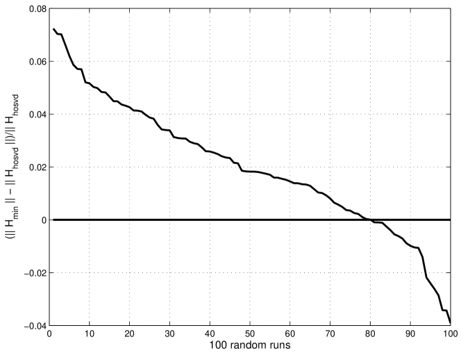
In about 80% of the runs the minimal Krylov method generated better approximations than the truncated HOSVD, but the difference was quite small.

In the following experiment we compared the performance of different variants of the optimized minimal Krylov recursion applied to sparse tensors. We generated tensors based on Facebook graphs for different US universities [29]. The Caltech graph is represented by a $597\times 597$ sparse matrix. For each individual there is housing information. Using this we generated a tensor of dimension $597\times 597\times 64$, with 25646 nonzeros. The purpose was to see how good approximations the different methods gave as a function of the subspace dimension. We compared the minimal Krylov recursion to the following optimized variants:

Opt-HOSVD. The minimal Krylov recursion with optimization based on HOSVD of the core tensor (30). This variant is very costly and is included only as a benchmark.

Opt-Krylov. The minimal Krylov recursion that utilized three inner Krylov steps to obtain approximations to the optimized linear combinations. This is an implementation of the discussion from the second part of Section 4.3.

Opt-Alg8. Algorithm 8 in [11].

Truncated HOSVD. This was included as a benchmark comparison.

minK-back. In this method we used the minimal Krylov method but performed 10 extra steps. Then we formed the core $\mathcal{H}$ and computed a truncated HOSVD approximation of $\mathcal{H}$. As a last step we truncated the Krylov subspaces accordingly.

In all Krylov-based methods we used four initial minimal Krylov steps before we started using the optimizations.

Figure 2: Errors in the low rank approximations of the sparse Caltech (top) and Princeton (bottom) tensors.

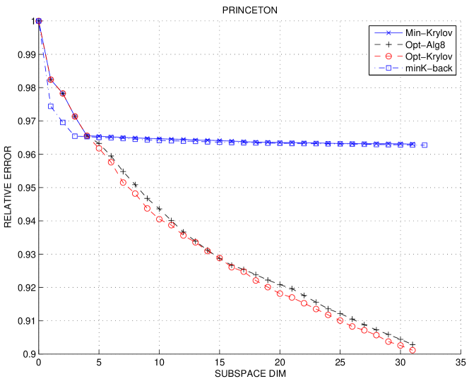
Another sparse tensor was created using the Facebook data from Princeton. Here the tensor was constructed using a student/faculty flag as third mode, giving a $6593\times 6593\times 29$ tensor with 585,754 non-zeros.

The results are illustrated in Figure 2. We see that for the Caltech tensor the “backward-looking” variant (minK-back) gives good approximations for small dimensions as long as there is a significant improvement in each step of the minimal Krylov recursion. After some ten steps all optimized variants give approximations that are rather close to that of the HOSVD.

For the Princeton tensor we only ran the minimal Krylov recursion and two of the optimizations. Here the optimized versions continued to give significant improvements as the dimension is increased, in spite of the poor performance of the minimal Krylov procedure itself.

5.2 Test on Handwritten Digits

Tensor methods for the classification of handwritten digits are described in [24, 25]. We have performed tests using the handwritten digits from the US postal service database. Digits from the database were formed into a tensor $\mathcal{D}$ of dimensions $400\times 1194\times 10$. The first mode of the tensor represents pixels, the second mode represents the variation within the different classes and the third mode represents the different classes. Our goal was to find low dimensional subspaces $U_{p}$ and $V_{q}$ in the first and second mode, respectively. The approximation of the original tensor can be written as

$$\mathbb{R}^{400\times 1194\times 10}\ni\mathcal{D}\approx\bm{\left(}U_{p},V_{q}\bm{}_{1,2}\bm{\cdot}\mathcal{F}\equiv\mathcal{D}_{p,q,10}.$$ (37)

An important difference compared to the previous sections is that here we wanted to find only two of three matrices. The class mode of the tensor was not reduced to lower rank, i.e. we were computing a rank-$(p,q,10)$ approximation of $\mathcal{D}$. We computed low rank approximations for this tensor using five different methods: (1) truncated HOSVD; (2) modified minimal Krylov recursion; (3) contracted tensor product Krylov recursion; (4) maximal Krylov recursion; and (5) optimized minimal Krylov recursion. Figure 3 shows the obtained results for low rank approximations with $(p,q)=\{(5,10),\;(10,20),\;(15,30),\;\cdots\;,\;(50,100)\}$. The reduction of dimensionality in two modes required special treatment for several of the methods. We will describe each case separately. In each case the low rank approximation $\mathcal{D}_{p,q,10}$ is given by

$$\mathcal{D}_{p,q,10}=\bm{\left(}U_{p}U_{p}^{\sf T},V_{q}V_{q}^{\sf T}\bm{}_{1,2}\bm{\cdot}\mathcal{D}$$ (38)

where the matrices $U_{p}$ and $V_{q}$ were obtained using different methods.

Truncated HOSVD

We computed the HOSVD $\mathcal{D}=\bm{\left(}U,V,W\bm{}\bm{\cdot}\mathcal{C}$ and truncated the multilinear singular matrices, i.e. $U_{p}=U(:,1:p)$ and $V_{q}=V(:,1:q)$.

Modified minimal Krylov recursion

The minimal Krylov recursion was modified in several respects. We ran Algorithm 4 for 10 iterations and obtained $U_{10},V_{10},W_{10}$. Next we ran $p-10$ iterations and generated only $u$ and $v$ vectors. For every new $u_{k+1}$ we used $\bar{v}$ and $\bar{w}$ as random liner combination of vectors in $V_{k}$ and $W_{10}$, respectively. In the last $q-p$ iterations we only generated new $v$ vectors using again random linear combinations of vectors in $U_{p}$ and $W_{10}$.

Contracted tensor product Krylov recursion

For this method we applied $p$ and $q$ steps of the Lanczos method with random starting vectors on the matrices $\left\langle\mathcal{A},\mathcal{A}\right\rangle_{-1}$ and $\left\langle\mathcal{A},\mathcal{A}\right\rangle_{-2}$, respectively.

Maximal Krylov recursion

We used the maximal Krylov recursion with starting vectors $u_{1}$ and $v_{1}$ to generate $W_{1}\rightarrow U_{2}\rightarrow V_{3}\rightarrow W_{6}\rightarrow U_{19}\rightarrow V_{115}$. Clearly, we now need to make modification to the general procedure. $W_{10}$ was obtained as the third mode singular matrix from the HOSVD of the product $\mathcal{D}\bm{\cdot}\bm{\left(}U_{19},V_{115}\bm{}_{1,2}$ and as a last step we computed $U_{100}$ as the 100 dimensional dominant subspace obtained from the first mode singular matrix of $\mathcal{D}\bm{\cdot}\bm{\left(}V_{114},W_{10}\bm{}_{2,3}$. The $U_{p}$ and $V_{q}$ used for the approximation in (38) were constructed as follows: We formed the product $\bar{\mathcal{C}}=\mathcal{D}\bm{\cdot}\bm{\left(}U_{100},V_{115}\bm{}_{1,2}$ and computed the HOSVD $\bm{\left(}\tilde{U},\tilde{V},\tilde{W}\bm{}\bm{\cdot}\tilde{\mathcal{C}}=\bar{\mathcal{C}}$. Then $U_{p}=U_{100}\tilde{U}(:,1:p)$ and $V_{q}=U_{115}\tilde{V}(:,1:q)$.

Optimized minimal Krylov recursion

For this minimal Krylov recursion we used the optimization approach, for every new vector, from the first part of Section 4.3. The coefficients for the linear combinations were obtained by best rank-$(1,1,1)$ approximation of factors as $\mathcal{C}_{w}$ in Equation (30).

Figure 3: The relative error of the low rank approximations obtained using five different methods. The $x$-axis indicates the ranks $(p,q,10)=(p,2p,10)$ in the approximation.

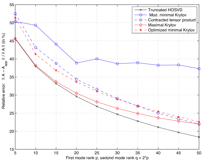
The experiments with the handwritten digits are illustrated in Figure 3. We made the following observations: (1) The truncated HOSVD give the best approximation for all cases; (2) The minimal Krylov approach did not perform well. We observed several breakdowns for this methods as the ranks in the approximation increased. Every time the process broke down we used a randomly generated vector that was orthonormalized against all previously generated vectors. (3) The Lanczos method on the contracted tensor products performed very similar as the optimized minimal Krylov method. (4) The performance of the maximal Krylov method was initially as good as the truncated HOSVD but its performance degraded eventually.

Classifications results using these subspaces in the algorithmic setting presented in [25] are similar for all methods, indicating that all of the methods capture subspaces that can used for classification purposes.

5.3 Tests on the Netflix Data

A few years ago, the Netflix company announced a competition to improve their algorithm for movie recommendations. Netflix made available movie ratings from 480,189 users/costumers on 17,770 movies during a time period of 2243 days. In total there were over 100 million ratings. We will not address the Netflix problem, but we will use the data to test some of the Krylov methods we are proposing. For our experiments we formed the tensor $\mathcal{A}$ that is $480,189\times 17,770\times 2243$ and contains all the movie ratings. Entries in the tensor for which we do not have any rating were considered as zeros. We used the minimal Krylov recursion and the Lanczos process on the products $\left\langle\mathcal{A},\mathcal{A}\right\rangle_{-1}$, $\left\langle\mathcal{A},\mathcal{A}\right\rangle_{-2}$ and $\left\langle\mathcal{A},\mathcal{A}\right\rangle_{-3}$ to obtain low rank approximations of $\mathcal{A}$.

In Figure 4 (left plot) we present the norm of the approximation, i.e. $\|\mathcal{A}_{\text{min}}\|=\|\mathcal{C}_{\text{min}}\|$, where $\mathcal{C}_{\text{min}}=\mathcal{A}\bm{\cdot}\bm{\left(}U_{k},V_{k},W_{k}\bm{}$. We have the same low rank approximation in each mode and the ranks range from $k=5,10,15,\dots,100$. The plot contains three different runs with random initial vectors in all three modes and a fourth curve that is initiated with the means of the first, second and third mode fibers. Observe that for this size of tensors it is practically impossible to form the approximation $\mathcal{A}_{\text{min}}=\bm{\left(}U_{k}U_{k}^{\sf T},V_{k}V_{k}^{\sf T},W_{k}W_{k}^{\sf T}\bm{}\bm{\cdot}\mathcal{A}$ since the approximation will be dense. But the quantity $\|\mathcal{C}_{\text{min}}\|$ is computable and indicates the quality of the approximation. Larger $\|\mathcal{C}_{\text{min}}\|$ means better approximation. In fact for orthonormal matrices $U,V,W$ it holds that $\|\mathcal{C}_{\text{min}}\|\leq\|\mathcal{A}\|$.

Figure 4: We plot $\|\mathcal{C}_{\text{min}}\|$ as a function of the rank $(p,q,r)=(p,p,p)$ in the approximation with $p=5,10,15,\dots,100$. Left plot: $U_{p},V_{p},W_{p}$ are obtained using the minimal Krylov recursion. Four runs are presented: one using starting vectors $u_{1},v_{1},w_{1}$ as the means of the mode one, two and three fibers of $\mathcal{A}$ and three runs with different set of random initial vectors. Right plot: The subspaces for his case were obtained from separate Lanczos recurrences of contracted tensor products. The starting vectors were chosen as in the left plot.

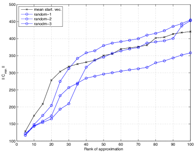
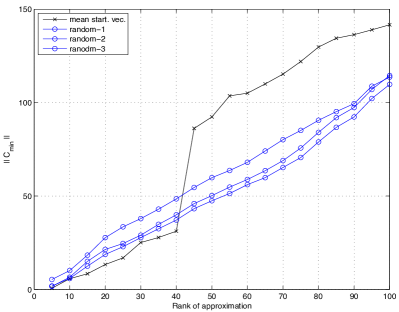
Figure 4 (right plot) contains similar plots, but now the approximating matrices $U_{k},V_{k},W_{k}$ are obtained using the Lanczos process on the symmetric matrices $\left\langle\mathcal{A},\mathcal{A}\right\rangle_{-1}$, $\left\langle\mathcal{A},\mathcal{A}\right\rangle_{-2}$ and $\left\langle\mathcal{A},\mathcal{A}\right\rangle_{-3}$. We never formed the first two products, but use the computational formula from Equation (32) for obtaining first mode vectors and a similar one for obtaining second mode vectors. We did form $\left\langle\mathcal{A},\mathcal{A}\right\rangle_{-3}$ explicitly since it is a relatively small matrix. We ran the Lanczos process with ranks $k=5,10,15,\dots,100$ using random starting vectors in all three modes. Three tests were made and we used the Lanczos vectors in $U_{k},V_{k},W_{k}$. In addition we computed the top 100 eigenvectors for each one of the contracted products.

We remark that this Netflix tensor is special in the sense that every third mode fibre, i.e. $\mathcal{A}(i,j,:)$, contains only one nonzero entry. It follows that the product $\left\langle\mathcal{A},\mathcal{A}\right\rangle_{-3}$ is a diagonal matrix. Our emphasis for these tests was to show that the proposed tensor Krylov methods can be employed on very large and sparse tensors.

In this experiment it turned out to be more efficient to store the sparse Netflix tensor slice-wise, where each slice itself was a sparse matrix, than using the sparse tensor format from the TensorToolbox.

6 Conclusions and Future Work

In this paper we propose several ways to generalize matrix Krylov methods to tensors, having applications with sparse tensor in mind. In particular we introduce three different methods for tensor approximations. These are the minimal, maximal Krylov methods and the contracted tensor product methods. We prove that, given a tensor of the form $\mathcal{A}=\bm{\left(}X,Y,Z\bm{}\bm{\cdot}\mathcal{C}$ with $\operatorname{rank}(\mathcal{A})=\operatorname{rank}(\mathcal{C})=(p,q,r)$, a modified version of the minimal Krylov recursion extracts the associated subspaces of $\mathcal{A}$ in $\max\{p,q,r\}$ iterations. We also investigate a variant of the the optimized minimal Krylov recursion [11], which gives better approximation than the minimal recursion, and which can be implemented using only sparse tensor operations. We also show that the maximal Krylov approach generalizes the matrix Krylov factorization to a corresponding tensor Krylov factorization.

The experiments clearly indicate that the Krylov methods are useful for low-rank approximation of large and sparse tensors. In [11] it is also shown that they are efficient for further compression of dense tensors that are given in canonical format. The tensor Krylov methods can also be used to speed up HOSVD computations.

As the research on tensor Krylov methods is still in a very early stage, there are numerous questions that need to be answered, and which will be the subject of our continued research. We have hinted to some in the text; here we list a few others.

1. Details with respect to detecting true break down, in floating point arithmetic, and distinguishing those from the case when a complete subspaces is obtained need to be worked out.

2. A difficulty with Krylov methods for very large problems is that the basis vectors generated are in most cases dense. Also, when the required subspace dimension is comparatively large, the cost for (re)orthogonalization will be high. For matrices the subspaces can be improved using the implicitly restarted Arnoldi (Krylov-Schur) approach [21, 28]. Preliminary tests indicate that similar procedures for tensors may be efficient. The properties of such methods and their implementation will be studied.

3. The efficiency of the different variants of Krylov methods in terms of the number of tensor-vector-vector operations, and taking into account the convergence rate will be investigated.

References

- Bader et al. [2006] Bader, B. W., Harshman, R. A., Kolda, T. G., 2006. Temporal analysis of social networks using three-way DEDICOM. Tech. Rep. SAND2006-2161, Sandia National Laboratories, Albuquerque, NM.
- Bader et al. [2007] Bader, B. W., Harshman, R. A., Kolda, T. G., October 2007. Temporal analysis of semantic graphs using ASALSAN. In: ICDM 2007: Proceedings of the 7th IEEE International Conference on Data Mining. pp. 33–42.
- Bader and Kolda [2006] Bader, B. W., Kolda, T. G., 2006. Algorithm 862: MATLAB tensor classes for fast algorithm prototyping. ACM Trans. Math. Softw. 32 (4), 635–653.
-
Bader and Kolda [2007]
Bader, B. W., Kolda, T. G., 2007. Efficient MATLAB computations with sparse
and factored tensors. SIAM Journal on Scientific Computing 30 (1), 205–231.
URL http://link.aip.org/link/?SCE/30/205/1 - Carroll and Chang [1970] Carroll, J. D., Chang, J. J., 1970. Analysis of individual differences in multidimensional scaling via an n-way generalization of Eckart-Young decomposition. Psychometrika 35, Psychometrika.
- Chew et al. [2007] Chew, P. A., Bader, B. W., Kolda, T. G., Abdelali, A., 2007. Cross-language information retrieval using PARAFAC2. In: KDD ’07: Proceedings of the 13th ACM SIGKDD International Conference on Knowledge Discovery and Data Mining. ACM Press, pp. 143–152.
De Lathauwer et al. [2000]
De Lathauwer, L., Moor, B. D., Vandewalle, J., 2000. A multilinear singular
value decomposition. SIAM J. on Matrix Anal. Appl. 21 (4), 1253–1278.
URL http://link.aip.org/link/?SML/21/1253/1 -
De Silva and Lim [2008]
De Silva, V., Lim, L.-H., 2008. Tensor rank and the ill-posedness of the best
low-rank approximation problem. SIAM J. on Matrix Anal. Appl. 30 (3),
1084–1127.
URL http://link.aip.org/link/?SML/30/1084/1 - Eldén and Savas [2009] Eldén, L., Savas, B., 2009. A Newton–Grassmann method for computing the best multi-linear rank-() approximation of a tensor. SIAM J. Matrix Anal. Appl. 31, 248–271.
- Golub and Kahan [1965] Golub, G. H., Kahan, W., 1965. Calculating the singular values and pseudo-inverse of a matrix. SIAM J. Numer. Anal. Ser. B 2, 205–224.
- Goreinov et al. [2010] Goreinov, S., Oseledets, I., Savostyanov, D., April 2010. Wedderburn rank reduction and Krylov subspace method for tensor approximation. Part 1: Tucker case. Tech. Rep. Preprint 2010-01, Inst. Numer. Math., Russian Academy of Sciences.
- Harshman [1970] Harshman, R. A., 1970. Foundations of the PARAFAC procedure: Models and conditions for an ”explanatory” multi-modal factor analysis. UCLA Working Papers in Phonetics 16, 1–84.
- Hitchcock [1927] Hitchcock, F. L., 1927. Multiple invariants and generalized rank of a p-way matrix or tensor. J. Math. Phys. Camb. 7, 39–70.
- Ishteva et al. [2009] Ishteva, M., De Lathauwer, L., Absil, P.-A., Van Huffel, S., 2009. Best low multilinear rank approximation of higher-order tensors, based on the Riemannian trust-region scheme. Tech. Rep. 09-142, ESAT-SISTA, K.U.Leuven (Leuven, Belgium).
- Jessup and Martin [2001] Jessup, E. R., Martin, J. H., 2001. Taking a new look at the latent semantic analysis approach to information retrieval. In: Berry, M. W. (Ed.), Computational Information Retrieval. SIAM, Philadelphia, PA, pp. 121–144.
Khoromskij and Khoromskaia [2009]
Khoromskij, B. N., Khoromskaia, V., 2009. Multigrid accelerated tensor
approximation of function related multidimensional arrays. SIAM Journal on
Scientific Computing 31 (4), 3002–3026.
URL http://link.aip.org/link/?SCE/31/3002/1 - Kobayashi and Nomizu [1963] Kobayashi, S., Nomizu, K., 1963. Foundations of Differential Geometry. Interscience Publisher.
- Kolda et al. [2005] Kolda, T. G., Bader, . W., Kenny, J. P., November 2005. Higher-order web link analysis using multilinear algebra. In: ICDM 2005: Proceedings of the 5th IEEE International Conference on Data Mining. pp. 242–249.
Kolda and Bader [2006]
Kolda, T. G., Bader, B. W., 2006. The TOPHITS model for higher-order web link
analysis. In: Proceedings of the SIAM Data Mining Conference Workshop on Link
Analysis, Counterterrorism and Security.
URL http://www.siam.org/meetings/sdm06/workproceed/Link%20A%nalysis/21Tamara_Kolda_SIAMLACS.pdf -
Kolda and Bader [2009]
Kolda, T. G., Bader, B. W., 2009. Tensor decompositions and applications. SIAM
Review 51 (3), 455–500.
URL http://link.aip.org/link/?SIR/51/455/1 - Lehoucq et al. [1998] Lehoucq, R., Sorensen, D., Yang, C., 1998. Arpack Users’ Guide: Solution of Large Scale Eigenvalue Problems with Implicitly Restarted Arnoldi Methods. SIAM, Philadelphia.
Lohr [2009, September, 21]
Lohr, S., 2009, September, 21. A $1 million research bargain for netflix, and
maybe a model for others. The New York Times.
URL http://www.nytimes.com/2009/09/22/technology/internet/2%2netflix.html?_r=1 -
Oseledets et al. [2008]
Oseledets, I. V., Savostianov, D. V., Tyrtyshnikov, E. E., 2008. Tucker
dimensionality reduction of three-dimensional arrays in linear time. SIAM
Journal on Matrix Analysis and Applications 30 (3), 939–956.
URL http://link.aip.org/link/?SML/30/939/1 - Savas [2003] Savas, B., 2003. Analyses and tests of handwritten digit recognition algorithms. Master’s thesis, Linköping University, http://www.mai.liu.se/~besav/.
- Savas and Eldén [2007] Savas, B., Eldén, L., 2007. Handwritten digit classification using higher order singular value decomposition. Pattern Recognition 40, 993–1003.
- Savas and Lim [2010] Savas, B., Lim, L.-H., 2010. Quasi-Newton methods on Grassmannians and multilinear approximations of tensors. Submitted to SIAM Journal on Scientific Computing.
- Stewart [2001] Stewart, G. W., 2001. Matrix Algorithms II: Eigensystems. SIAM, Philadelphia.
Stewart [2002]
Stewart, G. W., 2002. A Krylov–Schur algorithm for large eigenproblems. SIAM
Journal on Matrix Analysis and Applications 23 (3), 601–614.
URL http://link.aip.org/link/?SML/23/601/1 - Traud et al. [2008] Traud, A. L., Kelsic, E. D., Mucha, P. J., Porter, M. A., 2008. Community structure in online collegiate social networks. Tech. rep., arXiv:physics.soc-ph/0809.0690.
- Tucker [1964] Tucker, L. R., 1964. The extension of factor analysis to three-dimensional matrices. Contributions to Mathematical Psychology, 109–127.
- Vasilescu and Terzopoulos [2002] Vasilescu, M. A. O., Terzopoulos, D., 2002. Multilinear analysis of image ensembles: Tensorfaces. In: Proc. 7th European Conference on Computer Vision (ECCV’02). Lecture Notes in Computer Science, Vol. 2350. Springer Verlag, Copenhagen, Denmark, pp. 447–460.