Using microlensed quasars to probe the structure of the Milky Way

Abstract

This paper presents an investigation into the gravitational microlensing of quasars by stars and stellar remnants in the Milky Way. We present predictions for the all-sky microlensing optical depth, time-scale distributions and event rates for future large-area sky surveys. As expected, the total event rate increases rapidly with increasing magnitude limit, reflecting the fact that the number density of quasars is a steep function of magnitude. Surveys such as Pan-STARRS and LSST should be able to detect more than ten events per year, with typical event durations of around one month. Since microlensing of quasar sources suffers from fewer degeneracies than lensing of Milky Way sources, they could be used as a powerful tool for recovering the mass of the lensing object in a robust, often model-independent, manner. As a consequence, for a subset of these events it will be possible to directly ‘weigh’ the star (or stellar remnant) that is causing the lensing signal, either through higher order microlensing effects and/or high-precision astrometric observations of the lens star (using, for example, Gaia or SIM-lite). This means that such events could play a crucial role in stellar astronomy. Given the current operational timelines for Pan-STARRS and LSST, by the end of the decade they could potentially detect up to 100 events. Although this is still too few events to place detailed constraints on Galactic models, consistency checks can be carried out and such samples could lead to exciting and unexpected discoveries.

1 Introduction

Gravitational microlensing is now established as a powerful tool for various aspects of Galactic science. The concept of gravitational microlensing, where a background object is temporarily brightened by the gravitational lensing effect of a passing foreground object, is believed to have been initially conceived by Einstein around 1912 (Renn, Sauer & Stachel, 1997). As he stated in a later publication (Einstein, 1936), his opinion was that ”there is no great chance of observing this phenomenon”. Fortunately the idea was later resurrected by several authors (Liebes, 1964; Refsdal, 1964), in particular Paczyński (1986). Following the proposal of Paczyński, many experiments began to hunt for microlensing events towards the Galactic bulge and the Magellanic Clouds: OGLE (Udalski et al., 1992), EROS (Aubourg et al., 1993), MACHO (Alcock et al., 1993), MOA (Bond et al., 2001). To date thousands of microlensing events have been detected toward several directions, including the Galactic bulge (Thomas et al., 2005; Sumi et al., 2006; Hamadache et al., 2006), Magellanic Clouds (Tisserand et al., 2007; Wyrzykowski et al., 2009, 2010), and M31 (Calchi Novati et al., 2005; de Jong et al., 2006) and even in surveys of bright nearby stars (Fukui et al., 2007; Gaudi et al., 2008).

The purpose of this paper is to deal with a previously under-exploited set of targets, namely quasars. Although quasar microlensing has been observed for many years (e.g. Chang & Refsdal, 1979; Irwin et al., 1989; Anguita et al., 2008) this has, with a few exceptions (e.g. Byalko, 1970), almost exclusively been lensing of background quasars by compact objects in the intervening (strong) lensing galaxy. In contrast, we are interested in the lensing of background quasars by stars in the Milky Way. This is a particularly prescient subject because imminent large-scale optical surveys, such as Pan-STARRS (Kaiser et al., 2002) and LSST (Tyson, 2002; Ivezić et al., 2008), will monitor the whole available sky every few nights down to magnitudes which are sufficient to monitor several million background quasars. If large enough samples of such microlensing events could be accrued then it will be possible to use them to constrain models of the Galaxy.

One reason why quasars are potentially important targets is that they break a number of the degeneracies known to inhibit the analysis of microlensing events from sources within our own Galaxy. In general, for lensing of Galactic sources it is difficult to determine the properties of the lensing population because all of the information about the event is contained in one observable, namely the event time-scale. As a consequence, there are a number of degeneracies which need to be broken in order to determine, for example, the lens mass or distance. For sources within the Milky Way, in general, we do not know the distance or transverse velocity of the star which is lensed. For quasars the interpretation is made significantly easier because we can assume that the source is at infinity and that the transverse velocity is negligible. In this case the lens mass is simply a function of the (known) time-scale and the (unknown) lens distance and velocity,

$$M\approx 0.3\rm\rm M_{\odot}\left({t_{\rm E}\over 30~{}\rm day}\right)^{2}\left({D_{\rm L}\over 4~{}\rm kpc}\right)\left({\mu_{t}\over 9.4~{}\rm mas~{}yr^{-1}}\right)^{2},$$ (1)

where $D_{\rm L}$ and $\mu_{t}$ are the lens distance and proper motion, respectively, and $t_{\rm E}$ is the event time-scale. This makes the interpretation of quasar microlensing events significantly easier than that of Galactic sources and opens up the possibility of carrying out model-independent mass determinations using high precision astrometry from, for example, ESA’s Gaia mission (Perryman et al., 2001). Even without a measurement of the lens distance/velocity, it could also be possible to use higher-order microlensing effects such as the microlensing parallax (Gould, 1992) to break the degeneracy. Clearly quasar microlensing has the potential to become an important avenue for probing both stellar and Galactic astrophysics.

In this paper we carry out Monte Carlo simulations to address this issue, presenting an all-sky prediction of the rate and optical depth of microlensed quasars. The paper is organised as follows. In Section 2, we describe the model and theory. In Section 3, we present the main results, dealing with the time-scale distribution (3.1), the predictions for the optical depth and event rate (3.2) and also the prospects for determining the lens masses (3.3). We present a summary and discussion in Section 4.

2 The Model

We utilise a Monte Carlo simulation to give an estimate of the rate and optical depth for microlensed quasar events. The details of the simulation are described in the following subsections. Our microlensing model is constructed following Kiraga & Paczyński (1994) and is similar to a number of previous works (Wood & Mao, 2005; Han, 2008).

2.1 Stellar distribution

In this work we want to obtain an all sky estimate of microlensed quasars by the Milky Way stars, which requires a model for the stellar mass distribution. To do this we follow the model of Binney & Tremaine (2008, hereafter BT08). Unless otherwise stated all parameters are taken from Model I in table 2.3 of BT08 and the solar radius is taken to be 8 kpc. It is immediately clear that the stellar halo’s contribution is negligible. Thus, only bulge and disc stars are considered in this paper.

The bulge is treated as a bar with its longest axis inclined by about $20^{\circ}$ to the line from Sun to the Galactic center and the stellar mass distribution in the bar is given by

$$\rho_{\rm bar}(R,z)=\rho_{\rm bar,0}\left({s\over a_{\rm bar}}\right)^{-\alpha_{\rm bar}}e^{-s^{2}/r_{\rm bar}^{2}},$$ (2)

where $s=\sqrt{x^{2}+(y^{2}+z^{2})/q^{2}}$. The bulge is truncated at a radius $r_{\rm bar}$. The three dimension Cartesian coordinates ($x$, $y$, and $z$) are shown in Fig. 1. For the bar parameters we adopt $a_{\rm bar}=1~{}\rm kpc$, $\alpha_{\rm bar}=1.8$, $q=0.35$, $r_{\rm bar}=\rm 3~{}kpc$, and $\rho_{\rm bar,0}=1.22~{}\rm\rm M_{\odot}/pc^{3}$. We have set the normalisation of the bar mass so that the bar has the same mass as the original bulge ($0.518\times 10^{10}\rm\rm M_{\odot}$).

The disc is modeled as the sum of two double-exponentials, which correspond to the thin- and thick-disc components. The Galactic disc density distribution in cylindrical coordinates is

$$\rho_{\rm disc}(R,z)=\Sigma_{\rm disc}e^{-R/R_{\rm disc}}\left({\alpha_{0}\over 2z_{0}}e^{-|z|/z_{0}}+{\alpha_{1}\over 2z_{1}}e^{-|z|/z_{1}}\right),$$ (3)

where $\Sigma_{\rm disc}=1773.12~{}\rm\rm M_{\odot}/pc^{2}$ is the central surface density, $R$ is the radial distance, $R_{\rm disc}=2~{}\rm kpc$ is the disc scale-length (both components are assumed to have the same scale-length), $z_{0}=0.3~{}\rm kpc$, and $z_{1}=1.0~{}\rm kpc$ are the scale-heights for the thin and thick components, respectively, and $\alpha_{0}=0.9333$ and $\alpha_{1}=0.0667$ are the respective normalisations. The total mass of the disc in this model is $5.13\times 10^{10}{\rm\rm M_{\odot}}$.

2.2 Lens Mass Function

For the mass function we use the four part power-law distribution model of Kroupa (2002),

$$\xi_{0}(M)\equiv{dN\over dM}=k\cases{0.4687M^{-0.3}&$0.01\leq M/\rm M_{\odot}<0.08$,\cr 0.0375M^{-1.3}&$0.08\leq M/\rm M_{\odot}<0.5$,\cr 0.0187M^{-2.2}&$0.5\leq M/\rm M_{\odot}<1.0$,\cr 0.0187M^{-2.7}&$1.0\leq M/\rm M_{\odot}<120$.\cr}$$ (4)

The normalisation $k$ is obtained through the integral,

$$\int_{0.01}^{120}M\xi_{0}(M)dM=\rho_{\rm disc,solar},$$ (5)

where $\rho_{\rm disc,solar}$ is the stellar density in the solar neighbourhood (which can be derived from equation 3). We find that $k=0.762~{}\rm M_{\odot}^{-1}\>pc^{-3}$. Note that unlike some previous authors we do not adopt different mass functions for different populations; as argued by Bastian, Covey & Meyer (2010), there is no clear evidence to support strong variations in the initial mass function.

We invoke the following simple approach for dealing with stellar evolution. The objects with initial masses $0.01\sim 0.08~{}\rm M_{\odot}$ and $0.08\sim 1.0~{}\rm M_{\odot}$ are assumed to become brown dwarfs and main-sequence stars, respectively. The stars with initial mass $1.0\sim 8.0~{}\rm M_{\odot}$ are assumed to evolve into $0.6~{}\rm M_{\odot}$ white dwarfs. The stars with $8.0\sim 40.0~{}\rm M_{\odot}$ are assumed to evolve into $1.35~{}\rm M_{\odot}$ neutron stars, and more massive stars are assumed to evolve into $5.0~{}\rm M_{\odot}$ black holes.

We assume that the lens number density is proportional to the stellar mass density given in equations (2) and (3) (i.e. $n\propto\rho_{\rm bar}+\rho_{\rm disc}$). For convenience, we rewrite the total stellar distribution equation as follows,

$$\rho_{\rm total}=\rho_{\rm bar}+\rho_{\rm disc}=\rho_{\rm disc,solar}\chiup(l,b,D_{\rm L}).$$ (6)

From this we can deduce the lens number density within a mass range, $M$, $M+dM$ and a velocity range $v$, $v+dv$, as follows,

$$n(l,b,D_{\rm L},M,v_{l},v_{b})=\chiup(l,b,D_{\rm L})\xi_{0}(M)f(v_{l},v_{b}).$$ (7)

where $l,~{}b$ are the galactic coordinates and $D_{\rm L}$ is the distance to the lens, $\xi_{0}$ is the lens mass function given in equation (4) and $\chiup(l,b,D_{\rm L})$ is the dimensionless mass distribution (see equation 6).

2.3 Lens luminosity

In addition to the lens mass, we also consider the lens luminosity. This allows us to investigate the possibility of detecting the lenses and measuring their proper motion and distance, which will break the degeneracy in equation (1) and allow a model-independent measurement of the lens mass.

For the main-sequence stars we estimate the lens brightness using the mass-luminosity relation of Cox (1998), while we assume that all non-main-sequence lenses are dark. The mass-luminosity relation of Cox (1998) is given in the $V$-band in the Johnson-Cousins $UBVRI$ system. In order to compare with LSST observations (see Section 2.6) we need to transform the $V$-band luminosity into a luminosity in the LSST $ugrizy$ photometry system. To do this we use the empirical colour transformations given by Jordi et al (2006).

As the lenses are distributed at different distances from the Sun, we need to carefully consider the Galactic dust extinction. To do this we utilise the Galactic dust map of Schlegel et al. (1998, hereafter SFD), combining this with a model of the interstellar medium from BT08, as follows. We first construct a model to calculate the total extinction along a given line-of-sight for the photometric band $x$,

$$A_{x}\left({\infty}\right)=k_{x}\int_{0}^{\infty}\rho_{g}dl,$$ (8)

where $k_{x}$ is a constant (i.e. this does not vary across the sky) and the distribution of the interstellar medium ($\rho_{g}$) is modelled using equation (2.211) of BT08. We estimate $k_{x}$ by carrying out a least-squared fit between $A_{x}\left({\infty}\right)$ and the observed value of the total extinction from SFD using $10^{6}$ lines-of-sight uniformly distributed across the sky. Once we have estimated $k_{x}$ we can calculate the extinction that a lens is subject to using the following formula,

$$A_{x}\left({D_{\rm L}}\right)=k_{x}\int_{0}^{D_{\rm L}}\rho_{g}dl.$$ (9)

2.4 Velocity Distribution

To calculate the event rate we need to know the velocities of the observer, lenses and sources. For simplicity we neglect the motion of the Earth around the Sun, the so-called parallax effect (Gould, 1992), returning to this briefly in Section 3.3. For the calculation of microlensing event rate only the relative lens-source transverse velocity (i.e. the transverse velocity of the lens, in the lens-plane, relative to the observer-source line of sight), $\textbf{v}_{t}$, is needed, which can be written,

$$\textbf{v}_{t}\approx\textbf{v}_{\rm L}-\textbf{v}_{O}~{}~{}~{}{\rm for}~{}~{}D_{\rm L}\ll D_{\rm S},$$ (10)

where $D_{\rm L}$ and $D_{\rm S}$ are the distances to the lens and source, respectively, and $\textbf{v}_{\rm O}$ and $\textbf{v}_{\rm L}$ are the components of the velocity tangential to the line-of-sight for the observer and lens, respectively

We model the velocity distributions of the lens stars in the Milky Way using Gaussian distributions, adopting the Solar motion with respect to the local standard of rest from Schönrich, Binney & Dehnen (2010). We take two separate tri-variate Gaussians for the thin and thick discs, using the means and dispersions from table 2 of Smith et al. (2007). For the bar stars, the random velocities are assumed to have Gaussian distributions with $(\sigma_{x^{\prime\prime}},\sigma_{y^{\prime\prime}},\sigma_{z^{\prime\prime}})=(113.6,~{}77.4,~{}66.3)~{}\rm km~{}\rm s^{-1}$ (Han & Gould, 1995) along the three axes of the bar. Here, the coordinates $(x^{\prime\prime},~{}y^{\prime\prime},~{}z^{\prime\prime})$ are centred at the Galactic centre; $x^{\prime\prime}$ represents the longest axis of the bar, $z^{\prime\prime}$ is directed towards the north Galactic pole. The bar velocity dispersion needs to be computed in the Galactocentric cylindrical coordinate system by,

$$\sigma_{R,\rm bar}^{2} = \sigma_{x}^{2}\;{\rm cos}^{2}\varphiup~{}+~{}\sigma_{y}^{2}\;{\rm sin}^{2}\varphiup,$$ (11)

$$~{}\sigma_{\varphiup,\rm bar}^{2} = \sigma_{x}^{2}\;{\rm sin}^{2}\varphiup~{}+~{}\sigma_{y}^{2}\;{\rm cos}^{2}\varphiup,$$ (12)

$$\sigma_{z,\rm bar}^{2} = \sigma_{z}^{2},$$ (13)

where $(\sigma_{x},\sigma_{y},\sigma_{z})=(110.0,~{}82.5,~{}66.3)~{}\rm km~{}\rm s^{-1}$ are the velocity dispersions along the $x,~{}y,~{}z$ axis as shown in Fig. 1, which are calculated from $(\sigma_{x^{\prime\prime}},\sigma_{y^{\prime\prime}},\sigma_{z^{\prime\prime}})$ given the assumed bar angle of $20^{\circ}$. The resultant velocity dispersion is a function of the azimuth $\varphiup$. The rotation component of the bar velocities $v_{\varphiup,\rm bar}$ are estimated following Han & Gould (1995),

$$v_{\varphiup,\rm bar}=\cases{v_{max}({R\over 1~{}\rm kpc})&$R~{}<~{}1~{}\rm kpc,~{}~{}solid~{}body~{}rotation$,\cr v_{max}&$R~{}\geq~{}1~{}\rm kpc,~{}~{}flat~{}rotation$.\cr}$$ (14)

where $v_{max}~{}=~{}100~{}\rm km~{}s^{-1}$ is adopted.

For the calculation of the relative lens-source transverse velocity, $\textbf{v}_{t}$, we need to convert the lens velocity components from Galactocentric cylindrical coordinates into solar-centric spherical coordinates. The conversion is done as follows,

$$\left({\begin{array}[]{c}v_{r}\\ v_{l}\\ v_{b}\end{array}}\right)=\left({\begin{array}[]{rrr}\sin b\cos\alpha&-\sin b\sin\alpha&\cos b\\ \sin\alpha&\cos\alpha&0\\ \cos b\cos\alpha&-\cos b\sin\alpha&-\sin b\end{array}}\right)\left({\begin{array}[]{c}v_{R}\\ v_{\varphiup}\\ v_{z}\end{array}}\right),$$ (15)

where $(v_{r},v_{l},v_{b})$ are the velocity components in solar-centric spherical coordinates corresponding to the radial, galactic longitude and galactic latitude components, respectively. The angle $\alpha$ is the angle between the lines connecting the Sun, the projected position of the lens on the Galactic plane, and the Galactic centre (see Fig. 1),which can be computed by,

$$\alpha=\sin^{-1}{R_{0}~{}\sin l/R},~{}~{}~{}~{}R=\sqrt{R_{0}^{2}+d^{2}-2R_{0}~{}d~{}\cos l},$$ (16)

where $d=D_{\rm L}~{}\sin b$.

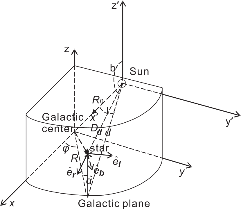
Figure 1: Position of a lens star seen from the Sun, where $(D_{\rm L},l,b)$ are the galactic coordinates of the star, $(R,\varphiup,z)$ are the Galactocentric cylindrical coordinates, and $R_{0}$ is the Galactocentric distance of the Sun. The vectors $\hat{\textbf{e}}_{r}$, $\hat{\textbf{e}}_{l}$, and $\hat{\textbf{e}}_{b}$ are the unit vectors in the solar-centric spherical coordinates.

2.5 Quasar Luminosity Function

Quasars are very energetic and distant galaxies with an active galactic nucleus. By assuming an isotropic distribution, the distribution of quasars can be given by the so called quasar luminosity function (QLF). A lot of work has been carried out on the QLF in recent years (Boyle et al., 2000; Richards et al., 2006; Fontanot et al., 2007; Hennawi et al., 2007; Richards et al., 2009; Croom et al., 2009), especially with the advent of surveys such as the Two Degree Field (2dF) and Sloan Digital Sky Survey (SDSS).

In this paper we assume that the quasars have a constant surface number density and follow the method of Li et al. (2007) to give an estimate of this number density. We utilise the $\Lambda$ cold dark matter ($\Lambda$ CDM) model in a flat universe (i.e. $\Omega_{m,0}+\Omega_{\Lambda,0}=1$) with $\Omega_{m,0}=0.3$, $\Omega_{\Lambda,0}=0.7$ and $h=0.7$, where $h$ is the Hubble constant in units of $100~{}\rm km~{}s^{-1}~{}Mpc^{-1}$. We then simply integrate the QLF in the redshift interval $z<8$ to derive the surface number density of quasars in the $i$- and $z$-bands. We denote the total surface density of quasars down to a particular limiting magnitude as $N(<i)$ and $N(<z)$ for the two photometric bands. Fig. 2 shows the resulting distributions.

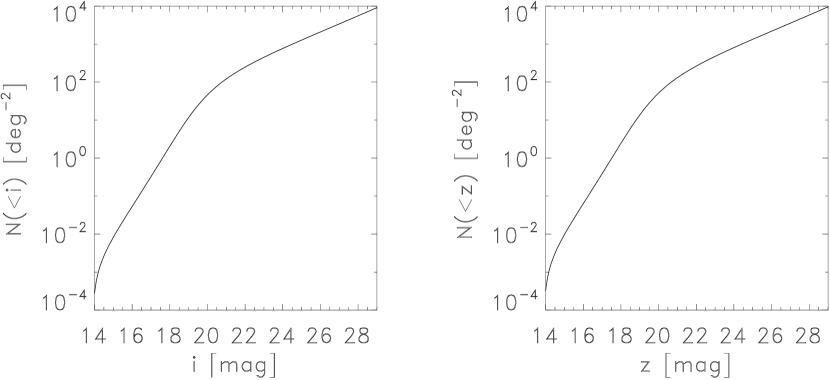
Figure 2: The surface number density of quasars as a function of limiting apparent magnitude in $i$- and $z$-bands.

Since quasars are extragalactic sources, some of the light emitted from them will be absorbed by the dust in the Milky Way. We take this into account using the extinction map of SFD. The motivation for including the $z$-band in our analysis is to see whether the reduced extinction for this longer wavelength increases the quasar microlensing event rate compared to $i$-band.

2.6 Optical Depth and Event Rate

The microlensing optical depth is defined as the probability that a particular background source falls into the Einstein radius of any foreground lens star. As has been mentioned above in Section 2.5, we assume that the quasars are distributed uniformly across the sky. If we denote the surface number density as $n_{s}(l,~{}b,~{}D_{\rm S})$, the optical depth along a given line-of-sight can be calculated following Kiraga & Paczyński (1994),

$$\tau(l,b) = {4\pi G\over c^{2}}\int_{0}^{\infty}n_{s}(l,b,D_{\rm S})D_{\rm S}^{2}dD_{\rm S}\int_{0}^{D_{\rm S}}dD_{\rm L}\chiup(l,b,D_{\rm S})D$$ (17)

$$\cdot\int_{M_{1}}^{M_{2}}M\xi_{0}(M)dM\cdot[\int_{0}^{\infty}n_{s}(l,b,D_{\rm S})D_{\rm S}^{2}dD_{\rm S}]^{-1}$$

$$\approx {4\pi G\over c^{2}}\int_{0}^{D_{\rm S}}dD_{\rm L}\chiup(l,b,D_{\rm S})D\int_{M_{1}}^{M_{2}}M\xi_{0}(M)dM,$$

where $G$ is gravitational constant, $D\equiv D_{\rm L}(D_{\rm S}-D_{\rm L})/D_{\rm S}\approx D_{\rm L}$ for $D_{\rm L}\ll D_{\rm S}$, and $M_{1}$ and $M_{2}$ are the mass limits of the lens stars. Note that the optical depth is independent of $n_{s}(l,~{}b,~{}D_{\rm S})$.

The event rate is the number of microlensing events that occur per unit time, which we again calculate following Kiraga & Paczyński (1994),

$$\Gamma(l,b) = {4\sqrt{G}\over c}\int_{0}^{\infty}dD_{\rm S}n_{s}(l,b,D_{\rm S})D_{\rm S}^{2}\int_{0}^{D_{\rm S}}dD_{\rm L}\chiup(l,b,D_{\rm L})D^{1/2}$$ (18)

$$\cdot\int_{M_{1}}^{M_{2}}dM\xi_{0}(M)M^{1/2}\iint dv_{l}dv_{b}v_{t}f(v_{l},v_{b})$$

$$\cdot[\int_{0}^{\infty}dD_{\rm S}n_{s}(l,b,D_{\rm S})D_{\rm S}^{2}]^{-1}$$

$$\approx {4\sqrt{G}\over c}\int_{0}^{D_{\rm S}}dD_{\rm L}\chiup(l,b,D_{\rm L})D^{1/2}\int_{M_{1}}^{M_{2}}dM\xi_{0}(M)M^{1/2}$$

$$\cdot\iint dv_{l}dv_{b}v_{t}f(v_{l},v_{b}).$$

The time-scale of a microlensing event, $t_{E}$, which is defined to be the time for a source to cross the Einstein radius of the lens (e.g. Mao, 2008), is given by,

$$t_{E}~{}=~{}{r_{E}\over{\rm v}_{t}}\approx~{}\frac{1}{{\rm v}_{t}}[{4GM\over c^{2}}D_{\rm L}]^{1/2}~{}~{}~{}{\rm for}~{}~{}D_{\rm L}\ll D_{\rm S}.$$ (19)

where $r_{E}$ is the physical size of the Einstein radius in the lens plane and ${\rm v}_{t}$ is the relative transverse velocity of the lens (equation 10).

During a time interval $\Delta t$, the total number of expected microlensing events is trivially,

$$N_{\rm events}=\epsilon\Gamma_{\rm total}\Delta t,$$ (20)

where $\Gamma_{\rm total}$ is the total event rate integrated over all lines-of-sight and $\epsilon$ is the detection efficiency. For simplicity, we assume $\epsilon\equiv 100$ per cent. This can be justified when one considers that the cadence of the surveys such as LSST will be of the order of a few days, which is suitable to detect practically all events in our time-scale range (see Section 3.1). We return to this issue in the following section.

3 Results

3.1 Time-Scale distributions

Using the model described above, we are able to investigate the time-scale distributions for quasar microlensing events. Fig.  3 shows the predicted event rate as a function of time-scale for the different Galactic components. The average time-scales for the bar, thin disc, thick disc and total (bar plus discs) are $31.7~{}\rm days$, $44.4~{}\rm days$, $33.3~{}\rm days$ and $41.2~{}\rm days$, respectively. The longest time-scales are obtained for thin-disc events towards $l\approx 140$ and $l\approx 210$ degrees. In these regions the mean time-scale can reach as high as 130 days; these events will be very well sampled and are likely to display microlensing parallax signatures (see Section 3.3). Note that the average time-scale for disc-lensing events reaches a minimum around the central parts of the Galaxy. The average in this region is reduced due to lenses on the far-side of the bar; these have large transverse velocities owing to their rotational velocity acting in the opposite direction to the Sun’s. The events with shortest time-scales are those caused by lenses in the Galactic bar, because bar lenses have larger velocity dispersions and hence larger transverse velocities. Furthermore, unlike nearby disc-lenses, they do not share the disc’s rotation velocity.

The combined map in the lower-panel of Fig 3 closely resembles the time-scale map for the thin disc, since the majority of events are caused by thin-disc lenses (see Section 3.2).

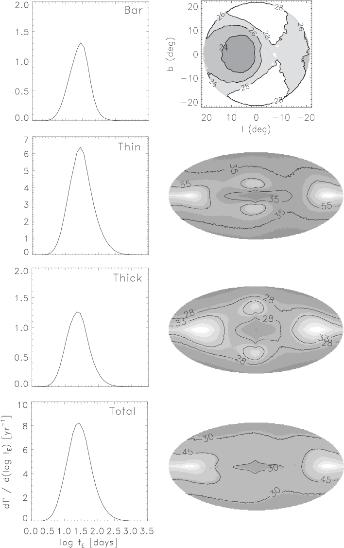
Figure 3: The left-hand panels show the predicted microlensing event rate of quasars as a function of the time-scale. The right-hand panels show the corresponding maps of the predicted average event time-scale. We show the contributions of different Galactic components, the thin-disc, the thick-disc, the bar, and the combination of bar and discs from top to bottom, respectively.

3.2 Optical Depth and Event Rate

Arguably the most important quantity which we can calculate is the total event rate, i.e. the number of events which we expect future surveys will be able to detect. This is given in Table 1 for various apparent magnitude limits. Not surprisingly the total event rate increases rapidly with increasing depth, reflecting the fact that the number density of quasars rises steeply for fainter limiting magnitudes (as shown in Fig. 2).

The contributions from the various Milky Way components are shown in Table 1. We can clearly see that the total event rate is dominated by the disc component, including the thin and thick disc components. The thick disc component contributes about $17$ per cent of the whole disc events and therefore plays a non-negligible role in quasar microlensing. Although the total mass of the thin disc is $13$ times more massive than the thick disc, the fact that the thick disc is less concentrated in regions of high extinction helps to boost its lensing signal. The bar component, with only around 10 per cent of the total mass of the disc, has significantly fewer events. As has been stated in Section 2.1, the stellar halo will have a negligible contribution.

$\Gamma$ ($yr^{-1}$)
$m_{lim}$ (mag)	Bar	Thin Disc	Thick Disc	Total
estimates for $i$-band detection
21	0.07	0.55	0.17	0.79
23	0.51	3.53	0.86	4.90
24	0.97	6.94	1.56	9.54
27	5.13	34.75	6.92	46.80
estimates for $z$-band detection
21	0.12	0.91	0.23	1.26
23	0.77	5.40	1.09	7.26
24	1.50	10.31	1.95	13.76
27	7.30	48.82	8.26	64.38

Table 1: All-sky microlensing event rates for a range of magnitude limits. The different columns correspond to events due to the various Galactic components.

The all-sky distributions of average optical depth and the event rates are presented in Fig. 4. The different rows of this figure show the average optical depth and the event rate for different apparent magnitude limits. As remarked above, the event rate increases with the increase of the apparent magnitude limit owing to the increase in source density. The event rate also increases with decreasing galactic latitude, tracing the scale-height of the discs. However, as one reaches close to the Galactic plane extinction becomes important, effectively ruling out the ability to detect events with $|b|\la 1.5^{\circ}$. Although one might expect this problem to be alleviated by operating at longer wavelengths, the gradient of the extinction (as a function of $|b|$) is so great that even in the $z$-band the event rate for the bar and disc only increases by around 30-50 per cent (see Table 1).

The most crucial question which we can pose is how many quasar microlensing events do we expect future surveys to detect? There are a number of upcoming surveys which will map the entire visible sky every few nights. Two important ones are Pan-STARRS (Kaiser et al., 2002) and LSST (Tyson, 2002), both of which operate with a cadence of every few nights. We assume a 100 per cent detection efficiency, which should be a fair approximation since practically all events will have durations longer than this cadence; from Fig. 3 we find that 95 per cent of all events have time-scales greater than 7.5 days (possible limitations to this assumption are discussed in Section 4). Pan-STARRS will reach a $i$-band ($z$-band) magnitude limit of about $i_{lim}~{}=~{}22.6$ ($z_{lim}~{}=~{}21.5$) mag and will cover about $30,000$ square degrees, while LSST will reach an $i$-band ($z$-band) magnitude limit of about $i_{lim}~{}=~{}24.0$ ($z_{lim}~{}=~{}23.3$) mag per visit and cover about $20,000$ square degrees. In the $i$-band we estimate that Pan-STARRS will detect three events per year, while LSST will detect around five events per year. Clearly these numbers depend on the detectability of events, which is an issue we will return to in the discussion.

As mentioned above, conducting the survey in the $z$-band does not increase the number of detected events significantly. Furthermore, for both of these surveys the $z$-band limiting magnitude is around one magnitude shallower than in the $i$-band, which cancels out any advantage gained from the lower extinction. As a consequence of these two factors, the total number of events which would be detected in this band is only 1 and 4 for Pan-STARRS and LSST, respectively, meaning that such a survey is optimally carried out in the $i$-band.

In practice we believe that these are lower-limits to the number of detected events, because the above calculation is based on events for which the lens and source are aligned to within one Einstein radius. This corresponds to a minimum amplification of 0.32 magnitudes, which is easily within reach of these surveys with their milli-magnitude (or better) photometric precision. For example, if we allow for events within two Einstein radii (corresponding to a minimum amplification of around 0.06 mag) then the event rate will increase by a factor of 2. Although it will be challenging to identify events with such small amplification, it does means that surveys like LSST and Pan-STARRS could potentially observe around 16 events per year.

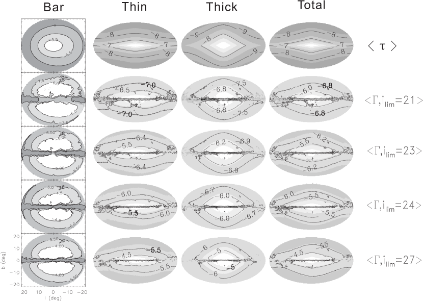
Figure 4: Distributions of the microlensing optical depths (top row) and event rates (bottom four rows). From left to right, the panels in each column represent maps of the bar component, the thin and thick disc components and the total contribution from all bar and disc components. Contours in the top row correspond to the log of the optical depth, while contours in the bottom four rows correspond to the log of events per year per square degree for the limiting source magnitudes shown on the right.

3.3 Lens mass determination

It is important to investigate the characteristics of the lens population, particularly with respect to potential follow-up work on the lenses.

In Section 2.2 we described our simplistic implementation of stellar evolution. From equation (4) it is trivial to obtain the relative contribution of the different lens populations. This is summarised in Table 2. We see that by far the majority of lenses are main-sequence stars ($\sim 80$ per cent), although a significant fraction are white/brown dwarfs. Around 1 per cent of events will be caused by neutron stars, which raises the remote, yet interesting, possibility of quasar lensing from pulsars. As has been highlighted by previous authors (e.g. Dai, Xu & Esamdin, 2010), pulsar microlensing is of great interest because for these events it may be possible to determine both the distance and transverse velocity through radio observations (and hence, via equation 1, a model independent mass determination).

However, the most promising avenue for carrying out model-independent mass determinations is for main-sequence stars. This is important because microlensing is the only method which can be applied to single stars (as opposed to all other methods of mass determination which are applicable only to stars in binary systems). As has been stated in the Introduction, to break the microlensing mass degeneracy requires a measurement of both the distance to the lens and its transverse velocity. However, to measure these lens properties requires the lens to be both bright and nearby. We investigate this by plotting maps of the event rate for various lens properties in Figs. 5 to 8.

In the near future instruments such as the ESO Gaia mission (Perryman et al., 2001) will measure parallaxes and proper motions to unprecedented accuracy for many millions of relatively bright stars. Its accuracy degrades rapidly for fainter stars, reaching accuracies of around 0.1-0.2 mas for stars at the magnitude limit of around $G=20$ mag (Bailer-Jones, 2009). This corresponds to a parallax (and hence distance) error of around 20 per cent at a distance of 2 kpc. Unfortunately, as can be seen in Fig. 5, we predict that very few lenses will be brighter than 20th magnitude in $i$-band. In Fig. 6 we have plotted the map of event rate as a function of lens brightness and distance. From this we can estimate the total event rate for lenses bright enough and near enough to be within reach of Gaia. Equation (1) shows that the error on the lens mass will be entirely dominated by the uncertainty in the parallax; if we scale the Gaia errors linearly from the bright end to the faint end (i.e. from 0.01 mas at $G=15$ mag to 0.1 mas at $G=20$ mag) and consider events for which we will be able to obtain a parallax error of 20 per cent, we find that we will obtain around 1 event every two years over the whole sky for quasars down to $i=24$. If we allow for weakly magnified events (as above), this means that LSST will be able to detect around one event per year for which we will be able to robustly determine the distance (and hence lens mass) to within 20 per cent accuracy using a parallax measurement from Gaia.

Another potential source of accurate parallax measurements is the proposed SIM-lite space mission (Unwin et al., 2008), which, if it proceeds, will enable significantly better mass determinations. With an astrometric accuracy of 0.01 mas down to $V=20$ mag, this will be able to follow-up a similar number of events to Gaia but with a ten-fold improvement in the accuracy. Even though the precision of the mass recovery will be greatly improved, the total number of events will not increase dramatically for SIM-lite since the limiting magnitude will be similar to Gaia; the only advantage to the event rate is the fact that the increased accuracy means it will be able to detect parallaxes for more distant lenses, which results in a doubling of the event rate compared to Gaia (i.e. around 2 events per year for LSST using $i=24$ quasars).

Even if we are unable to obtain accurate trigonometric parallax measurements, it will still be possible to accurately determine the proper motion for a significant number of lenses using ground-based astrometry. For example, LSST will be able to carry out astrometry at around 3 mas for $r=24$ mag. As can be seen from the lens luminosity function (Fig. 5) this covers a significantly larger number of events, many of which will have measurable proper motion (see Fig. 7). This would almost entirely break the lens mass degeneracy, but to obtain a unique mass measurement requires additional information, for example the distance (from photometric/spectroscopic techniques) or through higher-order microlensing effects. One potential higher-order effect is microlensing parallax (Gould, 1992), where the motion of the Earth as it orbits the Sun induces perturbations on the standard microlensing signal. Simulations of parallax frequency show that for distant sources the rate of parallax events towards the Galactic bulge can reach around 10 per cent (e.g. fig. 7 of Smith et al., 2005). This fraction will probably increase for lines-of-sight away from the bulge, since the velocity dispersion of disc stars is smaller than bulge stars and hence the event time-scale will increase (and hence the parallax fraction will also increase as this is related to time-scale; e.g. see fig. 6 of Smith et al., 2005). As is shown in Fig. 3, we find that 10 per cent of all events are predicted to have time-scales greater than three months.

Lens Type	Event Fraction
	(per cent)
Brown dwarf	7.5
Main sequence	78.4
White dwarf	13.1
Neutron star	0.8
Black hole	0.2

Table 2: The fraction of different lenses by population, following our simplistic implementation of stellar evolution (see Section 2.2). These fractions are obtained trivially via the IMF (equation 4).

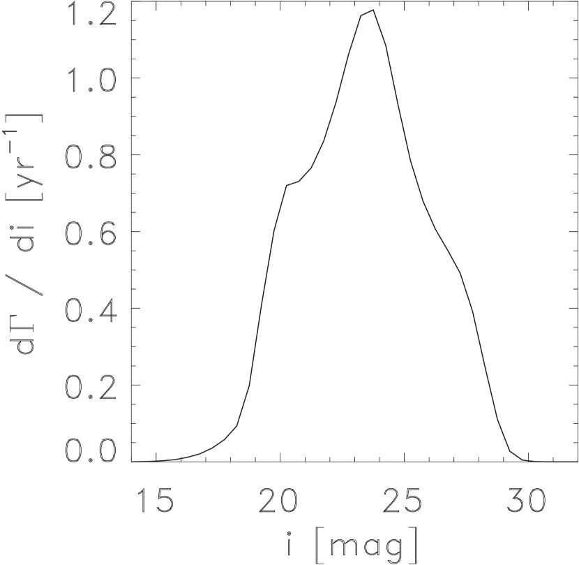
Figure 5: The distribution of $i$-band lens magnitudes, after taking into account extinction. Note that this corresponds only to the events caused by main-sequence lenses, i.e. a further 22 per cent of events have non-main-sequence lenses which we classify as ‘dark’ (see Table 2).

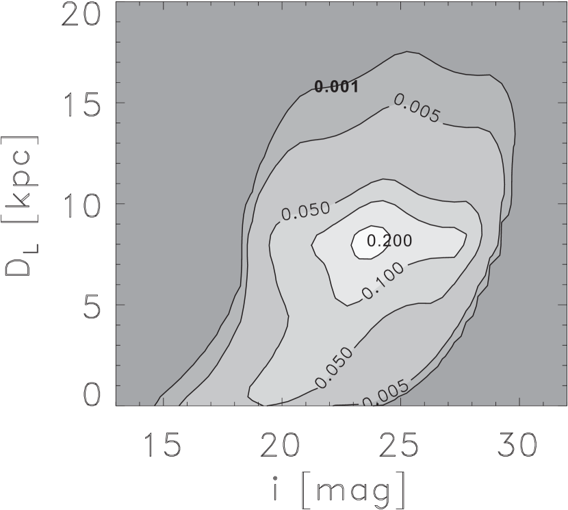
Figure 6: The all-sky event-rate map for luminous lenses as a function of lens distance and magnitude (after incorporating extinction). Contours correspond to events per year per magnitude per kpc for a limiting source magnitude of $i=24$. Note that this corresponds only to the events caused by main-sequence lenses, i.e. a further 22 per cent of events have non-main-sequence lenses which we classify as ‘dark’ (see Table 2).

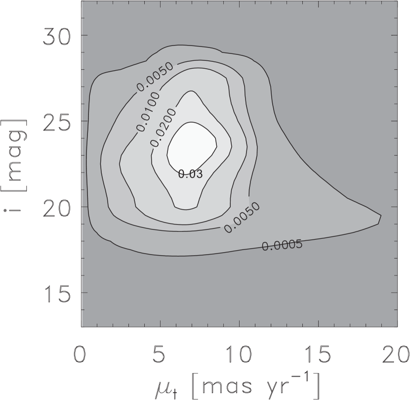
Figure 7: Similar to Fig. 6, but for lens magnitude and proper motion.

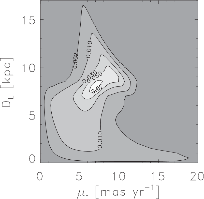
Figure 8: Similar to Fig. 6, but for lens distance and proper motion. Note that unlike Figs. 6 and 7, this plot also includes the non-main-sequence lenses (see Table 2).

4 Conclusion and discussion

In this paper we have carried out Monte Carlo simulations to make predictions for the microlensing of quasars by stars (and stellar remnants) in the Milky Way. Using a simple model of the Galaxy we have predicted the all-sky microlensing optical depth and have calculated the time-scale distributions and event rates for future large-area sky surveys, both for $i$- and $z$-band. We found that the total event rate increases rapidly with increasing magnitude limit, and predict that around 10 to 20 events will be detected per year from surveys like Pan-STARRS and LSST (see Section 3.2). Most events are caused by lenses in the thin disc, even though extinction hampers the detectability of low-latitude events. If we could identify and monitor large numbers of quasars at low latitudes (e.g. Lee et al., 2008), then it may even be possible to increase the number of detected events.

We have also highlighted how such quasar microlensing can be used to carry out robust and model-independent lens mass determinations, predicting that with accurate astrometry from Gaia or SIM-lite it will be possible to accurately recover the lens mass for around one event per year. Microlensing is uniquely placed to provide mass measurements for individual stars (as opposed to those in binary systems) and as such will undoubtedly play a crucial role in stellar astronomy.

Although these results are very promising, there are a couple of technical challenges which must be overcome in order to detect these microlensing events. In this paper we have assumed a detection efficiency of 100 per cent, which we have justified by noting that practically all events should be reasonably well-sampled by surveys like LSST. However, there are practical difficulties which will potentially reduce the efficiency.

Firstly, it is well-known that quasars themselves are intrinsically variable (e.g. Kozłowski et al., 2010). They can exhibit both long-term low-level variability as well as outburst phenomena. Indeed, one recent paper claimed to have detected a spectacular UV flare in a quasar behind M31 (Meusinger et al., 2010), although the authors admit that an alternative explanation could be microlensing. Some authors have claimed that nearly all quasars are microlensed by intervening (cosmological) compact objects (e.g. Hawkins, 1996), although more recent studies have challenged this hypothesis (e.g. de Vries et al., 2005). This latter paper analyses a variability diagnostic (the structure function) of around 40,000 quasars, concluding that the most-likely cause of quasar variability is flares due to disc instabilities. They remark that the variability is, in general, both chromatic and asymmetric. This is an important issue since the microlensing events which we are considering in this paper should be both achromatic and symmetric. Therefore one avenue for disentangling microlensing from intrinsic variability would be to utilise the multi-band photometry from surveys such as LSST. In addition, the amplitude of the quasar variability is generally at a lower level than our microlensing amplitude (e.g. Sesar et al., 2007 show that the rms scatter for quasars is $\sim 0.07$ mag in the $g$-band and, because the rms decreases for longer wavelengths, the variatbility will be even less for microlensing surveys carried out in $i$- or $z$-bands).

Although most microlensing events are symmetric and achromatic, this is not always the case. There are higher-order microlensing effects which can cause deviations from the standard symmetric and chromatic form, such as binarity in the lens or finite-source effects. Both of these will probably be of only limited importance; for standard galactic microlensing the fraction of events which show clear binary signatures is of the order 3 per cent (e.g. Skowron et al., 2008, and references therein), while for finite-source effects it is even less. Although it is safe to assume that the fraction of binary lens events for quasar sources will be similar to that for bulge sources, there is no reason to assume this will also hold for finite-source effects. If we assume that a typical quasar accretion disc is of the order $10^{13}$ cm, then the angular size will be less than a few $\mu$as. This angular size is comparable to a giant star in the Galactic bulge, which means that the finite-source effect for quasar microlensing should be no-more important than for standard Galactic microlensing; for these events finite-source effects only come into play when the amplification reaches around one hundred or more (e.g. Cassan et al., 2006). Therefore for the vast majority of quasar microlensing events the light-curves will indeed be symmetric and chromatic. For the limited number of events for which the magnification is sufficient to detect finite-source signatures, microlensing will enable constraints to be placed on the profiles of quasar accretion discs, although this could only be done in very fortuitous circumstances (e.g. when a low-redshift quasar is very highly magnified).

A second obstacle to detecting microlensing of quasars is the difficulty of identifying the quasars in the presence of a luminous lens. The quasars will be identified via cuts in colour-colour space, and so if the lens is sufficiently bright it could compromise the quasar selection. Fortunately in most cases the lenses will be significantly fainter than the sources (see Fig. 5). We calculate that for only a quarter of LSST events will the lens be brighter than the source and for just over half of all events the lenses will be fainter than the single-epoch magnitude limit of $i=24$. However, this issue will be particularly important for the events from which we wish to determine the lens mass, since for these we $require$ the lens to be luminous so that its distance and proper motion can be determined. For these events it will be important to spectroscopically confirm the presence of a quasar behind the lens, or to obtain high-resolution imaging a number of years after the event so that the lens and quasar can be resolved.

In contrast to the above challenges that hamper the detection of quasar microlensing events, there are avenues which could enhance our ability to detect events. If we could build up an accurate astrometric map of the foreground lenses and their proper motion (using, for example, data from the Gaia mission) then it could be possible to $predict$ which quasars will be lensed in advance of the amplification. This method has been suggested as an approach to detect lensing by pulsars (Dai, Xu & Esamdin, 2010) but it is equally applicable to any lens with an accurate proper motion measurment. Furthermore, this could be applied to fainter quasars, such as those provided by the complete co-added LSST survey, which will reach a depth of around $i=27$. At this magnitude the number density of quasars climbs to around 3000 per square degree (see Fig. 2.) Another avenue is that of astrometric microlensing where, instead of detecting the photometric lensing signatures, we identify the astrometric shift of the image centroid as the quasar is lensed (e.g. Høg, Novikov & Polnarev, 1995; Walker, 1995). This will be a demanding task as it requires very high precision astrometry for our faint source population; the maximum astrometric shift is 0.354 times the Einstein radius (Dominik & Sahu, 2000) and for our events typical Einstein radii are around 1 mas. As above we could envisage targeting specific quasars based on predictions from lens proper motions, but this would still require astrometry at a level of at least tens of $\mu$as.

In this work we have only considered lenses within our own Galaxy, yet one might wonder whether quasars could be lensed by stellar mass objects at cosmological distances. However, this is a remote possibility as it would require a very high density of such objects and even then the time-scales for such events are a couple of orders of magnitude longer than what we find for Galactic lenses (see, for example, Wambsganss, 2006)]. The notable exception to this, as noted in the Introduction, is the phenomena of microlensing of macro-lensed (i.e. multiple-imaged) quasars by stellar mass lenses in the intervening lensing galaxy. Here the density of lenses is sufficient to produce an optical depth of order unity and hence detecting microlensing becomes feasible. Surveys such as LSST and Pan-STARRS will have an immense impact on this field as they will monitor the light-curves for many thousands of multiply-imaged quasars.

Although we are unlikely to find events from lenses at cosmological distances (with the exception of macro-lensed quasars), it may be possible to detect lenses from populations just outside our own Galaxy. For example, one could identify quasars behind the LMC (e.g. Kozłowski & Kochanek, 2009) or M31 (Huo et al., 2010) and study their lensing by foreground stars in these galaxies. As we mentioned above, there may have already been an event of this kind detected in a quasar behind M31 (Meusinger et al., 2010).

In conclusion, we have shown that imminent ground-based surveys will be able to detect a number of quasar microlensing events every year. The efforts of Pan-STARRS and LSST will, after five years of operation, detect up to one hundred events. Although this is still too few events to constrain Galactic models due to the overwhelming numbers of parameters, it will allow for valuable consistency checks to be carried out on these models and could lead to exciting and unexpected discoveries.

References

- Alcock et al. (1993) Alcock C. et al., 1993, Nature, 365, 621
- Anguita et al. (2008) Anguita T., Faure C., Yonehara A., Wambsganss J., Kneib J.-P., Covone G., Alloin D., A&A, 2008, 481, 615
- Aubourg et al. (1993) Aubourg E. et al., 1993, Nature, 365, 623
- Bailer-Jones (2009) Bailer-Jones C.A.L., 2009, in J. Andersen, J. Bland-Hawthorn, & B. Nordström, eds, Proc. IAU Symp. 254, The Galaxy Disk in Cosmological Context, p. 210
- Bastian, Covey & Meyer (2010) Bastian N., Covey K.R., Meyer M.R., 2010, ARA&A, 48, arXiv:1001.2965
- Binney & Tremaine (1987) Binney J., Tremaine S., 1987, Galactic Dynamics (Princeton; Princeton Univ. Press)
- Binney & Tremaine (2008) Binney J., Tremaine S., 2008, Galactic Dynamics (2nd ed.; Princeton Univ. Press) (BT08)
- Bond et al. (2001) Bond I. A. et al., 2001, MNRAS, 327, 868
- Boyle et al. (2000) Boyle B. J. et al., 2000, MNRAS, 319, 1014
- Byalko (1970) Byalko A. V., 1970, Soviet Astronomy, 13, 784
- Cassan et al. (2006) Cassan A. et al., 2006, A&A, 460, 277
- Calchi Novati et al. (2005) Calchi Novati S. et al., 2005, A&A, 443, 911
- Chang & Refsdal (1979) Chang K., Refsdal S., 1979, Nature, 282, 561
- Coles et al (2009) Coles J., Saha P., Schmid H. M., 2009, arXiv:0912.0515
- Cox (1998) Cox A. N., 1999, Allen’s Astrophysical Quantities, Fourth Edition, (Springer-Verlag: New York), 489
- Croom et al. (2009) Croom S. M. et al., 2009, MNRAS, 399, 1755
- Dominik & Sahu (2000) Dominik M., Sahu, K.C., 2000, ApJ, 534, 213
- Dai, Xu & Esamdin (2010) Dai S., Xu R.X., Esamdin A., 2010, MNRAS, in press (arXiv:0912.1167)
- de Jong et al. (2006) de Jong J. T. A. et al., 2006, A&A, 446, 855
- de Jong et al. (2010) de Jong J.T.A., Yanny B., Rix H.-W., Dolphin A.E., Martin N.F., Beers T.C., ApJ, 714, 663
- de Vries et al. (2005) de Vries W.H., Becker R.H., White R.L., Loomis C., 2005, AJ, 129, 615
- Einstein (1936) Einstein A., 1936, Sci, 84, 506
- Fontanot et al. (2007) Fontanot F. et al., 2007, A&A, 461, 39
- Fukui et al. (2007) Fukui A. et al., 2007, ApJ, 670, 423
- Gaudi et al. (2008) Gaudi B. S. et al., 2008, ApJ, 677, 1268
- Górski et al. (2005) Górski K. M. et al., 2005, ApJ, 622, 759
- Gould (1992) Gould A., 1992, ApJ, 392, 442
- Gould (2000) Gould A., 2000, ApJ, 535, 928
- Griest (1991) Griest K., 1991, ApJ, 366, 412
- Gwinn et al. (1997) Gwinn C. R. et al., 1997, ApJ, 485, 87
- Hamadache et al. (2006) Hamadache C. et al., 2006, A&A, 454, 185
- Han (2008) Han C., 2008, ApJ, 681, 806
- Han & Gould (1995) Han C., Gould A., 1995, ApJ, 447, 53
- Hawkins (1996) Hawkins M.R.S., 1996, MNRAS, 278 787
- Hennawi et al. (2007) Hennawi J. F., Dalal N., Bode P., 2007, ApJ, 654, 93
- Høg, Novikov & Polnarev (1995) Høg E., Novikov I.D., Polnarev A.G., 1995, A&A, 294, 287
- Huo et al. (2010) Huo Z.-Y. et al., 2010, RAA, 10, 612
- Irwin et al. (1989) Irwin M. J. et al., 1989, AJ, 98, 1989
- Ivezić et al. (2008) Ivezić Ž., Tyson J. A., Allsman R., Andrew J., Angel R., 2008, arXiv:0805.2366
- Jordi et al (2006) Jordi K., Grebel E. K., Ammon K., 2006, A&A, 460, 339
- Kaiser et al. (2002) Kaiser N. et al., 2002, SPIE, 4836, 154
- Kayser, Refsdal & Stabell (1986) Kayser R., Refsdal S., Stabell R., 1986, A&A, 166, 36
- Kiraga & Paczyński (1994) Kiraga M., Paczyński B., 1994, ApJ, 430, L101
- Kozłowski & Kochanek (2009) Kozłowski S., Kochanek C. S., 2009, ApJ, 701, 508
- Kozłowski et al. (2010) Kozłowski S. et al., 2010, ApJ, 708, 927
- Kroupa (2002) Kroupa P., 2002, Sci, 295, 82
- Lee et al. (2008) Lee I. et al., 2008, ApJS, 175, 116
- Li et al. (2007) Li G. L. et al., 2007, MNRAS, 378, 469
- Liebes (1964) Liebes S., 1964, Phys. Rev., 133, 835
- Mao (2008) Mao S., 2008, arXiv:0811.0441
- Meusinger et al. (2010) Meusinger H., 2010, A&A, 512, 1
- Paczyński (1986) Paczyński B., 1986, ApJ, 304, 1
- Paczyński (1991, 1996) Paczyński B., 1991, ApJ, 371, L63
- Paczyński (1995) Paczyński B., 1995, Acta Astronomica, 45, 345
- Paczyński (1996) Paczyński B., 1996, ARA&A, 34, 419
- Palanque-Delabrouille et al. (1998) Palanque-Delabrouille N. et al., 1998, A&A, 332, 1
- Paulin-Henriksson et al. (2002) Paulin-Henriksson S. et al., 2002, ApJ, 576, L121
- Perryman et al. (2001) Perryman M.A.C. et al., 2001, A&A, 369, 339
- Popowski et al. (2005) Popowski P. et al., 2005, ApJ, 631, 879
- Refsdal (1964) Refsdal S., 1964, MNRAS, 128, 295
- Renn, Sauer & Stachel (1997) Renn J., Sauer T., Stachel J., 1997, Sci, 275, 184
- Richards et al. (2006) Richards G. et al., 2006, AJ, 131, 2766
- Richards et al. (2009) Richards G. et al., 2009, ApJ, 180, 67
- Sesar et al. (2007) Sesar B. et al., 2007, AJ, 134, 2236
- Schlegel et al. (1998) Schlegel D., Finkbeiner D. P., and Davis M., 1998, ApJ, 500, 525 (SFD)
- Schönrich, Binney & Dehnen (2010) Schönrich R., Binney J., Dehnen W., MNRAS, in press (arXiv:0912.3693)
- Skowron et al. (2008) Skowron J. et al., 2008, Acta Astron., 57, 281
- Smith et al. (2005) Smith M. C., Belokurov V., Evans N.W., Mao S., An J.H., 2005, MNRAS, 361, 128
- Sumi et al. (2006) Sumi T. et al., 2006, ApJ, 636, 240
- Smith et al. (2007) Smith M. C. et al., 2007, MNRAS, 379, 755
- Tisserand et al. (2007) Tisserand P. et al., 2007, A&A, 469, 387
- Thomas et al. (2005) Thomas C. L. et al., 2005, ApJ, 631, 906
- Tyson (2002) Tyson J.A., 2002, SPIE, 4836, 10
- Udalski et al. (1992) Udalski A. et al., 1992, Acta Astron., 42, 253
- Udalski et al. (2000) Udalski A. et al., 2000, Acta Astron., 50, 1
- Unwin et al. (2008) Unwin S.C. et al., 2008, PASP, 120, 38
- Uglesich et al. (2004) Uglesich R. R., 2004, ApJ, 612, 877
- Walker (1995) Walker M.A., 1995, ApJ, 453, 37
- Wambsganss (2006) Wambsganss J., 2006, in G. Meylan, P. Jetzer, P. North, P. Schneider, C. S. Kochanek, & J. Wambsganss, eds, Saas-Fee Advanced Course 33: Gravitational Lensing: Strong, Weak and Micro
- Wood & Mao (2005) Wood A., Mao S., 2005, MNRAS, 362, 945
- Wyrzykowski et al. (2009) Wyrzykowski Ł. et al., 2009, MNRAS, 397, 1228
- Wyrzykowski et al. (2010) Wyrzykowski Ł. et al., 2010, MNRAS, in press (arXiv:1004.5247)