Free fall and self-force: an historical perspective

Abstract

Free fall has signed the greatest markings in the history of physics through the leaning Pisa tower, the Cambridge apple tree and the Einstein lift. The perspectives offered by the capture of stars by supermassive black holes are to be cherished, because the study of the motion of falling stars will constitute a giant step forward in the understanding of gravitation in the regime of strong field. After an account on the perception of free fall in ancient times and on the behaviour of a gravitating mass in Newtonian physics, this chapter deals with last century debate on the repulsion for a Schwarzschild black hole and mentions the issue of an infalling particle velocity at the horizon. Further, black hole perturbations and numerical methods are presented, paving the way to the introduction of the self-force and other back-action related methods. The impact of the perturbations on the motion of the falling particle is computed via the tail, the back-scattered part of the perturbations, or via a radiative Green function. In the former approach, the self-force acts upon the background geodesic; in the latter, the geodesic is conceived in the total (background plus perturbations) field. Regularisation techniques (mode-sum and Riemann-Hurwitz $z$ function) intervene to cancel divergencies coming from the infinitesimal size of the particle. An account is given on the state of the art, including the last results obtained in this most classical problem, together with a perspective encompassing future space gravitational wave interferometry and head-on particle physics experiments. As free fall is patently non-adiabatic, it requires the most sophisticated techniques for studying the evolution of the motion. In this scenario, the potential of the self-consistent approach, by means of which the background geodesic is continuously corrected by the self-force contribution, is examined.

1 Introduction

The two-body problem in general relativity remains one of the most interesting problems, being still partially unsolved. Specifically, the free fall, one of the eldest and classical problems in physics, has characterised the thinking of the most genial developments and it is taken as reference to measure our progress in the knowledge of gravitation. Free fall contains some of the most fundamental questions on relativistic motion. The mathematical simplification, given by the reduction to a 2-dimensional case, and the non-likelihood of an astrophysical head-on collision should not throw a shadow on the merits of this problem. Instead, it may be seen as an arena where to explore part of the relevant features that occur to general orbits, e.g. the coupling between radial and time coordinates.

Although it is easily argued that radiation reaction has a modest impact on radial fall due to the feebleness of cumulative effects (anyhow, in case of high or even relativistic - a fraction of $c$ - initial velocity of the falling particle, it is reasonable to suppose a non-modest impact on the waveform and possibly the existence of a signature), it would be presumptuous to consider free fall simpler than circular orbits, or even elliptic orbits if in the latter adiabaticity may be evoked. Adiabaticity has been variously defined in the literature, but on the common ground of the secular effects of radiation reaction occurring on a longer time scale than the orbital period. One definition refers to the particle moving anyhow, although radiating, on the background geodesic (local small deviations approximation), of obviously no-interest herein; another, currently debated for bound orbits, to the secular changes in the orbital motion being stemmed solely by the dissipative effects (radiative approximation); the third to the radiation reaction time scale being much longer than the orbital period (secular approximation), which is a rephrasing of the basic assumption.

But in radial fall such an orbital period doesn’t exist. And as the particle falls in, the problem becomes more and more complex. In curved spacetime, at any time the emitted radiation may backscatter off the spacetime curvature, and interact back with the particle later on. Therefore, the instantaneous conservation of energy is not applicable and the momentary self-force acting on the particle depends on the particle’s entire history. There is an escape route, though, for periodic motion. But energy-momentum balance can’t be evoked in radial fall, lacking the opportunity of any adiabatic averaging. The particle reaction to its radiation has thus to be computed and implemented immediately to determine the effects on the subsequent motion. It is a no-compromise analysis, without shortcuts. Thus, the computation and the application of the back-action all along the trajectory and the continuous correction of the background geodesic, it is the only semi-analytic way to determine motion in non-adiabatic cases. And once this self-consistent approach shall be mastered for radial infall, where simplification occurs for the two-dimensional nature of the problem, it shall be applicable to generic orbits.

It is worth reminding that the non-adiabatic gravitational waveforms are one of the original aims of the self-force community, since they express i) the physics closer to the black hole horizon; ii) the most complex trajectories; iii) the most tantalising theoretical questions.

The head-on collisions of black holes and the associated radiation reaction were evoked recently in the context of particle accelerators and thereby showing the richness of the applicability of the radial trajectory also beyond the astrophysical realm. As gravity is claimed by some authors to be the dominant force in the transplanckian region, the use of general relativity is adopted for their analysis.

This chapter reviews the problem of free fall of a small mass into a large one, from the beginning of science, whatever this may mean, to the application of the self-force and of a concurring approach, in the last fourteen years. There is no pretension of exhaustiveness and, furthermore, justifiably or not, from this review some topics have been disregarded, namely: any orbit different from radial fall; radiation reaction in electromagnetism; but also the head-on of comparable masses and Kerr geometry, post-Newtonian (pN) and effective one-body (EOB) methods; quantum corrections to motion.

Herein, the terms of self-force and radiation reaction are used rather loosely, though the latter does not include non-radiative modes. Thus, the self-force describes any of the effects upon an object’s motion which are proportional to its own mass. Nevertheless, to the term self-force is often associated a specific method and it is preferable to adopt the term back-action whenever such association is not meant.

Geometric units ($G=c=1$) and the convention (-,+,+,+) are adopted, unless otherwise stated. The full metric is given by ${\bar{g}}_{\alpha\beta}(t,r)=g_{\alpha\beta}(r)+h_{\alpha\beta}(t,r)$ where $g_{\alpha\beta}$ is the background metric of a black hole of mass $M$ and $h_{\alpha\beta}$ is the perturbation caused by a test particle of mass $m$.

2 The historical heritage

The analysis of the problem of motion certainly did not start with a refereed publication and it is arduous to identify individual contributions. Therefore, an arbitrary and convenient choice has led to select only renowned names.

Aristotélēs in the fourth century B.C. analysed motion qualitatively rather than quantitatively, but he was certainly more geared to a physical language than his predecessors. His views are scattered through his works, though mainly exposed in the Corpus Aristotelicum, collection of the works of Aristotélēs, that has survived from antiquity through Medieval manuscript transmission ar . He held that there are two kinds of motion for inanimate matter, natural and unnatural. Unnatural motion is when something is being pushed: in this case the speed of motion is proportional to the force of the push. Natural motion is when something is seeking its natural place in the universe, such as a stone falling, or fire rising. For the natural motion of objects falling to Earth, Aristotélēs asserted that the speed of fall is proportional to the weight, and inversely proportional to the density of the medium the body is falling through. He added, though, that there is some acceleration as the body approaches more closely its own element; the body increases its weight and speeds up. The more tenuous a medium is, the faster the motion. If an object is moving in void, Aristotélēs believed that it would be moving infinitely fast.

After two centuries, Hipparkhos said, through Simplikios si , that bodies falling from high do experience a restraining factor which accounts for the slower movement at the start of the fall.

Gravitation was a domain of concern in the flourishing Islamic world between the ninth and the thirteenth century by ibn Shākir, al-Bīrūnī, al-Haytham, al-Khazini. It is doubtful whether gravitation was in their minds in the form of a mutual attraction of all existing bodies, but the debate acquired significant depth, although not benefiting of any experimental input. Conversely, in Islamic countries experiments were performed as deemed necessary for the development of science. In this sense, there was a large paradigmic shift with respect to Greek philosophers, more oriented to abstract speculations.

Leonardo da Vinci stated that each object doesn’t move by its own, and when it moves, it moves under an unequal weight (for a higher cause); and when the wish of the first engine stops, immediately the second stops lv . Further, in the context of 15^th century gravitation, da Vinci compared planets to magnets for their mutual attraction.

Perception of the beginning of modern science in the early seventeenth century is connected on one hand to a popular legend, according to which Galilei dropped balls of various densities from the Tower of Pisa, and found that lighter and heavier ones fell at the same speed (in fact, he did quantitative experiments with balls rolling down an inclined plane, a form of falling that is slow enough to be measured without advanced instruments); on the other hand, modern science developed when the natural philosophers abandoned the search for a cause of the motion, in favour of the search for a law describing such motion. The law of fall, stating that distances from rest are as the squares of the elapsed times, appeared already in 1604 ga1604 and further developed in two famous essays ga1632 ; ga1638 .

After another century, another legend is connected to Newton wh97 who indeed himself told that he was inspired to formulate his theory of gravitation ne1687 by watching the fall of an apple from a tree as reported by W. Stuckeley and J. Conduit. The fatherhood of the inverse square law, though, was claimed by R. Hooke and it can be traced back even further in the history of physics.

The pre-Galilean physics, see Drake dr00 , had an insight on phenomena that is not to be dismissed at once. For instance, the widespread belief that fall is unaffected by the mass of the falling object shall be examined throughout the chapter, through the concept of Newtonian back-action and through the general relativistic analysis of the capture of stars by supermassive black holes.

3 Uniqueness of acceleration and the Newtonian back-action

One of the most mysterious and sacred laws in general relativity is the equivalence principle (EP). Confronted with “the happiest thought” of Einstein’s life, it is a relief for those who adventure into its questioning to find out that notable relativists share this humble opinion. This principle is variously defined and here below some most popular versions are listed:

1. All bodies equally accelerate under inertial or gravitational forces.

2. All bodies equally accelerate independently from their internal composition.

   In general relativity, the language style gets more sophisticated:

3. At every spacetime point of an arbitrary gravitational field, it is possible to choose a locally inertial coordinate system such that the laws of nature take the same form as in an unaccelerated coordinate system. The laws of nature concerned might be all laws (strong EP), or solely those dealing with inertial motion (weak EP) or all laws but those dealing with inertial motion (semi-strong EP).

4. A freely moving particle follows a geodesic of spacetime.

It is evident that both conceptually and experimentally, the above different statements are not necessarily equivalent, although they can be connected to each other (for instance: the EP states that the ratio of gravitational mass to inertial mass is identical for all bodies and convenience suggests that this ratio is posed equal to unity). In this chaper, only the fourth definition will be dealt with and interestingly, it can be reformulated, see Detweiler and Whiting dewh03 ; whde03 , in terms of geodesic motion in the perturbed field. Then, the back-action results into the geodesic motion of the particle in the metric $g_{\alpha\beta}(r)+h_{\alpha\beta}^{R}(t,r)$ where $h_{\alpha\beta}^{R}$ is the regular part of the perturbation caused by a test particle of mass $m$. Thus, the concept of geodesic motion is adapted to include the influence of $m$ through $h_{\alpha\beta}^{R}$.

A teasing paradox concerning radiation has been conceived relative to a charge located in an Earth orbiting spacecraft. Circularly moving charges do radiate, but relative to the freely falling space cabin the charge is at rest and thus not radiating. Ehlers ri06 solves the paradox by proposing that “It is necessary to restrict the class of experiments covered by the EP to those that are isolated from bodies of fields outside the cabin”. The transfer of this paradox to the gravitational case, including the case of radial fall, is immediate.

The EP is receptive of another criticism directed at the relation between the foundations of relativity and their implementation: it is somehow confined to the introduction of general relativity, while, for the development of the theory, a student of general relativity may be rather unaware of it.

A popular but wrong interpretation of the EP states that all bodies fall with the same acceleration independently from the value of their mass (sometimes referred as the uniqueness of acceleration). This view is portrayed or vaguely referred to in some undergraduate textbooks, and anyhow largely present in various websites. Concerning the uniqueness of acceleration, non-radiative relativistic modes in a circular orbit were analysed by Detweiler and Poisson depo04 , who showed how the low multipole contributions to the gravitational self-acceleration may produce physical effects, within gauge arbitrariness ($l=0$ determines a mass shift, $l=1$ a centre of mass shift). In depo04 , the stage is set by a discussion on the gravitational self-force in Newtonian theory for a circular orbit. Herein, exactly the same pedagogical demonstration of theirs is applied to free fall.

A small particle of mass $m$ is in the gravitational field of a much larger mass $M$. The origin of the coordinate system coincides with the centre of mass. The positions of $M$, $m$ and a field point $P$ are given by $\overrightarrow{\rho}$, $\overrightarrow{R}$ and $\overrightarrow{r}$, respectively (the absolute value of $\overrightarrow{r}$ is $r$ and $m\overrightarrow{R}+M\overrightarrow{\rho}=0$). In case of the sole presence of $M$, the potential and the acceleration at $P$ are given by:

$$\Phi_{0}(r)=-\frac{M}{r},~{}~{}~{}~{}~{}~{}~{}~{}~{}~{}~{}~{}~{}~{}~{}~{}~{}~{}~{}~{}\overrightarrow{g}_{0}(r)=-\nabla\Phi_{0}(r)=-\frac{M}{r^{3}}\overrightarrow{r}.$$ (1)

If $m$ is also present, $M$ is displaced from the origin and the potential is:

$$\Phi(r)=-\frac{M}{|\overrightarrow{r}-\overrightarrow{\rho}|}-\frac{m}{|\overrightarrow{r}-\overrightarrow{R}|}.$$ (2)

Since $m\ll M$, eq. (2) is rewritten in the form of a small variation, that is $\Phi(r)=\Phi_{0}(r)+\delta\Phi(r)$ or else $\delta\Phi(r)=\Phi(r)-\Phi_{0}(r)$; thus:

$$\delta\Phi(r)=\underbrace{-\frac{m}{|\overrightarrow{r}-\overrightarrow{R}|}}_{\Phi_{S}}~{}\underbrace{-\frac{M}{|\overrightarrow{r}-\overrightarrow{\rho}|}+\frac{M}{r}}_{\Phi_{R}}.$$ (3)

The potential $\delta\Phi(r)$ determines a field that exerts a force on $m$, that is the back-action of the particle. The singular term $\Phi_{S}$ diverges, but isotropically around the particle position and thus not contributing to the particle motion. Instead, the remaining regular part acts on the particle. Since $m\ll M$, the regular parts of the potential and of the acceleration, being $\nabla={\partial_{r}}(\overrightarrow{r}/{r})$, are:

$$\Phi_{R}(r)\simeq-\frac{M}{r}\left[1-\frac{m}{M}\frac{\overrightarrow{R}\cdot\overrightarrow{r}}{r^{2}}\right]+\frac{M}{r}=m\frac{\overrightarrow{R}\cdot\overrightarrow{r}}{r^{3}},$$ (4)

$$\overrightarrow{g}_{R}(r)=-\nabla\Phi_{R}(r)=m\frac{3(\overrightarrow{R}\cdot\overrightarrow{r})\overrightarrow{r}-r^{2}\overrightarrow{R}}{r^{5}}.$$ (5)

At the particle position, the two components of the acceleration are:

$$\overrightarrow{g}_{R}(R)=2m\frac{\overrightarrow{R}}{R^{3}},~{}~{}~{}~{}~{}~{}~{}~{}~{}~{}~{}~{}~{}~{}~{}~{}~{}~{}~{}~{}~{}~{}\overrightarrow{g}_{0}(R)=-M\frac{\overrightarrow{R}}{R^{3}},$$ (6)

and finally the total acceleration is given by (in vector and scalar form):

$$\overrightarrow{g}(R)=\overrightarrow{g}_{0}(R)+\overrightarrow{g}_{R}(R)=-\frac{M-2m}{R^{3}}\overrightarrow{R},$$ (7)

$${g}(R)=-\frac{M}{R^{2}}\left(1-2\frac{m}{M}\right).$$ (8)

The Newtonian back-action of a particle of mass $m$ falling into a much larger mass $M$ is expressed as a correction to the classical value. This result is more easily derived, if the partition between singular and regular parts and the vectorial notation is left aside. The force exerted on $m$ is (the origin of coordinate system is made coincident with the centre of mass for simplicity, so that $mR=M\rho$):

$$m{\ddot{R}}=-\frac{Mm}{(\rho+R)^{2}},$$ (9)

and thus

$${\ddot{R}}=-\frac{M}{R^{2}\left(1+\displaystyle\frac{\rho}{R}\right)^{2}}\simeq-\frac{M}{R^{2}}\left(1-2\frac{m}{M}\right),$$ (10)

and

$${\ddot{R}}=-\frac{M}{R(\rho+R)\left(1+\displaystyle\frac{\rho}{R}\right)}\simeq-\frac{M}{R(\rho+R)}\left(1-\frac{m}{M}\right).$$ (11)

It appears from the preceding computations that the falling mass is slowed down by a factor (1 or 2) proportional to its own mass and dependent upon the measurement approach adopted. It may be argued that the $m/M$ term arises because the computation is referred to the centre of mass, but to shift the centre of mass to the centre of $M$ is equivalent to deny the influence of $m$.

But instead, what about the popular belief that heavier objects fall faster? Let us consider the mass $m$ at height $h$ from the soil and the Earth radius $R_{\oplus}$; since $\rho+R=h+R_{\oplus}$, it is found that:

$${\ddot{h}}=-\frac{M}{\left(h+R_{\oplus}\right)^{2}}\left(1+\frac{m}{M}\right).$$ (12)

The mass is now falling faster thanks to a different observer system and the popular belief appears being confirmed. On the other hand, in a coordinate system whose origin is coincident and comoving with the centre of mass of the larger body $M$, any back-action effect disappears. For $d$, the distance between the two bodies, it is well known that:

$$m{\ddot{d}}=\frac{mM}{d^{2}}.$$ (13)

Nevertheless, the translational speed of the moving centre of mass of $M$ (if the latter is fixed, any influence of $m$ is automatically ruled out) is depending upon the value of $m$ and the same applies to eq. (9): it is not possible to find an universal reference frame in which the centre of mass moves equally for all various falling masses. Thus, the uniqueness of acceleration is result of an approximation, although often portrayed as an exact statement, or else consequence of gauge choice. The uniqueness of acceleration holds as long as the values of the masses of the falling bodies are negligible. Correctly stated, the principle hardly sounds like a principle: all bodies fall with the same acceleration independently from their mass, if … we neglect their mass. Although the preceding is elementary, misconceptions tend to persist in colleges and higher education.

It is concluded that the Newtonian back-action manifests itself with different numerical factors possibly carrying opposite sign (from the Pisa tower - 100 pisan arms tall - for an observer situated at its feet, Newtonian back-action shows roughly as proportional to $1.7\times 10^{-24}~{}m/s^{2}$ for each falling kilogram). This feature corresponds to the gauge freedom in general relativity.

For the latter, when considering perturbations, the energy radiated through gravitational waves is proportional to $m^{2}/M$ and thus the energy leaking from the nominal motion. Therefore, the concept of uniqueness of acceleration is further affected, as it will be shown further.

Finally, it is quoted dewh03 that with only local measurements, the observer has no means of distinguishing the perturbations from the background metric. In the next section, it is shown that the concept of locality or non-locality of measurements associated to free fall, even without taking into account radiation reaction, is far from being evident and has fueled a controversy for more than $90$ years.

4 The controversy on the repulsion and on the particle velocity at the horizon

The concept of light being trapped in a star was presented in 1783 by Michell mi1784 in front of the Royal Society audience and later by Laplace la1796 ; la1799 . Preti pr09 describes the close resemblance between the algebraic formulation of Laplace la1799 and the concept of a black hole, term coined in 1967 by Wheeler wh67 . In the last century, the Earth, once the attracting mass of reference, was silently replaced by the black hole. But, as many centuries before and after Newtonian gravity were necessary to formulate motion on the Earth, it should not be a surprise that it is taking more than a century to resolve the same Newtonian questions in the more complex Einsteinian general relativity on a black hole.

The existence and the detectability of gravitational waves, the validity of the quadrupole formula are among the notorious debates that have characterised general relativity, as described by Kennefick ke07 . But closer to the topic of this chapter is the, surprisingly since almost endless, controversy on the radial motion in the unperturbed Schwarzschild or properly Schwarzschild-Droste (henceforth SD) metric sc16 ; dr16a ; dr16b , intertwined with the early debates on the apparent singularity at $2M$ and on the belief of the impenetrability of this singularity due to the infinite value of pression at $9/4~{}M$.

Most references for analysis of orbital motion, e.g. the first comprehensive analysis by Hagihara ha31 or the later and popular book by Chandrasekhar ch83 , don’t address this debate, that has invested names of the first rank in the specialised early literature.

An historically oriented essay by Eisenstaedt ei87 critically scrutinises the relation that relativists have with free fall. This section does not have any pretension of topical (e.g. photons in free fall are not dealt with) or bibliographical completeness. The questions posed in this debate concern the radial fall of a particle into a SD black hole and may be summarised as:

• Is there an effect of repulsion such that masses are bounced back from the black hole? Or more mildly, does the particle speed, although always inward, reaches a maximal value and then slows down? And if so, at which speed or at which coordinate radius?

• Does the particle reaches the speed of light at the horizon?

The discussion is largely a reflection of coordinate arbitrariness (and unawareness of its consequences), but the debaters showed sometimes a passionate affection to a coordinate frame they considered more suitable for a ‘real physical’ measurement than other gauges. Further, ill-defined initial conditions at infinity, inaccurate wording (approaching rather than equalling the speed of light), sometimes tortuous reasonings despite the great mathematical simplicity, scarce propension to bibliographic research with consequent claim of historical findings loma09 , they all contributed to the duration of this debate. The approach of this section is to cut through any tortuous reasoning pd08 and show the essence of the debate by means of a clean and simple presentation, thereby paying the price of oversimplification.

Four types of measurements can be envisaged: local measurement of time $dT$, non-local measurement of time $dt$, local measurement of length $dR$, non-local measurement of length $dr$. Locality is somewhat a loose definition, but it hints at those measurements by rules and clocks affected by gravity (of the SD black hole) and noted by capital letters $T,R$, while non-locality hints at measurements by rules and clocks not affected by gravity (of the SD black hole) and noted by small letters $t,r$. Therefore, for determining (velocities and) accelerations, four possible combinations do exist:

• Unrenormalised acceleration $d^{2}r/dt^{2}$;

• Semi-renormalised acceleration $d^{2}R/dt^{2}$;

• Renormalised acceleration $d^{2}R/dT^{2}$;

• Semi-renormalised acceleration $d^{2}r/dT^{2}$.

The latter hasn’t been proposed in the literature and discussion will be limited to the first three types. The former two present repulsion at different conditions, while the third one never presents repulsion.

The first to introduce the idea of gravitational repulsion was Droste dr16a ; dr16b himself. He defines:

$$dR=\frac{dr}{\sqrt{1-\displaystyle\frac{2M}{r}}},$$ (14)

which, after integration, Droste called the distance $\delta$ from the horizon. This quantity is derived from the SD metric posing $dt=0$, delicate operation since the relation between proper and coordinate times varies in space as explained by Landau and Lifshits lali41 ; thus it may be accepted only for a static observer (obviously the notion of static observer raises in itself a series of questions, see e.g. Doughty do81 , Taylor and Wheeler tawh00 .). Through a Lagrangian and the relation of eq. (14), for radial trajectories Droste derives that the semi-renormalised velocity and acceleration are given by ($A$ is a constant of motion, equal to unity for a particle falling with zero velocity at infinity):

$$\frac{dR}{dt}=-\sqrt{\left(1-\frac{2M}{r}\right)\left(1-A+\frac{2AM}{r}\right)},$$ (15)

$$\frac{d^{2}R}{dt^{2}}=-\frac{M}{r^{2}}\left[\sqrt{1-\frac{2M}{r}}-{\displaystyle\frac{2\left(\displaystyle dR/dt\right)^{2}}{\sqrt{1-\displaystyle\frac{2M}{r}}}}\right]=\frac{M}{r^{2}}\left(1-2A+\frac{4AM}{r}\right)\sqrt{1-\frac{2M}{r}},$$ (16)

where the constant of motion $A$ is given by:

$$A=\left(1-\frac{2M}{r}\right)^{-1}-({dr}/{dt})^{2}\left(1-\frac{2M}{r}\right)^{-3}.$$

From eq. (16), two conditions may be derived for the semi-renormalised acceleration, for either of which the repulsion (the acceleration is positive) occurs for $A=1$ if $r<4M$ or else $dR/dt>\sqrt{1/2}\sqrt{1-2M/r}$.

Instead in his thesis dr16a , Droste investigated the unrenormalised velocity acceleration and for zero velocity at infinity, they are:

$$\frac{dr}{dt}=-\left(1-\frac{2M}{r}\right)\sqrt{\frac{2M}{r}},$$ (17)

$$\frac{d^{2}r}{dt^{2}}=-\frac{M}{r^{2}}\left[1-\frac{2M}{r}-{\displaystyle\frac{3\left(\displaystyle dr/dt\right)^{2}}{1-\displaystyle\frac{2M}{r}}}\right]=-\frac{M}{r^{2}}\left(1-\frac{2M}{r}\right)\left(1-\frac{6M}{r}\right),$$ (18)

for which repulsion occurs if, still for a particle falling from infinity with zero initial velocity, $r<6M$ or else $dr/dt>1/\sqrt{3}(1-2M/r)$.

The impact of the choice of coordinates on generating repulsion was not well perceived in the early days of general relativity. Further, many notable authors as Hilbert hi17 ; hi24 , Page pa20 , Eddington ed20 , von Laue vl21 in the German original version of his book, Bauer ba22 , de Jans dj23 ; dj24a ; dj24b although indirectly by referring to the German version of vl21 , arrive independently and largely ignoring the existence of Droste’s work, to the same conclusions in semi-renormalised or unrenormalised coordinates.

The initial conditions may astray the particle from being attracted by the gravitating mass. Indeed, Droste dr16b and Page pa20 refer to particles having velocities at infinity equal or larger of $1/\sqrt{2}$ for the semi-renormalised coordinates and equal or larger of $1/\sqrt{3}$ for the unrenormalised coordinates. These conditions dictate to Droste and Page that the particle is constantly slowed down when approaching the black hole and therefore impose to gravitation an endless repulsive action.

In the later French editions of his book, von Laue vl21 writes the radial geodesic in proper time, but it is only in 1936 that Drumaux dr36 fully exploits it. Drumaux criticises the use of the semi-renormalised velocity and considers eq. (14) as defining the physical measurement of length $dR$. Similarly, the relation between coordinate and proper times (for $dr=0$) provides the physical measurement of time $dT$:

$$dT=\sqrt{1-\frac{2M}{r}}dt.$$ (19)

Thereby, Drumaux derives the renormalised velocity and acceleration in proper time:

$$\frac{dR}{dT}=\sqrt{\frac{2M}{r}},$$ (20)

$$\frac{d^{2}R}{dT^{2}}=-\frac{M}{r^{2}}\sqrt{1-\frac{2M}{r}},$$ (21)

for which no repulsion occurs. This approach is followed by von Rabe vr47 , Whittaker wh53 , Srnivasa Rao sr66 , Zel’dovich and Novikov zeno67 . Nevertheless, McVittie, almost thirty years after Drumaux mv56 , still reaffirms that the particle is pushed away by the central body as do Treder tr72 , also in cooperation with Fritze trfr75 , Markley ma73 , Arifov ar80 ; ar81 , McGruder mg82 . A discussion on radar and Doppler measurements with semi-renormalised measurements was offered by Jaffe and Shapiro jash72 ; jash73 . The controversy seems to be extinguished in the 80s, although recent research papers still refer to it, e.g. Kutschera and Zajiczek kuza09 .

For the particle’s velocity at the horizon, another, though related, debate has taken place in some of the above mentioned references as well as in Landau and Lifshits lali41 , Baierlein ba73 , Janis ja73 ; ja77 , Rindler ri79 , Shapiro and Teukolsky shte83 , Frolov and Novikov frno98 , Mitra mi00 , Crawford and Tereno crte02 , Müller mu08 the last ones being recently published. Whether the velocity is $c$ or less, it is still the question posed by these papers.

The further step forward in the analysis of a freely falling mass into a SD black hole has taken place in the period from 1957 to 1997. In these forty years, the falling mass finally radiates energy (the radiated gravitational power is proportional to the square of the third time derivative of the quadrupole moment which is different than zero), but its motion is still unaffected by the radiation emitted. The influence of the radiation on the motion of a particle of infinitesimal size wasn’t dealt with until 1997.

5 Black hole perturbations

Perturbations were first dealt with by Regge and Wheeler re57 ; rewh57 , where a SD black hole was shown to regain stability after undergoing small vibrations about its spherical form, if subjected to a small perturbation. The analysis was carried out thanks to the first application to a black hole of the Einstein equation at higher order.

The SD metric describes the background field $g_{\mu\nu}$ on which the perturbations $h_{\mu\nu}$ arise. It is given by:

$$ds^{2}=-\left(1-\frac{2M}{r}\right)dt^{2}+\left(1-\frac{2M}{r}\right)^{-1}dr^{2}+r^{2}\left(d\theta^{2}+\sin^{2}\theta d\phi^{2}\right).$$ (22)

Eq. (22) originates from the Einstein field equation in vacuum, consisting in the vanishing of the Ricci tensor $R_{\mu\nu}=0$.

Instead, the Regge-Wheeler equation derives from the vacuum condition, but this time posed on the first order variation of the Ricci tensor $\delta R_{\mu\nu}=0$. The generic form of the variation of the Ricci tensor was found by Eisenhart ei26 and it is given by: $\delta R_{\mu\nu}=-\delta\Gamma^{\beta}_{\mu\nu;\beta}+\delta\Gamma^{\beta}_{\mu\beta;\nu}$ where the tensor $\delta\Gamma^{\alpha}_{\beta\gamma}$, variation of the Christoffel symbol (a pseudo-tensor), is: $\delta\Gamma^{\alpha}_{\beta\gamma}=1/2~{}g^{\alpha\nu}(h_{\beta\nu;\gamma}+h_{\gamma\nu;\beta}-h_{\beta\gamma;\nu})$, being the perturbation $h_{\mu\nu}=\delta g_{\mu\nu}$. Replacing the latter in the vanishing variation of the Ricci tensor, a system of ten second order differential equations in $h_{\mu\nu}$ was obtained. Exploiting spherical symmetry, finally Regge and Wheeler got a vacuum wave equation out of the three odd-parity equations giving birth to a field that has grown immensely from the end of the 50s.

Zel’dovich and Novikov zeno64 first considered the problem of gravitational waves emitted by bodies moving in the field of a star, on the basis of the quadrupole formula, thus at large distances from the horizon, where only a minimal part of the radiation is emitted.

Whilst a less known semi-relativistic work by Ruffini and Wheeler ruwh71a ; ruwh71b appeared in the transition from the 60s to the 70s, it was the work by Zerilli ze70a ; ze70b ; ze70c , where the source of perturbations was considered in the form of a radially falling particle, that opened the way to study free fall in a fully, although linearised, relativistic regime at first order. The Zerilli equation rules even-parity waves in the presence of a source, i.e. a freely falling point particle, generating a perturbation for which the difference from the SD geometry is small. The energy-momentum tensor $T_{\mu\nu}$ is given by the integral of the world-line of the particle, the integrand containing a four-dimensional invariant $\delta$ Dirac distribution for representation of the point particle trajectory. The vanishing of the covariant divergence of $T_{\mu\nu}$ is guaranteed by the world-line being a geodesic in the background SD geometry; in this way, the problem of the linearised theory on flat spacetime (for which the particle moves on a geodesic of flat space which determines uniform motion and thereby without emission of radiation) is avoided. Finally, the complete description of the gravitational waves emitted is given by the symmetric tensor $h_{\mu\nu}$, function of $r$, $\theta$, $\phi$ and $t$.

The formalism can be summarised as follows ze70a ; ze70b ; ze70c . Due to the spherical symmetry of the SD field, the linearised field equations for the perturbation $h_{\mu\nu}$ are in the form of rotationally invariant operator on $h_{\mu\nu}$, set equal to the energy-momentum tensor also expressed in spherical tensorial harmonics:

$$Q[h_{\mu\nu}]\propto T_{\mu\nu}[\delta(z_{u})],$$ (23)

where the $\delta(z_{u})$ Dirac distribution represents the point particle on the unperturbed trajectory $z_{u}$.

The rotational invariance is used to separate out the angular variables in the field equations. For the spherical symmetry on the 2-dimensional manifold on which $t,r$ are constants under rotation in the $\theta,\phi$ sphere, the ten components of the perturbing symmetric tensor transform like three scalars, two vectors and one tensor:

$$h_{tt},h_{tr},h_{rr}~{}~{}~{}~{}~{}~{}~{}~{}~{}~{}~{}~{}~{}~{}~{}~{}(h_{t\theta};h_{t\phi}),(h_{r\theta};h_{r\phi})~{}~{}~{}~{}~{}~{}~{}~{}~{}~{}~{}~{}~{}~{}~{}~{}\left(\matrix{h_{\theta\theta}&h_{\theta\phi}\cr h_{\phi\theta}&h_{\phi\phi}}\right).$$

In the Regge-Wheeler-Zerilli formalism, the even perturbations (the source term for the odd perturbations vanishes for the radial trajectory and given the rotational invariance through the azimuthal angle, only the index referring to the polar or latitude angle survives), going as $(-1)^{l}$, are expressed by the following matrix:

$$h_{\mu\nu}\!\!=\!\!\!\left(\!\!\matrix{\left(1-\frac{\displaystyle 2M}{\displaystyle r}\right)H_{0}Y&\!\!\!\!\!\!\!\!\!\!\!\!\!\!H_{1}Y&\!\!\!\!\!\!\!\!\!\!\!h_{0}Y_{,\theta}&\!\!\!\!\!\!\!\!\!\!\!\!\!h_{0}Y_{,\phi}\cr sym&\!\!\!\!\!\!\!\!\!\!\!\!\!\left(1-\frac{\displaystyle 2M}{\displaystyle r}\right)^{-1}H_{2}Y&\!\!\!\!\!\!h_{1}Y_{,\theta}&\!\!\!\!\!\!\!\!\!\!\!h_{1}Y_{,\phi}\cr sym&\!\!\!\!\!\!\!\!\!\!\!\!\!\!sym&\!\!\!\!\!\!\!\!\!\!\!r^{2}\left[KY+GY_{,\theta\theta}\right]&\!\!\!\!\!\!\!\!\!\!\!r^{2}G\left(Y_{,\theta\phi}-\cot\theta Y_{,\phi}\right)\cr sym&\!\!\!\!\!\!\!\!\!\!\!\!\!\!sym&\!\!\!\!\!\!\!\!\!\!\!sym&\!\!\!\!\!\!\!\!\!\!\!r^{2}\sin^{2}\!\theta\!\!\left[K\!+\!G\!\left(\!\frac{\displaystyle Y_{,\phi\phi}}{\displaystyle\sin^{2}\!\theta}\!+\!\cot\theta Y_{,\theta}\right)\right]}\!\!\right),$$ (24)

where $H_{0},H_{1},H_{2},h_{0},h_{1},K,G$ are functions of $(t,r)$ and the $l$ multipole index isn’t displayed. After angular dependence separation, the seven functions of $(t,r)$ are reduced to four due to a gauge transformation for which $G=h_{0}=h_{1}=0$, i.e. the Regge-Wheeler gauge.

For a point particle of proper mass $m$, represented by a Dirac delta distribution, the stress-energy tensor is given by:

$$T^{\alpha\beta}=m\frac{u^{\alpha}u^{\beta}}{u^{0}r^{2}}~{}\delta[r-z_{u}(t)]\delta^{2}[\Omega],$$ (25)

where $z_{u}(t)$ is the trajectory in coordinate time and $u^{\alpha}$ is the 4-velocity.

Any symmetric covariant tensor can be expanded in spherical harmonics ze70b . For radial fall it has been shown that only three even source terms do not vanish and that two functions of $(t,r)$ become identical. Finally, six equations are left with three unknown functions $H_{0}=H_{2},K,H_{1}$. After considerable manipulation, the following wave equation is obtained (for radial fall $m=0$ and only the index $l$ survives):

$$\frac{d^{2}\Psi_{l}(t,r)}{dr^{*2}}-\frac{d^{2}\Psi_{l}(t,r)}{dt^{2}}-V_{l}(r)\Psi_{l}(t,r)=S_{l}(t,r),$$ (26)

where $r*=r+2M\ln(r/2M-1)$ is the tortoise coordinate; the potential $V_{l}(r)$ is given by:

$$V_{l}(r)=\left(1-\frac{2M}{r}\right)\frac{2\lambda^{2}(\lambda+1)r^{3}+6\lambda^{2}Mr^{2}+18\lambda M^{2}r+18M^{3}}{r^{3}(\lambda r+3M)^{2}},$$

being $\lambda=1/2(l-1)(l+2)$. The source $S_{l}(t,r)$ includes the derivative of the Dirac distribution (denoted $\delta^{\prime}$), coming from the combination of the $h_{\mu\nu}$ and their derivatives:

$$S_{l}=\frac{2(r-2M)\kappa}{r^{2}(\lambda+1)(\lambda r+3M)}\times$$

$$\left\{\frac{r(r-2M)}{2u^{0}}\delta^{\prime}[r-z_{u}(t)]-\left[\frac{r(\lambda+1)-3M}{2u^{0}}-\frac{3Mu^{0}(r-2M)^{2}}{r(\lambda r+3M)}\right]\delta[r-z_{u}(t)]\right\},$$ (27)

for $u^{0}=1/(1-2M/z_{u})$ being the time component of the 4-velocity and $\kappa=4m\sqrt{(2l+1)\pi}$. The geodesic in the unperturbed SD metric $z_{u}(t)$ assumes different forms according to the initial conditions; herein, the simplest form is given, namely zero velocity at infinity. Then, $z_{u}(t)$ is the - numerical - inverse function of:

$$t=-4M\left({\frac{z_{u}}{2M}}\right)^{1/2}-\frac{4M}{3}\left(\frac{z_{u}}{2M}\right)^{3/2}-2M\ln\left[\frac{\sqrt{\displaystyle{\frac{z_{u}}{2M}}}-1}{\sqrt{\displaystyle{\frac{z_{u}}{2M}}}+1}\right].$$ (28)

The coordinate velocity ${\dot{z}}_{u}$ of the particle may be given in terms of its position $z_{u}$:

$${\dot{z}}_{u}=-\left(1-\frac{2M}{z_{u}}\right)\left(\frac{2M}{z_{u}}\right)^{1/2}.$$ (29)

The dimension of the wavefunction $\Psi$ is such that the energy is proportional to $\int_{0}^{\infty}\dot{\Psi}^{2}\,dt\$. The wavefunction, in the Moncrief form mo74 for its gauge invariance, is related to the perturbations via:

$$\Psi_{l}(t,r)=\frac{r}{\lambda+1}\left[K^{l}+\frac{r-2M}{\lambda r+3M}\left(H_{2}^{l}-r\frac{\partial K^{l}}{\partial r}\right)\right],$$ (30)

where the Zerilli ze70a normalisation is used for $\Psi_{l}$. For computations, this allows the choice of a convenient gauge, like the Regge-Wheeler gauge. The inverse relations for the perturbation functions $K$, $H_{2}$, $H_{1}$ are given by Lousto lo00 ; lona09 :

$$K=\frac{6M^{2}+3M\lambda r+\lambda(\lambda+1)r^{2}}{r^{2}(\lambda r+3M)}\Psi+\left(1-\frac{2M}{r}\right)\,\Psi_{,r}-\frac{\kappa\ u^{0}(r-2M)^{2}}{(\lambda+1)(\lambda r+3M)r}\delta,$$ (31)

$$H_{2}=-\frac{9M^{3}+9\lambda M^{2}r+3\lambda^{2}Mr^{2}+\lambda^{2}(\lambda+1)r^{3}}{r^{2}(\lambda r+3M)^{2}}\,\Psi+\frac{3M^{2}-\lambda Mr+\lambda r^{2}}{r(\lambda r+3M)}\Psi_{,r}+$$

$$(r-2M)\Psi_{,rr}+$$

$$\frac{\kappa u^{0}(r-2M)[\lambda^{2}r^{2}+2\lambda Mr-3Mr+3M^{2}]}{r(\lambda+1)(\lambda r+3M)^{2}}\delta-\frac{\kappa u^{0}(r-2M)^{2}}{(\lambda+1)(\lambda r+3M)}\delta^{\prime},$$ (32)

$$H_{1}=r\Psi_{,tr}+\frac{\lambda r^{2}-3M\lambda r-3M^{2}}{\left(r-2M\right)(\lambda r+3M)}{\Psi_{t}}-\frac{\kappa\ u^{0}\stackrel{{\scriptstyle.}}{{z}}_{u}(\lambda r+M)}{(\lambda+1)(\lambda r+3M)}\delta+\frac{\kappa\ u^{0}\stackrel{{\scriptstyle.}}{{z}}_{u}r(r-2M)}{(\lambda+1)(\lambda r+3M)}\delta^{\prime}.$$ (33)

Several works by Davies, Press, Price, Ruffini and Tiomno daruprpr71 ; daru72 ; daruti72 ; ru73a ; ru73b ; ru78 , but also by individual scholars like Chung ch73 , Dymnikova dy80 and the forerunners of the Japanese school as Tashiro and Ezawa taez81 , Nakamura with Oohara and Koijma naooko87 or with Shibata shna92 , appeared in the frequency domain in the 70s and fewer later on, analysing especially the amplitude and the spectrum of the radiation emitted. Haugan, Petrich, Shapiro and Wasserman hashwa82 ; shwa82 ; peshwa85 modeled the source as finite size star of dust.

For an infalling mass from infinity at zero velocity, the energy radiated to infinity for all modes daruprpr71 and the energy absorbed by the black hole daruti72 for each single mode, and for all modes are given by respectively (beware, in physical units):

$$\sum_{l}E^{r}_{l}=0.0104\frac{m^{2}c^{2}}{M},~{}~{}~{}~{}~{}~{}~{}~{}~{}~{}~{}~{}~{}~{}~{}~{}~{}~{}~{}~{}~{}E^{a}_{l}=0.25\frac{m^{2}c^{2}}{M},~{}~{}~{}~{}~{}~{}~{}~{}~{}~{}~{}~{}~{}~{}~{}~{}~{}~{}~{}~{}~{}\sum_{l}E^{a}_{l}=\frac{\pi}{8}mc^{2},$$ (34)

while most of the energy is emitted below the frequency:

$$f_{m}=0.08\frac{c^{3}}{GM}.$$ (35)

Up to $94\%$ of the energy is radiated between $8M$ and $2M$ and $90\%$ of it in the quadrupole mode.

Unfortunately, the analysis in the frequency domain doesn’t contribute much to the understanding of the particle motion, the limitation having origin in the absence of exact solutions. A Fourier anti-transform of an approximate solution, for instance valid at high frequencies, does not reveal which effect on the motion has the neglect of lower frequencies. Thus, the lack of availability of any time domain solution has impeded progress in the comprehension of motion in the perturbative two-body problem. Although studies on analytic solutions were attempted throughout the years, e.g. Fackerell fa71 , Zhdanov zh79 , Leaver le85 ; le86a ; le86b , Mano, Suzuki and Takasugi masuta96 and Fiziev fi06 , they were limited to the homogeneous equation.

6 Numerical solution

The breakthrough arrived thanks to a specifically tailored finite differences method. It consists of the numerical integration of the inhomogeneous wave equation in time domain, proposed by Lousto and Price lopr97b ; lopr98 and based on the mathematical formalism of the particle limit approximation developed in lopr97a in the Eddington-Finkelstein coordinates ed24 ; fi58 . A parametric analysis of the initial data by Martel and Poisson has later appeared mapo02 . Confirmation of the results, among which the waveforms at infinity, is contained in ao08 .

The grid cells are separated in two categories, according to whether the cell is crossed or not by the particle. The latter category, fig. 1, is then formed by the cells for which $r\neq z_{u}(t)$ and the $\Psi(t,r)$ evolution is not affected by the source. It is then sufficient to integrate each term of the homogeneous wave equation. The wave operator allows an exact integration:

$$\int\!\!\!\!\int_{\tiny Cell}\left(\partial_{r^{*}}^{2}-\partial_{t}^{2}\right)\Psi dA=$$

$$-4[\Psi(t+h,r^{*})\\ +\Psi(t-h,r^{*})-\Psi(t,r^{*}+h)-\Psi(t,r^{*}-h)].$$ (36)

Instead, the product potential-wavefunction is given by:

$$\int\!\!\!\!\int_{\tiny Cell}V(r)\Psi dA=$$

$$V(r)h^{2}[\Psi(t+h,r^{*})+\Psi(t-h,r^{*})+\Psi(t,r^{*}+h)+\Psi(t,r^{*}-h)+{\cal O}(h^{3})].$$ (37)

The evolution algorithm defines $\Psi$ at the upper cell corner as computed out of the three preceding values:

$$\Psi(t+h,r^{*})=-\Psi(t-h,r^{*})+\left[\Psi(t,r^{*}+h)+\Psi(t,r^{*}-h)\right]\left[1-\frac{h^{2}}{2}V(r)\right].$$ (38)

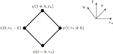
Figure 1: An empty cell never crossed by the particle worldline.

For the cells crossed by the particle, a different integration scheme is imposed, fig. 2. The product potential-wavefunction is given by:

$$\int\!\!\!\!\int_{\tiny Cell}V(r)\Psi dA=V(r)\times$$

$$\left[A_{3}\Psi(t+h,r^{*})+A_{2}\Psi(t-h,r^{*})+A_{4}\Psi(t,r^{*}+h)+A_{1}\Psi(t,r^{*}-h)+{\cal O}(h^{3})\right],$$ (39)

where $A_{1},A_{2},A_{3},A_{4}$ are the sub-surfaces of the cell. The integration of the source term is given by:

$$\int\!\!\!\!\int_{\tiny Cell}SdA=-\int_{t_{i}}^{t_{o}}\frac{2\kappa(r-2M)}{E(2\lambda+1)(\lambda z_{u}+3M)^{2}}\times$$

$$\left[\frac{6M}{z_{u}}(1-E^{2})+\lambda(\lambda+1)-\frac{3M^{2}}{z_{u}^{2}}+\frac{4\lambda M}{z_{u}}\right]dt+\frac{2\kappa(r-2M)}{E(2\lambda+1)(\lambda z_{u}+3M)}\times$$

$$\left\{{Sign_{i}}\left[1+\frac{{Sign_{i}}}{E}\sqrt{\frac{2M}{z_{u}}-\frac{2M}{z_{u0}}}\right]^{-1}+{Sign_{o}}\left[1-\frac{{Sign_{o}}}{E}\sqrt{\frac{2M}{z_{u}}-\frac{2M}{z_{u0}}}\right]^{-1}\right\},$$ (40)

where $t_{i}$ corresponds to the time of entry of the particle in the cell and $t_{o}$ the time of departure from the cell; $z_{u0}$ is the initial position of the particle; $E=\sqrt{1-2M/z_{u0}}$; ${Sign_{i}}=+1$ if the particle enters the cell on the right, $-1$ if on the left; ${Sign_{o}}=+1$ if the particle leaves the cell on the right, $-1$ if on the left, fig. 2. Through the evolution algorithm, the value of $\Psi$ at the upper cell corner is given by:

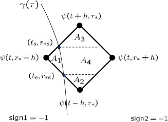
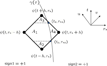
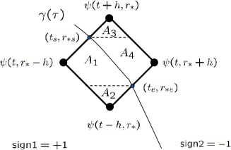
Figure 2: There are only three physical cases for the particle crossing the $t,r$ cell.

$$\Psi(t+h,r^{*})=$$

$$-\Psi(t-h,r^{*})\left[1+\frac{V(r)}{4}(A_{2}-A_{3})\right]+\Psi(t,r^{*}+h)\left[1-\frac{V(r)}{4}(A_{4}+A_{3})\right]+$$

$$\Psi(t,r^{*}-h,)\left[1-\frac{V(r)}{4}(A_{1}+A_{3})\right]-\frac{1}{4}\left(1-\frac{V(r)}{4}A_{3}\right)\int\!\!\!\!\int_{\tiny Cell}S(t,r)dA.$$ (41)

For the value of $\Psi$ at $t=h$, the unavailability of $\Psi$ at $t=-h$, is circumvented by using a Taylor expansion of $\Psi(r^{*},-h)$ for the initial conditions $t=0$:

$$\Psi(r^{*},-h)=\Psi(r^{*},0)-h\frac{\partial\psi}{\partial t}\mid_{t=0}.$$ (42)

The setting of initial conditions constitutes a delicate, technical and largely debated issue. Apart from the technical difficulty in the numerical implementation, it suffices to state how much it is crucial to match the initial radiation conditions, that represent the earlier history of the particle, with its position and velocity. For those $z_{u0}$ starting points which are sufficiently far from the horizon, the errors on the initial conditions are fortunately not relevant at later times.

Another numerical issue is the evaluation of the wavefunction and the perturbations at the position of the particle, but unfortunately not described in the literature and too technical for this book. The wavefunction belongs to the $C^{-1}$ continuity class and the values before and after the particle position are computed and compared to the jump conditions posed on the wavefunction and its derivatives ri10 . Further, it is necessary to obtain the third derivatives of the wavefunction to determine the correction to the geodesic background motion of the particle. Given the second order convergence of the above described algorithm, this isn’t easily achieved without recurring to a fourth order scheme lo05 .

7 Relativistic radial fall affected by the falling mass

7.1 The self-force

It has been addressed in the previous section, that the perturbative two-body problem, involving a black hole and a particle with radiation emission, has been tackled almost 40 years ago. For computation of radiation reaction, it may be worth recalling that before 1997, only pN methods existed in the weak field regime. Indeed, it is only slightly more than a decade, that we possess methods misata97 ; quwa97 for the evaluation of the self-force in strong field for point particles, thanks to concurring situations. On one hand, theorists progressed in understanding radiation reaction and obtained formal prescriptions for its determination and, on the other hand, the appearance of requirements from the LISA (Laser Interferometer Space Antenna) project li for the detection of captures of stars by supermassive black holes (EMRI, Extreme Mass Ratio Inspiral), notoriously affected by radiation reaction.

Such factors, theoretical progress and experiment requirements, have pushed the researchers to turn their efforts in finding an efficient and clear implementation of the theorists prescriptions by tackling the problem in the context of perturbation theory, for which the small mass $m$ corrects the geodesic equation of motion on a fixed background via a factor ${\cal O}(m)$ (for a review, see Poisson depo04 and Barack ba09 ).

Before the appearance of the self-force equation and of the regularisation methods, the main theoretical unsolved problem was represented by the infinities of the perturbations at the particle’s position. After determination of the perturbations through eqs. (26, 31-33), the trajectory of the particle could be corrected simply by requiring it to be a geodesic of the total (background plus perturbations) metric (the Christoffel connection ${\bar{\Gamma}}^{\mu}_{\alpha\beta}$ refers to the full metric):

$$\frac{d^{2}x^{\alpha}}{d\tau^{2}}+{\bar{\Gamma}}^{\alpha}_{\beta\gamma}\,\frac{dx^{\beta}}{d\tau}\,\frac{dx^{\gamma}}{d\tau}=0,$$ (43)

but the perturbation behaves as:

$$h_{\alpha\beta}\sim\frac{1}{\sqrt{\left(g_{\gamma\delta}+u_{\gamma}u_{\delta}\right)\left[x^{\gamma}-z_{u}^{\gamma}(\tau)\right]\left[x^{\delta}-z_{u}^{\delta}(\tau)\right]}},$$ (44)

thus diverging as the inverse of the distance to the particle and imposing a singular behavior to ${\bar{\Gamma}}^{\mu}_{\alpha\beta}$ on the trajectory of the particle. Thus, the small perturbations assumption breaks down near the particle, exactly where the radiation reaction should be computed.

The solution was brought by the self-force equation, formulated in 1997 and baptised MiSaTaQuWa, from the surname first two initials of its discoverers, who determined it using various approaches, all yielding the same formal expression. In the MiSaTaQuWa prescription, the self-force is only well defined in the harmonic (de Donder) dd21 ; dd27 gauge (stemmed from the Lorenz gauge lo67 ) and any departure from it - its relaxation - undermines the validity of the equation of motion.

Mino, Sasaki and Tanaka misata97 used two methods, namely the conservation of the total stress-energy tensor and the matched asymptotic expansion. The former generalises the analysis of DeWitt and Brehme dwbr60 and Hobbs ho68 , consisting in the calculation of the electromagnetic self-force in curved spacetime previously performed in flat space by Dirac di38 . It evaluates the perturbation near the worldline using the Hadamard expansion ha23 of the retarded Green function gr50 ; gr52 ; gr54 . Then, it deduces the equation of motion by imposing the conservation of the rank-two symmetric total stress-energy tensor, via integration of its divergence over the interior of a thin world tube around the particle’s worldline.

The latter, reformulated by Poisson po04 , in a buffer zone matches asymptotically the expansion of the black hole perturbed background by the particle with the expansion around the particle distorted by the black hole.

Also in 1997, the axiomatic approach by Quinn and Wald quwa97 was presented. To them, the self-force is identified by comparison of the perturbation in curved spacetime with the perturbation in flat spacetime. The procedure allows elimination of the divergent part and extraction of the finite part of the force.

On the footsteps of Dirac’s definition of radiation reaction, in 2003 Detweiler and Whiting dewh03 , see also Poisson po04 , offered a novel approach. In flat spacetime, the radiative Green function is obtained by subtracting the singular contribution, half-advanced plus half-retarded, from the retarded Green function. In curved spacetime, and in the gravitational case, the attainment of the radiative Green function passes through the inclusion of an additional, purposely built, function. The singular part does not exert any force on the particle, upon which only the regular field acts de01 . The latter, solely responsible of the self-force, satisfies the homogeneous wave equation and may be considered a radiative field in interaction with the particle. This approach emphasises that the motion is a geodesic of the full metric and it implies two notable features: the regularity of the radiative field and the avoidance of any non-causal behaviour.

Gralla and Wald have attempted a more rigorous way of deriving a gravitational self-force grwa08 . Their final prescription, namely self-consistency versus the first order perturbative correction to the geodesic of the background spacetime, shall be addressed later in this chapter. On the same track of improving rigour, an alternative approach and a new derivation of the self-force have been proposed by Gal’tsov and coworkers gaspst06 and by Pound po10 , respectively.

The determination of the self-force has allowed not only targeted applications geared to more and more complex astrophysical scenarios, but also fundamental investigations: on the role of passive, active and inertial mass by Burko bu05 ; the already quoted papers on the Newtonian self-force depo04 , on the EP dewh03 ; whde03 , on the relation to energy conservation by Quinn and Wald quwa99 ; on the relation between self-force and radiation reaction examined through gauge dependence and adiabaticity by Mino mi05a ; mi05b ; mi05c ; mi06 ; the differentiation between adiabatic, secular and radiative approximations as well as the relevance of the conservative effects by Pound and Poisson popo08 ; on the relation between $h^{\tiny tail}$ and $h^{R}$, tail and regular parts of the field by Detweiler de05 .

The following wishes to be constrained to a physical and sketchy picture of the self-force. For this purpose, the original MiSaTaQuWa approach - the force acts on the background geodesic - is more intuitive. One pictorial description refers to a particle that crosses the curved spacetime and thus generates gravitational waves. These waves are partly radiated to infinity (the instantaneous part) and partly scattered back by the black hole potential (the non-local part), thus forming tails which impinge on the particle and give origin to the self-force. Alternatively, the same phenomenon is described by an interaction particle-black hole generating a field which behaves as outgoing radiation in the wave-zone and thereby extracts energy from the particle. In the near-zone, the field acts on the particle and determines the self-force which impedes the particle to move on the geodesic of the background metric. The total force is thus written as:

$$F^{\alpha}_{full}(x)=F^{\alpha}_{inst.}+F^{\mu}_{tail},$$ (45)

where $F^{\alpha}_{inst.}$ is computed from the contributions that propagate along the past light cone and $F^{\alpha}_{tail}$ has the contributions from inside the past light cone, product of the scattering of perturbations due to the motion of the particle in the curved spacetime created by the black hole, fig. 3 (pictorially, in a curved spacetime, the radiation is not solely confined to the wave front). The self-force is then computed by taking the limit $F^{\mu}_{self}=F^{\mu}_{tail}\left[x\to z_{u}(t)\right]$. Thus, it is conceived as force acting on the background geodesic misata97 ; quwa97 , wherein $\Gamma^{\alpha}_{\beta\gamma}$ refers to the background metric:

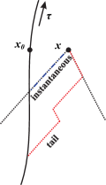
Figure 3: The radiation is going to infinity (instantaneous) or is scattered back (tail). The latter part determines the self-force. The self-force is defined for $x$ to $\rightarrow z_{u}$ where $z_{u}$ is the position of the particle on the worldline $\tau$, while $x$ is the evaluation point.

$$F^{\alpha}_{self}=m\frac{Du^{\alpha}}{d\tau}=\frac{d^{2}x^{\alpha}}{d\tau^{2}}+\Gamma^{\alpha}_{\beta\gamma}u^{\beta}u^{\gamma}.$$ (46)

All MiSaTaQuWa-DeWh approaches produce the same equation for the self-acceleration, given by:

$$a^{\alpha}_{self}=-(g^{\alpha\beta}+u^{\alpha}u^{\beta})\left(\nabla_{\delta}h_{\beta\gamma}^{*}-\frac{1}{2}\nabla_{\beta}h_{\gamma\delta}^{*}\right)u^{\gamma}u^{\delta},$$ (47)

where the star indicates the tail (MiSaTaQuWa) or radiative (DeWh) component. Eq. (47) is not gauge invariant and depends upon the de Donder gauge condition:

$${\tilde{h}}^{\mu\nu\,*}_{;\nu}=0,$$ (48)

where ${\tilde{h}}_{\gamma\delta}^{*}=h_{\gamma\delta}^{*}-\frac{1}{2}g_{\gamma\delta}h^{*}$ and $h^{*}=g^{\mu\nu}h_{\mu\nu}^{*}$. Barack and Ori have shown baor01 that under a coordinate transformation of the form $x^{\alpha}\rightarrow x^{\alpha}-\xi^{\alpha}$, under which the perturbation transforms according to:

$$h_{\mu\nu}\to h_{\mu\nu}+\xi_{\mu;\nu}+\xi_{\nu;\mu},$$ (49)

the self-force acceleration transforms as:

$$a^{\alpha}_{self}\to a^{\alpha}_{self}-\left[(g^{\alpha\lambda}+u^{\alpha}u^{\lambda})\frac{d^{2}{\xi}_{\lambda}}{d\tau^{2}}+R^{\alpha}_{\ \mu\lambda\nu}u^{\mu}\xi^{\lambda}u^{\nu}\right],$$ (50)

where the terms are evaluated at the particle and $R^{\alpha}_{\ \mu\lambda\nu}$ is the Riemann tensor of the background geometry. Thus, for a given two-body system, the MiSaTaQuWa-DeWh acceleration is to be mentioned together with the chosen gauge.

The identification of the tail and instantaneous parts was not accompanied by a prescription of the cancellation of divergencies, which indeed arrived three years later thanks to the mode-sum method by Barack and coworkers baor00 ; ba00 ; ba01 ; babu00 . The mode-sum method relies on solutions to interwoven difficulties, mostly related to the divergent nature of the problem, but tentatively presented as separate hereafter.

Spherical symmetry allows the force to be expanded into spherical harmonics and turns out to be once more the key factor for black hole physics, after having been the expedient for the determination of the wave equation. The divergent nature of the problem is then transformed into a summation problem. For each multipole, the full force is finite and the divergence appears only upon infinite summing over $l,m$.

Furthermore, the tail component can’t be calculated directly, but solely as difference between the full force and the instantaneous part; thus, the self-force is computed as:

$$F_{self}^{\alpha}=\lim_{x\to z_{u}}\sum_{l}\left[F_{full}^{\alpha\,l\pm}(x)-F_{inst.}^{\alpha\,l\pm}(x)\right].$$ (51)

Each of the two quantities $F_{full}^{\alpha\,l}(x)$ and $F_{inst.}^{\alpha\,l}$ is discontinuous through the particle location and the superscript $\pm$ indicates the two (different) values obtained by taking the particle limit from outside ($x\rightarrow z^{+}_{u}$) and inside ($x\rightarrow z^{-}_{u}$). However, the difference in eq. (51) does not depend upon the direction from which the limit is taken.

The full and the instantaneous parts have the same singular behaviour at large $l$ and close to the particle; their difference should be sufficient to ensure a regular behaviour at each $l$. Unfortunately, another obstacle arises from the difficulty of calculating the instantaneous part mode by mode. Therefore, the divergence is dealt with by seeking a function $H^{\alpha\,l}$, such that the series $\sum_{l}\left[F_{full}^{\alpha\,l\pm}-H^{\alpha\,l\pm}\right]$ is convergent.

The function $H^{\alpha\,l}$ mimics the instantaneous component at large $l$ and close to the particle. Once such condition is ensured, eq. (51) is rewritten as:

$$F_{self}^{\alpha}=\sum_{l}\left[F_{full}^{\alpha\,l\pm}-H^{\alpha\,l\pm}\right]-D^{\alpha\,l\pm},$$ (52)

where

$$D^{\alpha\,l\pm}(x)=\lim_{x\to z_{u}}\sum_{l}\left[F_{inst.}^{\alpha\,l\pm}(x)-H^{\alpha\,l\pm}(x)\right].$$ (53)

The addition and subtraction of the function $H^{\alpha\,l}$ guarantees the pristine value of the computation. In general, for $L=l+1/2$:

$$H^{\alpha\,l}=A^{\alpha}\,L+B^{\alpha}+C^{\alpha}/L.$$ (54)

Thus, the mode-sum amounts to ba01 : i) numerical computation of full modes; ii) derivation of the regularisation parameters $A,B,C$, and $D$ (obtained on a local analysis of the Green s function near coincidence, $x\rightarrow z_{u}$, at large l); iii) computation of eq. (52) whose behaviour has to show a $1/L^{2}$ fall off if previous steps are correctly carried out.

7.2 The pragmatic approach

The straightforward pragmatic approach by Lousto, Spallicci and Aoudia lo00 ; lo01 ; sp99 ; spao04 is the direct implementation of the geodesic in the full metric (background + perturbations) and it is coupled to the renormalisation by the Riemann-Hurwitz $\zeta$ function. These two features justify the pragmatic adjective. Though the application of the $\zeta$ function is somewhat artificial and the pragmatic method is somewhat naive, the latter has the merit of: i) a clear identification of the different factors participating in the motion; ii) potential applicability to any gauge and to higher orders of the $\zeta$ function renormalisation.

Dealing only with time and radial components, two geodesic equations can be written and then combined into a single one, after elimination of the geodesic parameter. Thus, for radial fall the coordinate acceleration is given by the sole radial component:

$${\ddot{z}}_{p}={\bar{\Gamma}}_{rr}^{t}{\dot{z}}^{3}_{p}+2{\bar{\Gamma}}_{tr}^{t}{\dot{z}}^{2}_{p}-{\bar{\Gamma}}_{rr}^{r}{\dot{z}}^{2}_{p}+{\bar{\Gamma}}_{tt}^{t}{\dot{z}_{p}}-2{\bar{\Gamma}}_{tr}^{r}{\dot{z}_{p}}-{\bar{\Gamma}}{tt}^{r},$$ (55)

where ${\bar{\Gamma}}^{\alpha}_{\beta\gamma}$ refers to the full metric and $z_{p}$ is given by eq. (56). Eq. (55) refers to:

• the full metric field ${\bar{g}}_{\mu\nu}(t,r)$ previously defined;

• the displacement $\Delta z$, difference between the perturbed $z_{p}(t)$ and the unperturbed $z_{u}(t)$ positions, and the coordinate time derivatives:

  $$z_{p}=z_{u}+\Delta z,~{}~{}~{}~{}~{}~{}~{}~{}~{}~{}~{}~{}~{}~{}{\dot{z}}_{p}={\dot{z}}_{u}+{\Delta\dot{z}},~{}~{}~{}~{}~{}~{}~{}~{}~{}~{}~{}~{}~{}~{}{\ddot{z}}_{p}={\ddot{z}}_{u}+{\Delta\ddot{z}}~{};$$ (56)

• the Taylor expansion of the field and its spatial derivative:

  $${\bar{g}}_{\mu\nu}\mid_{z_{p}}={\bar{g}}_{\mu\nu}\mid_{z_{u}(t)}+\Delta z{\bar{g}}_{\mu\nu,r}\mid_{r=z_{u}(t)},$$

  $${\bar{g}}_{\mu\nu,r}\mid_{z_{p}}={\bar{g}}_{\mu\nu,r}\mid_{z_{u}(t)}+\Delta z{\bar{g}}_{\mu\nu,rr}\mid_{r=z_{u}(t)}.$$ (57)

The unperturbed trajectory of the particle $z_{u}(t)$ is given by the inverse of the relations $T(r)$, e.g. eq. (28). Supposing that the relative strengths of the perturbations and the deviations behave as:

$$\frac{[h^{(1)}]^{2}}{g}\simeq\frac{h^{(2)}}{g}\ll\frac{h^{(1)}}{g}\simeq\frac{\Delta{\dot{z}}}{{\dot{z}}_{p}}\simeq\frac{\Delta z}{z_{p}}.$$ (58)

Then, the coordinate acceleration correction is given by an expansion up to $1^{st}$ order for all quantities, which corresponds to the expression in lo00 ; lo01 :

$$\Delta{\ddot{z}}=\alpha_{1}\left(g,{\dot{z}}_{u}\right)\Delta z+\alpha_{2}\left(g,{\dot{z}}_{u}\right)\Delta{\dot{z}}+\alpha_{6}\left(h,{\dot{z}}_{u}\right).$$ (59)

The particle determines in first instance the emission of radiation $h_{\alpha\beta}$, which after backscattering by the black hole potential, interacts with the particle itself resulting into a change in acceleration (the coefficient $\alpha_{6}$ depending on $h_{\mu\nu}$ and derivatives). The latter places the particle elsewhere from where it should have been, that is $z_{u}(t)$. The field is thus to be evaluated at this new position resulting into a further variation in acceleration (the terms $\alpha_{1}\Delta z$ and $\alpha_{2}\Delta{\dot{z}}$ depending on $g_{\mu\nu}$ and derivatives).

All terms in eqs. (59, 62) are of $1/M$ order; the terms $\alpha_{1}\Delta z$ and $\alpha_{2}\Delta{\dot{z}}$ represent the background field evaluated on the perturbed trajectory; $\alpha_{6}$ represents the perturbed field on the background trajectory. The expressions in tab.1 are gauge independent, while in tab.2 they are shown in the Regge-Wheeler gauge ($H_{0}=H_{2}$ and $K=0$ as in head-on geodesics). Finally, the coefficient $\alpha_{0}$ is the lowest order term corresponding to a particle radially falling into the SD black hole and not affected by the perturbations. It corresponds to the unrenormalised acceleration and it is to be added to the terms of eqs. (59,62) to compute the total acceleration:

$$\alpha_{0}=g^{tt}g_{tt,r}\dot{z}_{u}^{2}-\frac{1}{2}g^{rr}g_{rr,r}\dot{z}_{u}^{2}+\frac{1}{2}g^{rr}g_{tt,r}=\displaystyle-\frac{M}{r^{2}}\left[1-\frac{2M}{r}-3\left(1-\frac{2M}{r}\right)^{-1}\dot{z}_{u}^{2}\right].$$ (60)

If $\Delta{\ddot{z}}$ receives its main contribution from the background metric $g_{\mu\nu}$ or else cumulative effects are let to grow, a different expansion may be considered.

Table 1: Representation of the terms of eq. (59) in gauge independent form. The elements in each column are produced by the terms of eq. (55), in the first row. From the algebraic sum of the elements between horizontal lines, the terms of eq. (59) are derived.

	${\bar{\Gamma}}_{rr}^{t}{\dot{z}}^{3}_{p}$	$2{\bar{\Gamma}}_{tr}^{t}{\dot{z}}^{2}_{p}$	$-{\bar{\Gamma}}_{rr}^{r}{\dot{z}}^{2}_{p}$	${\bar{\Gamma}}_{tt}^{t}{\dot{z}}_{p}$	$-2{\bar{\Gamma}}_{tr}^{r}{\dot{z}}_{p}$	$-{\bar{\Gamma}}_{tt}^{r}$
$\alpha_{1}\Delta z$		$g^{tt}_{,r}g_{tt,r}\dot{z}_{u}^{2}\Delta z$	$-\frac{1}{2}g^{rr}_{,r}g_{rr,r}\dot{z}_{u}^{2}\Delta z$			$\frac{1}{2}g^{rr}_{,r}g_{tt,r}\Delta z$
		$g^{tt}g_{tt,rr}\dot{z}_{u}^{2}\Delta z$	$-\frac{1}{2}g^{rr}g_{rr,rr}\dot{z}_{u}^{2}\Delta z$			$\frac{1}{2}g^{rr}g_{tt,rr}\Delta z$
$\alpha_{2}\Delta\dot{z}$		$2g^{tt}g_{tt,r}\dot{z}_{u}\Delta\dot{z}$	$-g^{rr}g_{rr,r}\dot{z}_{u}\Delta\dot{z}$
$\alpha_{6}$	$g^{tt}h_{tr,r}\dot{z}_{u}^{3}$	$-h^{tt}g_{tt,r}\dot{z}_{u}^{2}$	$\frac{1}{2}h^{rr}g_{rr,r}\dot{z}_{u}^{2}$	$\frac{1}{2}g^{tt}h_{tt,t}\dot{z}_{u}$	$-g^{rr}h_{rr,t}\dot{z}_{u}$	$-g^{rr}h_{tr,t}$
	$-\frac{1}{2}g^{tt}h_{rr,t}\dot{z}_{u}^{3}$	$g^{tt}h_{tt,r}\dot{z}_{u}^{2}$	$-\frac{1}{2}g^{rr}h_{rr,r}\dot{z}_{u}^{2}$	$\frac{1}{2}h^{tr}g_{tt,r}\dot{z}_{u}$	$h^{tr}g_{tt,r}\dot{z}_{u}$	$-\frac{1}{2}h^{rr}g_{tt,r}$
	$-\frac{1}{2}h^{tr}g_{rr,r}\dot{z}_{u}^{3}$					$\frac{1}{2}g^{rr}h_{tt,r}$

Table 2: Representation of the terms of eq. (59) in Regge-Wheeler gauge. The elements in each column are produced by the terms of eq. (55), in the first row. From the algebraic sum of the elements between horizontal lines, the terms of eq. (59) are derived.

$\alpha_{1}\Delta z$	$\displaystyle-\frac{M}{r^{2}}\left[{\displaystyle\frac{6M}{r^{2}}}-\frac{2}{r}+{\displaystyle\frac{6(r-M)}{r^{2}}\left(1-\frac{2M}{r}\right)^{-2}}\dot{z}_{u}^{2}\right]\Delta z$
$\alpha_{2}\Delta\dot{z}$	${\displaystyle\frac{6M}{r^{2}}\left(1-\frac{2M}{r}\right)^{-1}}\dot{z}_{u}\Delta\dot{z}$
$\alpha_{6}$	$\displaystyle\frac{1}{r-2M}\left[\frac{r^{2}H_{0,t}}{2(r-2M)}-\displaystyle\frac{MH_{1}}{r-2M}-rH_{1,r}\right]\dot{z}_{u}^{3}-\displaystyle\frac{3}{2}H_{0,r}\dot{z}_{u}^{2}-3\left({\displaystyle\frac{H_{0,t}}{2}}-{\displaystyle\frac{MH_{1}}{r^{2}}}\right)\dot{z}_{u}$
	$+{\displaystyle\frac{r-2M}{r}}\left[{\displaystyle\frac{2MH_{0}}{r^{2}}}+{\displaystyle\frac{(r-2M)H_{0,r}}{2r}}-H_{1,t}\right]$

In radial fall, it has been indicated by two different heuristic arguments lo00 ; lona09 that the metric perturbations should be of $C^{0}$ continuity class at the location of the particle. One argument lo00 is based on the integration over $r$ of the Hamiltonian constraint, which is the $tt$ component of the Einstein equations (eq.[C7a] in ze70c ); the other lona09 on the structure of selected even perturbations equations. In aosp10a , a stringent analysis on the $C^{0}$ continuity is pursued in terms of the jump conditions that the wavefunctions and derivatives have to satisfy to guarantee the continuity of the perturbations. Anyhow, the connection coefficients and the metric perturbation derivatives have a finite jump and they can be computed as the average of their values at $z_{u}\pm\epsilon$ with $\epsilon\to 0$.

The supposed $C^{0}$ continuity class of the metric perturbations allows to deal with the divergence with $l$ of the $\alpha_{6}$ coefficient lo00 ; lo01 . The divergence originates from the infinite sum over the finite multipole component contributions. One way of regularising this sum is to subtract to each mode precisely the $l\to\infty$ contribution, since for ever larger $l$ the metric perturbations tend to some finite asymptotic behaviour. Thus, the subtraction from each mode of the $l\rightarrow\infty$ part leads to a convergent series. The renormalisation by the Riemann-Hurwitz $\zeta$ function was proposed first in lo00 ; lo01 and then extended to higher orders in spao04 . For $L=l+1/2$, it can be shown that:

$$\alpha_{6}=\sum_{l=0}^{\infty}\alpha_{6}^{l},~{}~{}~{}~{}~{}~{}~{}~{}~{}~{}~{}~{}~{}\alpha_{6}^{l}=\alpha_{6\pm}^{a}L+\alpha_{6}^{b}L^{0}+\alpha^{c}_{6\pm}L^{-1}+\alpha_{6}^{d}L^{-2}+{\cal O}(L^{-3}).$$ (64)

Eq. (64) is casted to have a similar form to the mode-sum expression. The average of $\alpha^{a}_{6\pm}$ and $\alpha^{c}_{6\pm}$ vanish at the position of the particle, whereas $\sum_{l=0}^{\infty}\alpha_{6}^{b}=\infty$ determines the divergence.

The Riemann $\zeta$ function ri59 and its generalisation, the Hurwitz $\zeta$ function hu82 , are defined by:

$$\zeta(s)=\sum_{l=1}^{\infty}(l)^{-s},~{}~{}~{}~{}~{}~{}~{}~{}~{}~{}~{}~{}~{}\zeta(s,a)=\sum_{l=0}^{\infty}(l+a)^{-s},$$ (65)

where in our case $a=1/2$. Two special values of the Hurwitz functions, namely $\zeta(0,1/2)=0$ and $\zeta(2,1/2)=1/2~{}\pi^{2}$, cancel the divergent term and determine that the term $\sum_{l=0}^{\infty}\alpha_{6}^{d}L^{-2}$ gets a finite value, respectively. Barack and Lousto balo02 have shown the concordance of the mode-sum and the $\zeta$ regularisations for radial fall.

8 The state of the art

It is now time to discuss the state of the art of the radial fall affected by its mass and the emitted radiation. As shown in the introduction, the adiabatic approximation requires that a given orbital parameter $q$ changes slowly over time scales comparable to the orbital period $P$ (this is somewhat a coarse definition since the small mass always ‘reacts’ immediately): $\Delta q={\dot{q}}P\ll q$. For circular and moderately elliptic orbits, the above condition, where $q$ is function of the semi-lactus rectum $p$ and eccentricity $e$, is transformed into a condition on the $m/M$ ratio cukepo94 . In radial fall, though, it is far from being evident, and even possible, to identify a condition on adiabaticity within which any simplification may occur. The feebleness of cumulative effects for radiation reaction does not imply their non-existence. On the contrary, this is the case where most care and sophisticated techniques are demanded for the computation of the motion affected by the back-action, even if the latter has moderate effects. Therefore it is not surprising, thanks to the feebleness and to the difficulties, that solely two studies (one based on the pragmatic method, the other on the self-force) exist.

8.1 Trajectory

The perennial question on the behaviour of the infalling mass reflects itself in the determination along which direction the back-action is exerted.

Lousto (fig. 2a in lo00 ) suggests that the $\alpha_{6}$ term, denoted therein $C$ (the variation of the coordinate acceleration of the particle due solely to perturbations; it corresponds to the self-force when referred to coordinate time, see next section), increases approaching the Zerilli potential at $3.1M$ and reaches its peak value around $2.4M$. The same reference (fig. 2b in lo00 ) shows that the coordinate acceleration, thus including $\alpha_{1}\Delta z$ and $\alpha_{2}\Delta{\dot{z}}$ terms, is slowed down and mostly until around $3.1M$. The two statements are not contradictory if the discrepancy is attributed to $\alpha_{1}\Delta z$ and $\alpha_{2}\Delta{\dot{z}}$. In the same reference lo00 , deceleration is expected as the system is losing energy and momentum. This repulsive behaviour - before the Zerilli potential peak - is confirmed in the abstract of lo01 .

Conversely, for Barack and Lousto balo02 the radial component of the self-force is found to point inward (i.e., toward the black hole) throughout the entire plunge, independently on the starting point $z_{u0}$. The work done by the self-force is considered positive, resulting in an increase of the energy parameter $E$ throughout the plunge. To these results, it is attached a specific gauge choice (as opposed to the energy flux at infinity, which is gauge invariant) balo02 .

The upward or inward direction impressed on the particle by its mass and the emitted radiation and whether this direction is maintained throughout the plunge or part of it, is a fundamental if not the main one, feature to acquire in such analysis. Again here, the statements from the three papers might not be contradictory as Lousto lo00 ; lo01 describes motion in coordinate Schwarzschild time, and includes geodesic deviations. Conversely, Barack and Lousto balo02 describe motion in proper time and apply only the self-force without geodesic deviations. Nevertheless, it is of interest to remark that the concept of repulsion resurfaces again solely in coordinate time as in the elder debate. The coefficient of the geodesic deviation coefficient $\alpha_{1}$ changes sign during fall, while it does not occur to $\alpha_{2}$ aosp10b which remains negative throughout.

For a particle starting from rest at a finite distance from the black hole, an analytic approximation of the self-force for the $l\geq 2$ modes (while for $l=0,1$ the solutions in ze70c are mentioned) is given by Barack and Loustobalo02 :

$$F_{self}^{r}=F_{self}^{r\,l=0}+F_{self}^{r\,l=1}+\sum_{l=2}^{\infty}\left\{-\frac{15}{16}m^{2}\frac{E^{2}}{r^{2}}\left(E^{2}+\frac{4M}{r}-1\right)\frac{1}{L^{2}}+{\cal O}(L^{-4})\right\},$$ (66)

where $E$ is the orbital energy of the particle. The force has only negative and even powers of $l$, which makes the sum quickly convergent and provides an excellent approximation for the numerical evaluation of the first few lower multipoles. The derivation of such net expression for the self-force is not described in balo02 .

8.2 Regularisation parameters

Regularisation parameters of the mode-sum method have been confirmed independently by different papers ba01 ; baminaorsa02 and they are consistent with the results obtained by the application of the $\zeta$ function balo02 . In radial fall, there is a regular gauge transformation between the de Donder and Regge-Wheeler gauges baor01 , and thus the regularisation parameters were also determined in the latter gauge ao08 ; balo02 . The results are:

$$A_{\pm}^{r}=\mp\frac{m^{2}}{z_{u}^{2}}\,E,~{}~{}~{}~{}~{}~{}~{}~{}~{}~{}~{}~{}A_{\pm}^{t}=\mp\frac{m^{2}}{z_{u}^{2}}\,\frac{\dot{r}_{p}}{f},~{}~{}~{}~{}~{}~{}~{}~{}~{}~{}~{}~{}A_{\pm}^{\theta}=A_{\pm}^{\varphi}=0,$$ (67)

$$B^{r}=-\frac{m^{2}}{2z_{u}^{2}}\,E^{2},~{}~{}~{}~{}~{}~{}~{}~{}~{}~{}~{}B^{t}=-\frac{m^{2}}{2z_{u}^{2}}\,\frac{E\dot{r}_{p}}{f},~{}~{}~{}~{}~{}~{}~{}~{}~{}~{}~{}~{}B^{\theta}=B^{\varphi}=0,$$ (68)

$$C^{\alpha}=D^{\alpha}=0,$$ (69)

where $f\equiv 1-2M/z_{u}$ and ${\dot{z}}_{u}=-(E^{2}-f)^{1/2}$.

8.3 Effect of radiation reaction on the waveforms during plunge

Thanks to a suggestion of B. Whiting, preliminary indications were found ao08 . The waveforms shifts are of the order of (tens of) seconds for a particle sensibly radiating for few thousands of seconds, having started at rest from a finite distance between $4M$ and $40M$. The assumption used therein is energy-momentum balance (the energy radiated to infinity and absorbed by the black hole is imposed to be equal to the energy change in the particle fall). This assumption is likely jeopardised by the lack of instantaneous energy conservation quwa99 .

The correct alternative is the computation of the self-force and its continuous implementation all along the trajectory. It is thus mandatory to consider the application of the recently proposed self-consistent prescription grwa08 , unfortunately not yet part of the state of the art in terms of its application.

9 Beyond the state of the art: the self-consistent prescription

In grwa08 a rigorous derivation and application of the self-force equation is proposed. In the derivation, emphasis is put upon the de Donder gauge and the consequences of relaxation, that is not enforcing this gauge. On one hand, the de Donder gauge is imposed by the nature of the self-force, solely defined in this gauge. On the other hand, the relaxation of the de Donder gauge stems from the need of departing from the background geodesic to find the self-force that causes such departure. Previous derivations were based on the assumption of deviations from geodesic motion expected to be small; by consequence, the de Donder gauge violation should likewise be small. Instead, the new derivation by Gralla and Wald is a rigorous, perturbative, result, obtained without the step of de Donder gauge relaxation and containing the geodesic deviation terms.

But Gralla and Wald go a step further grwa08 . For the evolution of an orbit, rather than a first order perturbation equation containing geodesic deviation terms, they recommend a self-consistent approach. Such prescription basically affirms the greater accuracy of a first order perturbation expansion along a continuously corrected trajectory as opposed to a higher order perturbation expansion made on the background geodesic. Self-consistency bypasses the issue of relaxation, since at each integration step a new geodesic is found.

The ‘classic’ first order perturbative expansion for the motion of a small body determines that the first order metric perturbations satisfy:

$$\nabla^{\gamma}\nabla_{\gamma}\tilde{h}_{\alpha\beta}-2R^{\gamma}{}_{\alpha\beta}{}^{\delta}\tilde{h}_{\gamma\delta}=-16\pi Mu_{\alpha}u_{\beta}\frac{\delta^{(3)}(x^{\mu})}{\sqrt{-g}}\frac{d\tau}{dt},$$ (70)

where $x^{\mu}=0$ corresponds to a geodesic $\gamma$ of the background spacetime, and $u^{\alpha}$ is the tangent to $\gamma$. It is reminded that $\tilde{h}_{\alpha\beta}\equiv h_{\alpha\beta}-\frac{1}{2}hg_{\alpha\beta}$ with $h=h_{\alpha\beta}g^{\alpha\beta}$. For a retarded solution to this equation (thus satisfying the de Donder gauge condition) of the type:

$$h_{\alpha\beta}^{\tiny\textrm{tail}}(x)=M\int_{-\infty}^{\tiny\tau_{\textrm{ret}}^{-}}\left(G^{+}_{\alpha\beta\alpha^{\prime}\beta^{\prime}}-\frac{1}{2}g_{\alpha\beta}G^{+\gamma}_{\gamma\alpha^{\prime}\beta^{\prime}}\right)\left[x,z_{u}(\tau^{\prime})\right]u^{\alpha^{\prime}}u^{\beta^{\prime}}d\tau^{\prime},$$ (71)

the first order in $\lambda$ deviation of the motion from $\gamma$ is expressed by (see grwa08 for the additional spin term):

$$u^{\gamma}\nabla_{\gamma}(u^{\beta}\nabla_{\beta}Z^{\alpha})=-{R_{\beta\gamma\delta}}^{\alpha}u^{\beta}Z^{\gamma}u^{\delta}-(g^{\alpha\beta}+u^{\alpha}u^{\beta})(\nabla_{\delta}h_{\beta\gamma}^{\tiny\textrm{tail}}-\frac{1}{2}\nabla_{\beta}h_{\gamma\delta}^{\tiny\textrm{tail}})u^{\gamma}u^{\delta}.$$ (72)

Self-consistency prescribes that rather than using eqs. (70,71,72), it is instead preferable to apply the self-force coherently all along the trajectory:

$$\nabla^{\gamma}\nabla_{\gamma}\tilde{h}_{\alpha\beta}-2R^{\gamma}{}_{\alpha\beta}{}^{\delta}\tilde{h}_{\gamma\delta}=-16\pi Mu_{\alpha}(t)u_{\beta}(t)\frac{\delta^{(3)}\left[x^{\mu}-z^{\mu}_{p}(t)\right]}{\sqrt{-g}}\frac{d\tau}{dt},$$ (73)

$$u^{\beta}\nabla_{\beta}u^{\alpha}=-(g^{\alpha\beta}+u^{\alpha}u^{\beta})(\nabla_{\delta}h_{\beta\gamma}^{\tiny\textrm{tail}}-\frac{1}{2}\nabla_{\beta}h_{\gamma\delta}^{\tiny\textrm{tail}})u^{\gamma}u^{\delta},$$ (74)

$$h_{\alpha\beta}^{\tiny\textrm{tail}}(x)=M\int_{-\infty}^{\tiny\tau_{\textrm{ret}}^{-}}\left(G^{+}_{\alpha\beta\alpha^{\prime}\beta^{\prime}}-\frac{1}{2}g_{\alpha\beta}G^{+\gamma}_{\gamma\alpha^{\prime}\beta^{\prime}}\right)\left[x,z_{p}(\tau^{\prime})\right]u^{\alpha^{\prime}}u^{\beta^{\prime}}d\tau^{\prime},$$ (75)

where this time $u^{\alpha}(\tau)$ in eqs. (74,75), normalised in the background metric, refers to the self-consistent motion $z_{p}(\tau)$, rather than to a background geodesic as in eqs. (71,72); $G^{+}_{\alpha\beta\alpha^{\prime}\beta^{\prime}}$ is the retarded Green function, normalised with a factor of $-16\pi$ quwa97 ; the symbol $\tau_{\tiny\textrm{ret}}^{-}$ indicates the range of the integral being extended just short of the retarded time $\tau_{\tiny\textrm{ret}}$, so that only the interior part of the light-cone is used.

The geodesic deviations vanish in eq. (74), since self-consistency is imposed. Nevertheless, there might be situations where, for a whatever reason, the numerical implementation of the self-consistent prescription may be cumbersome. In this case, the addition of geodesic deviation terms might as in eq. (72) be necessary.

If furthermore, motion is wished to be expressed in coordinate time, like in the pragmatic approach, it is useful to find a correspondence between the first order perturbation equation, containing geodesic deviations, eq. (72), and the terms of eq. (59). It is going to be shown that the $\alpha_{6}$ term of eqs. (59, 62) corresponds to the self-force term of eq. (72), when the latter is transferred to coordinate time. Referring to the time and radial components of the self-force, it is obtained from eqs. (46, 47):

$$\frac{d^{2}t}{d\tau^{2}}=F^{t}_{self}-m\Gamma^{t}_{\beta\gamma}u^{\beta}u^{\gamma}=-mg^{t\beta}\left(h^{*}_{\beta\gamma\,;\delta}-\frac{1}{2}h^{*}_{\gamma\delta\,;\beta}\right)u^{\gamma}u^{\delta}-mk^{t},$$ (76)

$$\frac{d^{2}r}{d\tau^{2}}=F^{r}_{self}=-m\Gamma^{r}_{\beta\gamma}u^{\beta}u^{\gamma}-mg^{r\beta}\left(h^{*}_{\beta\gamma\,;\delta}-\frac{1}{2}h^{*}_{\gamma\delta\,;\beta}\right)u^{\gamma}u^{\delta}-mk^{r},$$ (77)

where

$$k^{\alpha}=\left(h^{*}_{\beta\gamma\,;\delta}-\frac{1}{2}h^{*}_{\delta\gamma\,;\beta}\right)u^{\alpha}u^{\beta}u^{\gamma}u^{\delta}.$$ (78)

Since:

$$\frac{d}{d\tau}=\frac{dt}{d\tau}\frac{d}{dt}~{}~{}~{}~{}~{}~{}~{}~{}~{}~{}~{}\frac{d^{2}r}{d\tau^{2}}=\frac{dr}{dt}\frac{d^{2}t}{d\tau^{2}}+\frac{d^{2}r}{dt^{2}}\left(\frac{dt}{d\tau}\right)^{2},$$

after some computation, the term $k^{\alpha}$ disappears when the self-force is expressed in coordinate time:

$$m\frac{d^{2}r}{dt^{2}}=m\left[\Gamma^{t}_{\beta\gamma}v^{\beta}v^{\gamma}+g^{t\beta}\left(h^{*}_{\beta\gamma\,;\delta}-\frac{1}{2}h^{*}_{\gamma\delta\,;\beta}\right)v^{\gamma}v^{\delta}\right]{\dot{z}_{u}(t)}$$

$$-m\Gamma^{r}_{\beta\gamma}v^{\beta}v^{\gamma}-mg^{r\beta}\left(h^{*}_{\beta\gamma\,;\delta}-\frac{1}{2}h^{*}_{\gamma\delta\,;\beta}\right)v^{\gamma}v^{\delta}.$$ (79)

Furthermore, a tedious computation shows that eq. (79) is nothing else than the $\alpha_{6}$ term of eq. (59) apart from the regularisations by mode-sum or Riemann-Hurwitz $\zeta$ function:

$$\alpha_{6}\leftrightarrow g^{t\beta}\left(h^{*}_{\beta\gamma\,;\delta}-\frac{1}{2}h^{*}_{\gamma\delta\,;\beta}\right)v^{\gamma}v^{\delta}{\dot{z}_{u(t)}}-g^{r\beta}\left(h^{*}_{\beta\gamma\,;\delta}-\frac{1}{2}h^{*}_{\gamma\delta\,;\beta}\right)v^{\gamma}v^{\delta}.$$ (80)

The recasting of the Riemann tensor term and of the left-hand side of eq. (72) into coordinate time determines the relation to the $\alpha_{1}\Delta z$ and $\alpha_{2}\Delta{\dot{z}}$ terms in eqs. (59, 62). Finally, the geodesic deviation equation eq. (72), is dealt with by Aoudia and Spallicci aosp10b as difference between background and perturbed motions.

10 Conclusions

It has been shown that free fall is still the arena for a deeper comprehension of gravitation. Furthermore, it still generates acute observations like relativistic gliding for which the asymmetric oscillations of a quasirigid body slow down or accelerate its fall in a gravitational background gumo07 .

But is the problem of radial fall solved? Do we know the laws of motion of a star falling into a black hole, the relativistic modern version of the falling stone? A fair and objective answer leads to a moderate optimism. The general relativistic problem has had undeniable progress from 1997, but a careful analysis of the literature shows that some issues are either still partly open or simply not fully at hand, in terms of clear procedures, by means of which clearly cut answers are obtained.

The remaining steps to be fulfilled for a satisfactory level of comprehension for radial fall of a small particle into a large mass (represented by a SD black hole) within the first perturbative order in $m/M$ are divided in three groups.

Investigations to be pursued before recurring to the self-consistent prescription:

1. Compute in proper time the first order perturbation equation with deviation terms, i.e. all terms of eq. (72).

2. Identify and compare expressions for renormalised, semi-renormalised and unrenormalised accelerations in the SD perturbed geometry; evaluate repulsive effects. The last century debate on repulsion has not addressed the effects of mass finitude ($l=0,1$) and radiation reaction on the motion ($l\geq 2$). The inclusion of perturbations blurs the issue further and renders it more complex.

3. Compare the waveform corrections obtained with energy-balance by Aoudia ao08 with those to be obtained by the integration in the equation of motion of the approximate analytic expression of the self-force of Barack and Lousto balo02 . The comparison is of interest only in case of concurring outcomes, as both procedures have a large degree of approximation. An other comparison sp09 could be made with the numerical results for a 10 : 1 mass ratio, as larger mass ratios imply the solution of the numerical two-scale problem, not yet at hand.

4. Solve the initial conditions for particles with non-null or even relativistic initial velocities with and without large eccentricities. If the outcome of the previous item is successful, coarsely identify possible signatures of radiation reaction. It is likely that a non-null initial velocity would act as an amplifier of the waveform shifts due to radiation reaction. In lopr97a , Lousto and Price show that the energy radiated by a non-null initial velocity may rise up to almost two orders of magnitude (see also fig. 3 in lo97 ). Incidentally, this line of work is confluent with the interests shown recently in the particle physics community ardodsto08 ; spcaprbego08 ; shokya08 ; ve10 ; yosh09 for head-on collisions and the associated radiation reaction gakospto10a ; gakospto10b . Hopefully, progress in numerical relativity may lead to analysis of larger mass ratios and thereby test future results of perturbation theory in the range beyond $10^{-3}$.

   Investigations to be performed solely by the implementation of the self-consistent prescription:

5. Evaluate the trajectory by means of the Gralla and Wald self-consistent method grwa08 . At each integration step, for a given number of modes: evaluation of the perturbation functions at the position of the particle; regularisation by mode-sum or $\zeta$ methods; correction of the geodesic and identification of the cell crossed by the particle; computation of the source term; reiteration of the above. Perturbations and self-force analysis in de Donder’s gauge are on-going balo05 ; basa10 .

6. Repeat steps 1-4 on the basis of the acquired self-consistent trajectory. An iterative scheme may be envisaged also in coordinate time.

   Investigations to be performed independently from the self-consistent prescription:

7. Identify whether in a thought radial fall experiment, there is a physical observable independent of the gauge choice or else manifesting a recognisable effects in a given gauge, following Detweiler de08 .

8. Identify the domain of applicability of the self-force. Although self-consistency represents a closer description to perturbed motion, it is limited to cases where local deviations are small, since after all, it remains a perturbative approach. Thus, a quantitative identification of the domain of applicability of such prescription would be of interest to the community developing LISA templates. The adiabatic approximation can’t be evoked to establish the limits of any self-force based analysis. Indeed, the hypothesis on the feeble magnitude of local deviations may be less constraining than the adiabatic hypothesis, for the absence of requirements on averaging. An explicit condition, referring to the geometry of the orbit and to the mass ratio and defining the domain of applicability of the self-force versus fully numerical approaches, is not yet available.

9. Investigate other gauges than Regge-Wheeler and other methods than the self-force for radial fall. A confirmation of the results by Barack, Lousto in lo01 ; balo02 by an independent group is missing, though in ao08 the necessary basic tools are developed, e.g. a numerical programme confirming the waveforms of lopr97b ; mapo02 . It would be also beneficial to carry out an analysis by the EOB method da09b .

The self-force community and even more the EMRI community are animated by different interests ranging from fundamental physics and theory, to numerical applications, data analysis and astrophysics. To these variegated communities and generally to physicists and astrophysicists, the capture of stars by supermassive black holes will bring a development comparable to the ancient markings made by the leaning Pisa tower, the Cambridge apple tree and the Einstein lift.

- (1) C. Allègre, Un peu de science pour tout le monde (Fayard, Paris, 2003).
- (2) S. Antoci, in Meteorological and Geophysical Fluid Dynamics (a book to commemorate the centenary of the birth of Hans Ertel), W. Schröder Ed., 343 (Science Edition, Bremen, 2004).
- (3) S. Antoci, D.-E. Liebscher, Astron. Nachr., 322, 137 (2001).
- (4) Apollo 15, http://nssdc.gsfc.nasa.gov/planetary/lunar/apollo.html
- (5) S. Aoudia, Capture des étoiles par les trous noirs et ondes gravitationnelles, Doctorate thesis, Dir. A.D.A.M. Spallicci, Université de Nice-Sophia Antipolis (2008).
- (6) S. Aoudia, A.D.A.M. Spallicci, in 12th Marcel Grossmann Meeting, Paris 12-18 July 2009, T. Damour, R.T. Jantzen Eds., R. Ruffini Series Ed. (World Scientific, Singapore, to appear).
- (7) S. Aoudia, A.D.A.M. Spallicci, to appear.
- (8) R.F. Aranha, H.P. de Oliveira, I. Damião Soares, E.V. Tonini, Int. J. Mod. Phys. D, 17, 2049 (2008).
- (9) L.I. Arifov, Problemy Teor. Gravitatsii i Èlement. Chastits, 11, 96 (1980).
- (10) L.I. Arifov, Izv. Vyssh. Uchebn. Zaved. Fiz., 4, 61 (1981). English translation: Russian Phys. J., 24, 346 (1981).
- (11) Aristotélēs, Corpus Aristotelicum: Physica (184a), De cælo (268a), Methaphysica (980a), in Latin (in parenthesis the Bekker index). English translation: The complete works of Aristotle, J. Barnes Ed. (Princeton Univ. Press, Princeton, 1984).
- (12) R. Baierlein, Phys. Rev. D, 8, 4639 (1973).
- (13) L. Barack, Phys. Rev. D, 62, 084027 (2000).
- (14) L. Barack, Phys. Rev. D, 64, 084021 (2001).
- (15) L. Barack, Class. Q. Grav., 26, 213001 (2009).
- (16) L. Barack, L. Burko, Phys. Rev. D, 62, 084040 (2000).
- (17) L. Barack, C. Cutler, Phys. Rev. D, 70, 122002 (2004).
- (18) L. Barack, C.O. Lousto, Phys. Rev. D, 66, 061502 (2002).
- (19) L. Barack, C.O. Lousto, Phys. Rev. D, 72, 104026 (2005).
- (20) L. Barack, A. Ori, Phys. Rev. D, 61, 061502 (2000).
- (21) L. Barack, A. Ori, Phys. Rev. D, 64, 124003 (2001).
- (22) L. Barack, Y. Mino, H. Nakano, A. Ori, M. Sasaki, Phys. Rev. Lett., 88, 091101 (2002).
- (23) L. Barack, N. Sago. arXiv:1002.2386v1 (2010).
- (24) H. Bauer, Mathematische Einführung in die gravitationstheorie Einsteins, nebst einer exakten darstellung ihrer wichtigsten ergebnisse (F. Deuticke, Leipzig and Wien, 1922).
- (25) M. Biezunski, Einstein à Paris: le temps n’est plus (Presse Univ. de Vincennes, St. Denis, 1991).
- (26) L. Blanchet, S. Detweiler, A. Le Tiec, B.F. Whiting, Phys. Rev. D, 81, 064004 (2010).
- (27) L. Blanchet, S. Detweiler, A. Le Tiec, B.F. Whiting, Phys. Rev. D, 81, 084033 (2010).
- (28) L. Burko, Class. Q. Grav., 22, S847 (2005).
- (29) A. Cădez̆, M. Calvani, A. Gomboc, U. Kostić, in A. Einstein Century Int. Conf., Paris 18-22 July 2005, AIP Conf. Proc., 861, 566 (2006).
- (30) G. Cavalleri, G. Spinelli, Lett. N. Cim., 6, 5 (1973).
- (31) G. Cavalleri, G. Spinelli, Phys. Rev. D, 15, 3065 (1977).
- (32) S. Chandrasekhar, Proc. R. Soc. London A, 343, 289 (1975).
- (33) S. Chandrasekhar, The mathematical theory of black holes (Oxford Univ. Press, New York, 1983).
- (34) S. Chandrasekhar, S. Detweiler, Proc. R. Soc. London A, 344, 441 (1975).
- (35) K.P. Chung, N. Cim. B, 14, 293 (1973).
- (36) I. Ciufolini, Phys. Rev. D, 34, 1014 (1986).
- (37) I. Ciufolini, J.A. Wheeler, Gravitation and inertia (Princeton Univ. Press, Princeton, 1995).
- (38) F.I. Copperstock, Phys. Rev. D, 10, 3171 (1974).
- (39) P. Crawford, I. Tereno, Gen. Rel. Grav., 34 (2002).
- (40) G. Cruciani, N. Cim. B, 115, 693 (2000).
- (41) G. Cruciani, N. Cim. B, 120, 1045 (2005).
- (42) C. Cutler, D. Kennefick D., E. Poisson, Phys. Rev. D, 50, 3816 (1994).
- (43) M. Dafermos, I. Rodnianski, in Clay Summer School, Zurich 23 June - 18 July 2008, arXiv:0811.0354v1 [gr-qc].
- (44) T. Damour, Sp. Sc. R., 148, 191 (2009).
- (45) T. Damour, arXiv:0910.5533v1 [gr-qc].
- (46) M. Davis, R. Ruffini, N. Cim. Lett., 2, 1165 (1972).
- (47) M. Davis, M., R. Ruffini, W.H. Press, R.H. Price, Phys. Rev. Lett., 27, 1466 (1971).
- (48) M. Davis, R. Ruffini, J. Tiomno, Phys. Rev. D, 5, 2932 (1972).
- (49) T. de Donder, La gravifique Einsteinienne (Gauthier-Villars, Paris, 1921).
- (50) T. de Donder, The mathematical theory of relativity (M.I.T. Press, Cambridge, 1927).
- (51) C. de Jans, Mem. Acad. Roy. Belgique Cl. Sci., 7, 1 (1923).
- (52) C. de Jans, Mem. Acad. Roy. Belgique Cl. Sci., 7, 1 (1924).
- (53) C. de Jans, Mem. Acad. Roy. Belgique Cl. Sci., 7, 96 (1924).
- (54) S. Detweiler, Phys. Rev. Lett., 86, 1931 (2001).
- (55) S. Detweiler, Class. Q. Grav., 22, S681 (2005).
- (56) S. Detweiler, Phys. Rev. D, 77, 124026 (2008).
- (57) S. Detweiler, E. Poisson, Phys. Rev. D, 69, 084019 (2004).
- (58) S. Detweiler, B.F. Whiting, Phys. Rev. D, 67, 024025 (2003).
- (59) B.S. DeWitt, R.W. Brehme, Ann. Phys. (N.Y.), 9, 220 (1960).
- (60) P.A.M. Dirac, Proc. R. Soc. London A, 167, 148 (1938).
- (61) N.A. Doughty, Am. J. Phys., 49, 412 (1981).
- (62) S. Drake, Two new sciences/A history of free fall, Aristotle to Galileo (Wall and Emerson, Toronto, 2000).
- (63) J. Droste, Kon. Ak. Wetensch. Amsterdam, 23, 968 (1915). English translation: Proc. Acad. Sci. Amsterdam, 17, 998 (1915).
- (64) J. Droste, Het zwaartekrachtsveld van een of meer lichamen volgens de theorie van Einstein, Doctorate thesis, Dir. H.A. Lorentz (Rijksuniversiteit van Leiden, 1916).
- (65) J. Droste, Kon. Ak. Wetensch. Amsterdam, 25, 163 (1916). English translation: Proc. Acad. Sci. Amsterdam, 19, 197 (1917).
- (66) P. Drumaux, Ann. Soc. Sci. Bruxelles, 56, 5 (1936).
- (67) I.G. Dymnikova, Yad. Fiz., 31, 679 (1980). English translation: Sov. J. Nucl. Phys., 31, 353 (1980).
- (68) J. Earman, J. Eisenstaedt, Stud. Hist. Phil. Mod. Phys., 30, 185 (1999).
- (69) A.S. Eddington, Nat., 105, 37 (1920).
- (70) A.S. Eddington, Nat., 113, 192 (1924).
- (71) A. Einstein, Ann. der Phys., 49, 769 (1916). English translations: The principle of relativity (Methuen and Company, London, 1923; reprinted by Dover, New York, 1952); The collected papers of Albert Einstein: The Berlin years: Writings: 1914-1917, vol. 6, M.J. Klein, A.J. Kox, J. Renn, R. Schulmann Eds., 146 (Princeton University Press, Princeton, 1996).
- (72) A. Einstein, M. Grossmann, Entwurf einer verallgemeinerten relativitätstheorie und einer theorie der gravitation (Teubner, Leipzig, 1913); reprinted by Zeitschrift Math. Phys., 62, 225 (1914). English translation: The collected papers of Albert Einstein: The Swiss years: Writings: 1914-1917, vol. 4, A.J. Kox, M.J. Klein, R. Schulmann Eds., 151 (Princeton University Press, Princeton, 1996).
- (73) A. Einstein, M. Grossmann, Zeitschrift Math. Phys., 63, 215 (1914). English translation: The collected papers of Albert Einstein: The Berlin years: Writings: 1914-1917, vol. 6, M.J. Klein, A.J. Kox, J. Renn, R. Schulmann Eds., 6 (Princeton University Press, Princeton, 1996).
- (74) L.P. Eisenhart, Riemannian geometry (Princeton University Press, Princeton, 1926).
- (75) J. Eisenstaedt, Arch. Hist. Exact Sci., 27, 157 (1982).
- (76) J. Eisenstaedt, Arch. Hist. Exact Sci., 37, 275 (1987).
- (77) E.D. Fackerell, Ap. J., 166, 197 (1971).
- (78) P. Fayet, arXiv:hep-ph/0111282v1 (2001).
- (79) M. Ferraris, M. Francaviglia, C. Reina, Gen. Rel. Grav., 14, 243 (1982).
- (80) D. Finkelstein, Phys. Rev., 110, 965 (1958).
- (81) P. Fiziev, Class. Q. Grav., 26, 2447 (2006).
- (82) M. Freitag, Ap. J., 583, L21 (2003).
- (83) J. Friedman, Proc. R. Soc. London A 335, 163 (1973).
- (84) V. Frolov, I. Novikov, Black hole physics (Kluwer Academic Publ., Dordrecht, 1998).
- (85) G. Galilei, Letter to P. Sarpi (1604).
- (86) G. Galilei, Dialogo sopra i due massimi sistemi del mondo, Tolemaico e Copernicano (G.B. Landini, Firenze, 1632). English translations: Dialogue concerning the two chief world systems, Ptolemaic and Copernican (Mcmillan, New York, 1914; California Univ. Press, Berkeley, 1967).
- (87) G. Galilei, Discorsi e dimostrazioni matematiche intorno à due nuove scienze attenenti alla mecanica e i movimenti locali (Elzevier, Leiden, 1638). English translation: see reference dr00 .
- (88) D.V. Gal’tsov, P. Spirin, S. Staub, in Gravitation and Astrophysics, Proc. VII Asia-Pacific Int. Conf., Chungli 23-26 November 2005, J.M. Nester, C.-M. Chen, J.-P. Hsu Eds., 346 (World Scientific, Singapore, 2006).
- (89) D.V. Gal’tsov, G. Kofinas, P. Spirin, T.N. Tomaras, Phys. Lett. B, 683, 331 (2010).
- (90) D.V. Gal’tsov, G. Kofinas, P. Spirin, T.N. Tomaras, arXiv:1003.2982v1 [hep-th] (2010).
- (91) S.E. Gralla, R.M. Wald, Class. Q. Grav., 25, 205009 (2008).
- (92) G. Green, J. Reine Ang. Math., J. Crelle, 39, 73 (1850).
- (93) G. Green, J. Reine Ang. Math., J. Crelle, 44, 356 (1852).
- (94) G. Green, J. Reine Ang. Math., J. Crelle, 47, 161 (1854).
- (95) E. Guéron, R.A. Mosna, Phys. Rev. D, 75, 081501 (2007).
- (96) J. Hadamard, Lectures on Cauchy’s problem in linear partial differential equations (Yale Univ. Press, New Haven, 1923).
- (97) Y. Hagihara, Jap. J. Astron. Geophys., 8, 67 (1931).
- (98) M.P. Haugan, Ann. Phys. (N.Y.), 118, 156 (1979).
- (99) M.P. Haugan, S.L. Shapiro, I. Wasserman, Ap. J., 257, 283 (1982).
- (100) D. Hilbert, Nachr. König. Ges. Wiss. Göttingen, Math. Phys. Kl., 395 (1915). English translation: in The genesis of general relativity, Boston Stud. Phil. Sc., vol. 4, J. Renn Ed. (Springer Verlag, Dordrecht, 2007).
- (101) D. Hilbert, Nachr. König. Ges. Wiss. Göttingen, Math. Phys. K1., 53 (1917). English translation: in The genesis of general relativity, Boston Studies Phil. Sc. , vol. 4, J. Renn Ed. (Springer Verlag, Dordrecht, 2007).
- (102) D. Hilbert, Math. Ann., 92, 1 (1924) (reproduction with extensive changes of hi17 ).
- (103) T. Hinderer, É.É. Flanagan, Phys. Rev. D, 78, 064028 (2008).
- (104) J.M. Hobbs, Ann. Phys. (N.Y.), 47, 141 (1968).
- (105) A. Hurwitz, Z. Math. Phys., 27, 86 (1882).
- (106) J. Jaffe, I.I. Shapiro, Phys. Rev. D, 6, 405 (1972).
- (107) J. Jaffe, I.I. Shapiro, Phys. Rev. D, 8, 4642 (1973).
- (108) A.I. Janis, Phys. Rev. D, 8, 2360 (1973).
- (109) A.I. Janis, Phys. Rev. D, 15, 3068 (1977).
- (110) D. Kennefick, Traveling at the speed of thought: Einstein and the quest for gravitational waves (Princeton Univ. Press., Princeton and Oxford, 2007).
- (111) M. Kutschera, W. Zajiczek, arXiv:0906.5088v1 [astro-ph.EP] (2009).
- (112) L.D. Landau, E.M. Lifshits, Teorija polià (Moskva, 1941). English translation: The classical theory of fields (Pergamon Press, Oxford, 1951).
- (113) P.S. Laplace, Exposition du système du monde, vol. 2 (Imprimerie du Cercle Social, Paris, 1796). English translation: The system of the world (Richard Phillips, London, 1809).
- (114) P.S. Laplace, Allgemeine geographische ephemeriden, vol. 4 Im verlage des industrie-comptoirs, Weimar, 1799). English translation: H. Stephani, arXiv:gr-qc/0304087v1 (2003).
- (115) C. Lämmerzahl, Eur. Phys. J. Sp. Top., 163, 255 (2008).
- (116) E.W. Leaver, Proc. R. Soc. London A 402, 285 (1985).
- (117) E.W. Leaver, J. Math. Phys., 27, 1238 (1986).
- (118) E.W. Leaver, Phys. Rev. D, 34, 384 (1986).
- (119) Le Canard Enchaîné, February 24th, March 3rd, March 10th, March 17th (1999).
- (120) Leonardo da Vinci, Code A 22v, Institut de France. Original manuscript and text online at http://www.leonardodigitale.com
- (121) T. Levi-Civita, Lezioni di calcolo differenziale assoluto, compiled by E. Persico (Stock, Roma, 1925). English translation: The absolute differential calculus (Blackie, Glasgow, 1927).
- (122) T. Levi-Civita, Math. Ann., 97, 291 (1926).
- (123) LISA, http://www.esa.int/science/lisa http://lisa.jpl.nasa.gov
- (124) A. Loinger, T. Marsico, arXiv:0904.1578v1 [physics.gen-ph] (2009).
- (125) H.A. Lorentz, Kon. Ak. Wetensch. Amsterdam, 23, 1073 (1915). English translation: Proc. Acad. Sci. Amsterdam, 19, 751 (1915).
- (126) L. Lorenz, Philos. Mag., 34, 287 (1867).
- (127) C.O. Lousto, Mod. Phys. Lett. A, 12, 1879 (1997).
- (128) C.O. Lousto, Phys. Rev. Lett., 84, 5251 (2000).
- (129) C.O. Lousto, Class. Q. Grav., 18, 3989 (2001).
- (130) C.O. Lousto, Class. Q. Grav., 22, S543 (2001).
- (131) C.O. Lousto, H. Nakano, Class. Q. Grav., 26, 015007 (2009).
- (132) C.O. Lousto, R.H. Price, Phys. Rev. D, 55, 2124 (1997).
- (133) C.O. Lousto, R.H. Price, Phys. Rev. D, 56, 6439 (1997).
- (134) C.O. Lousto, R.H. Price, Phys. Rev. D, 57, 1073 (1998).
- (135) E. Mach, Die mechanik in ihrer entwicklung historisch-kritisch dargestellt (Brockhaus, Leipzig, 1883). English translation: The science of mechanics. A critical and historical exposition of its principals (The Open Court Publishing Co., Chicago, 1893).
- (136) S. Mano, H. Suzuki, E. Takasugi, Progr. Theor. Phys., 96, 549 (1996).
- (137) F. Markley, Am. J. Phys., 41, 45 (1973).
- (138) J. Mathews, J. Soc. Ind. Appl. Math., 10, 768 (1962).
- (139) K. Martel, E. Poisson, Phys. Rev. D, 66, 084001 (2002).
- (140) K. Martel, E. Poisson, Phys. Rev. D, 71, 104003 (2005).
- (141) C.H. McGruder III, Phys. Rev. D, 25, 3191 (1982).
- (142) G.C. McVittie, General relativity and cosmology (Chapman and Hall, London, 1956).
- (143) J. Michell, Phil. Trans. R. Soc. Lond., 74, 35 (1784).
- (144) Y. Mino, Class. Q. Grav., 22, S375 (2005).
- (145) Y. Mino, Class. Q. Grav., 22, S717 (2005).
- (146) Y. Mino, Progr. Theor. Phys., 113, 733 (2005).
- (147) Y. Mino, Progr. Theor. Phys., 115, 43 (2006).
- (148) Y. Mino, J. Brink, Phys. Rev. D, 78, 124015 (2008).
- (149) Y. Mino, M. Sasaki, T. Tanaka, Phys. Rev. D, 55, 3547 (1997).
- (150) A. Mitra, Found. Phys. Lett., 13, 543 (2000).
- (151) V. Moncrief, Ann. Phys. (N.Y.), 88, 323 (1974).
- (152) T. Müller, Gen. Rel. Grav., 40, 2185 (2008).
- (153) A. Nagar, L. Rezzolla, Class. Q. Grav., 22, R167 (2005); erratum, Class. Q. Grav., 23, 4297 (2006).
- (154) T. Nakamura., K. Oohara, Y. Koijma, Progr. Theor. Phys. Suppl., 90, 110 (1987).
- (155) I. Newton, Philosophiæ naturalis principia mathematica, S. Pepys Reg. Soc. Præses (London, 1687). English translation: The principia, mathematical principles of natural philosophy - a new translation (Univ. California Press, Berkeley, 1999).
- (156) L. Page, Nat., 104, 692 (1920).
- (157) L.I. Petrich, S.L. Shapiro, I. Wasserman, Ap. J. Suppl. S., 58, 297 (1985).
- (158) E. Poisson, Living Rev. Relativity, 7, URL (cited on 4 May 2010): http://www.livingreviews.org/lrr-2004-6.
- (159) H. Poli de Souza, Report for the Master thesis, Dir. A.D.A.M. Spallicci, Observatoire de Paris (2008).
- (160) A. Pound, Phys. Rev. D, 81, 024023 (2010).
- (161) A. Pound., E. Poisson, Phys. Rev. D, 77, 044013 (2008).
- (162) G. Preti, Found. Phys., 39, 1046 (2009).
- (163) R.H. Price, J. Pullin, Phys. Rev. Lett., 72, 329 (1994).
- (164) T.C. Quinn, R.M. Wald, Phys. Rev. D, 56, 3381 (1997).
- (165) T.C. Quinn, R.M. Wald, Phys. Rev. D, 60, 064009 (1999).
- (166) T. Regge, N. Cim. B, 5, 325 (1957).
- (167) T. Regge, J.A. Wheeler, Phys. Rev., 108, 1063 (1957).
- (168) G.F.B. Riemann, Monatsber. Königl. Preuss. Akad. Wiss. Berlin, 671 (1859). English translation by H.M. Edwards, Riemann’s zeta function (Academic Press, New York, 1974).
- (169) W. Rindler, Essential relativity, 2nd revised edition (Springer Verlag, New York, 1979).
- (170) W. Rindler, Relativity (Oxford Univ. Press, New York, 2006).
- (171) P. Ritter, Report for the Master thesis, Dir. A.D.A.M. Spallicci, Université de Toulouse III Paul Sabatier (2010).
- (172) F. Rohrlich, Found. Phys., 30, 621 (2000).
- (173) T. Rothman, Gen. Rel. Grav., 34, 1541 (2002).
- (174) R. Ruffini, in Black holes, Les Houches 30 July - 31 August 1972, C. DeWitt and B. DeWitt Eds., 451 (Gordon and Breach Science, New Tork, 1973).
- (175) R. Ruffini, Phys. Rev. D, 7, 972 (1973).
- (176) R. Ruffini, in Physics and astrophysics of neutron stars and black holes, Proc. of Int. School of Phys. E. Fermi Course LXV, Varenna 14-26 July 1975, R. Giacconi and R. Ruffini Eds., 287 (North-Holland, Amsterdam and Soc. It. Fisica, Bologna, 1978).
- (177) R. Ruffini, J.A. Wheeler, in Significance of space research for fundamental physics, ESRO colloquium, Interlaken 4 September 1969, ESRO-52, A.F. Moore and V. Hardy Eds., 45 (European Space Research Organisation, Paris, 1971).
- (178) R. Ruffini, J.A. Wheeler, in The astrophysical aspects of the weak interactions, Cortona 10-12 June 1970, ANL Quaderno n. 157, 165 (Accademia Nazionale dei Lincei, Roma, 1971).
- (179) K. Schwarzschild, Sitzungsber. Preuss. Akad. Wiss., Phys. Math. Kl., 189 (1916). English translation with foreword by S. Antoci and A. Loinger, arXiv:physics/9905030v1 [physics.hist-ph] (1999).
- (180) S.L. Shapiro, S.A. Teukolsky, Black holes, white dwarfs, and neutron stars: the physics of compact objects (Wiley, New York, 1983).
- (181) S.L. Shapiro, I. Wasserman, Ap. J., 260, 838 (1982).
- (182) M. Shibata, T. Nakamura, Progr. Theor. Phys., 87, 1139 (1992).
- (183) M. Shibata, H. Okawa, T. Yamamoto, Phys. Rev. D, 78, 101501 (2008).
- (184) Simplikios, De cælo commentaria. English translation: On the heavens (Duckworth, London and Cornell University Press, Ithaca, 1987).
- (185) L.E. Simone, E. Poisson, C.M. Will, Phys. Rev. D, 52, 4481 (1995).
- (186) C.F. Sopuerta, P. Laguna, Phys. Rev. D, 73, 044028 (2006).
- (187) A.D.A.M. Spallicci, in 8th Marcel Grossmann Meeting, Jerusalem 22-28 June 1997, T. Piran Ed., R. Ruffini Series Ed., 1107 (World Scientific, Singapore, 1998).
- (188) A.D.A.M. Spallicci, S. Aoudia, Class. Q. Grav., 21, S563 (2004).
- (189) U. Sperhake, Private communication on 18 September 2009.
- (190) U. Sperhake, V. Cardoso, F. Pretorius, E. Berti, J.A. González, Phys. Rev. D, 101, 161101 (2008).
- (191) G. Spinelli, in 5th Marcel Grossmann Meeting, Western Australia 8-13 August 1988, D.G. Blair and M.J. Buckingam Eds., R. Ruffini Series Ed., 373 (World Scientific, Singapore, 1989).
- (192) K.N. Srinivasa Rao, Ann. Inst. Poincaré, 5, 227 (1966).
- (193) J. Stachel, Nat., 220, 779 (1968).
- (194) J.L. Synge, Relativity: the general theory (North-Holland Publishing Co., Amsterdam, 1960).
- (195) Y. Tashiro, H. Ezawa, Prog. Theor. Phys., 66, 1612 (1981).
- (196) E.F. Taylor, J.A. Wheeler, Exploring Black Holes (Addison Wesley Longman, San Francisco, 2000).
- (197) W. Thirring, Ann. Phys. (N.Y.), 16, 96 (1961).
- (198) K.S. Thorne, Rev. Mod. Phys., 52, 299 (1980).
- (199) H.J. Treder, Die relativität de trägheit (Akademie Verlag, Berlin, 1972).
- (200) H.J. Treder, K. Fritze, Astron. Nachr., 296, 109 (1975).
- (201) G. Veneziano, Seminar at the Institut d’Astrophysique de Paris on 25 January 2010.
- (202) C.V. Vishveshwara, Phys. Rev. D, 1, 2870 (1970).
- (203) M. von Laue, Die relativitätstheorie. Die allgemeine relativitätstheorie, vol. 2, 1st edition (Vieweg und Sohn, Braunschweig, 1921). French translation: La théorie de la relativité. La relativité générale et la théorie de la gravitation d’Einstein, vol. 2 (Gauthier-Villars et Cie, Paris, 1926) translation in French of the revised and integrated German 4th edition (1924).
- (204) E. von Rabe, Astron. Nachr., 275, 251 (1947).
- (205) H. Weyl, Ann. der Phys., 54, 117 (1917).
- (206) J.A. Wheeler, Public lecture held at the Goddard Institute of Space Studies on 29 December 1967; Am. Sch., 37, 248 (1968); Am. Sci. 56, 1 (1968).
- (207) B.F. Whiting, S. Detweiler, Int. J. Mod. Phys. D, 9, 1709 (2003).
- (208) E.T. Whittaker, A history of the theories of aether and electricity, vol. 2 (Nelson, London, 1953).
- (209) C.M. Will, Theory and experiments in gravitational physics (Cambridge Univ. Press, Cambridge, 1993).
- (210) C.M. Will, Living Rev. Relativity, 9, URL (cited on 4 May 2010): http://www.livingreviews.org/lrr-2006-3.
- (211) M. White, Isaac Newton: The last sorcerer (Fourth Estate Limited, London, 1997).
- (212) H. Yoshino, M. Shibata, Phys. Rev. D, 9, 084025 (2009).
- (213) Y.B. Zel’dovich, I.D. Novikov, Dokl. Akad. Nauk, 155, 1033 (1964). English translation: Soviet Physics-Doklady, 9, 246 (1964).
- (214) Y.B. Zel’dovich, I.D. Novikov, Relyativistskaya astrofyzika (Izdatel’svo Nauka Moskva, 1967). English translation (revised and enlarged): Relativistic astrophysics (Univ. Chicago Press, Chicago, 1971).
- (215) A. Zenginonğlu, Class. Q. Grav., 27, 045015 (2010).
- (216) F.J. Zerilli, Phys. Rev. Lett., 24, 737 (1970).
- (217) F.J. Zerilli, J. Math. Phys., 11, 2203 (1970).
- (218) F.J. Zerilli, Phys. Rev. D, 2, 2141 (1970); erratum, in Black holes, Les Houches 30 July 31 August 1972, C. DeWitt and B. DeWitt Eds., A7 (Gordon and Breach Science, New York, 1973).
- (219) V.I. Zhdanov, Izv. Vyssh. Uchebn. Zaved. Fiz., 9, 34 (1979). English translation: Soviet Phys. J., 22, 951 (1979).