The frustrated Brownian motion of nonlocal solitary waves

Abstract

We investigate the evolution of solitary waves in a nonlocal medium in the presence of disorder. By using a perturbational approach, we show that an increasing degree of nonlocality may largely hamper the Brownian motion of self-trapped wave-packets. The result is valid for any kind of nonlocality and in the presence of non-paraxial effects. Analytical predictions are compared with numerical simulations based on stochastic partial differential equations.

Wave-packets may display particle-like behavior in the presence of non-linearity. Solitary waves (SW) and solitons are the non spreading solutions of the relevant nonlinear wave equations that describe such a phenomenon. These self-trapped beams have been observed in a variety of physical systems, ranging from oceanic waves to Bose Einstein condensates (BEC) Kivshar and Agrawal (2003); Whitham (1999). Over the years the role of a nonlocal nonlinear response, with special emphasis on the optical spatial solitons (OSS) Trillo and Torruealls (2001), appeared with an increasing degree of importance Snyder and Mitchell (1997); Conti et al. (2003); Rotschild et al. (2005); Rasmussen et al. (2005); Buccoliero et al. (2007); Kartashov and Torner (2007); Ouyang and Guo (2009); on one hand because it must be taken into account for the quantitative description of experiments and, on the other hand, because it is a leading mechanism for stabilizing multidimensional solitons Królikowski and Bang (2000). Nonlocality in nonlinear wave propagation is found in those physical systems exhibiting long range correlations, like nematic liquid crystals (LC) Conti et al. (2003), photorefractive media (PR) Segev et al. (1992), thermal Rotschild et al. (2005); Ghofraniha et al. (2007); Conti et al. (2009) and thermo-diffusive Ghofraniha et al. (2009) nonlinear susceptibilities, soft-colloidal matter (SM) Conti et al. (2005), BEC Parola et al. (1998); Perez-Garcia et al. (2000), and plasma-physics Litvak and Sergeev (1978); Pecseli and Rasmussen (1980). When nonlocality is known to play a role, randomness is typically present and results from the unavoidable material fluctuations, and its role is fundamental for all-optical logic gates and soliton driven devices Peccianti et al. (2004, 2002).

In recent years, widespread investigations dealt with the interplay between randomness and nonlinearity, with emphasis on Anderson localization and SW Skipetrov (2003); Conti et al. (2007); Schwartz et al. (2007); Staliunas (2003); Sacha et al. (2009); Fort et al. (2005); Kartashov et al. (2008). Understanding the interplay between nonlocality and randomness is hence a fundamental subject in the theory of self-trapped waves. However, while the literature on solitons in random media is vast (see, e.g., Abdullaev and Garnier (2005) and references therein), stochastic nonlocal models were considered only in a few works Conti (2005); Conti et al. (2006) and a quantitative theory for the SW fluctuations was not reported.

In this Letter, we consider the effect of randomness on the stochastic dynamics of a nonlocal SW and show that, as the degree of nonlocality increases, the amount of fluctuations diminishes, and vanishes for an infinite-range nonlocal response. This is somehow a counter-intuitive result because in such media the nonlinear perturbation extends far beyond the spatial extension of the self-trapped wave, which is hence expected to be influenced by the material fluctuations on a scale much larger than in the local case.

The model we consider is written as

$$i\partial_{t}\psi+\nabla_{x}^{2}\psi+\rho\psi=0$$ (1)

$$\mathcal{G}(\rho)=|\psi|^{2}+\eta(x,t)$$ (2)

where $\psi$ is the relevant wave field, $x$ is the position vector, $\mathcal{G}$ is a linear differential operator, which does not include derivatives with respect to the evolution coordinate $t$, and $\eta(x,t)$ is a Langevin noise such that $\langle\eta(x,t)\eta(x^{\prime},t^{\prime})\rangle=\eta_{N}^{2}\delta(x-x^{\prime})\delta(t-t^{\prime})$. The origin of $\eta$ depends on the specific physical problem: (i) temperature (nematic director) $\rho$ fluctuations for thermal (LC) media; (ii) SM particle density $\rho$ fluctuations; (iii) space-charge field $\rho$ fluctuations for PR (eventually induced by modulation of the background field); (iv) finite-temperature results in terms like $\eta$ for plasmas and BEC Sto (1999).

In the Fourier domain (2) is written as $\tilde{\rho}=S(q)(\tilde{|\psi|^{2}}+\tilde{\eta})$, where the tilde denotes the Fourier transform, $S(q)$ is the “structure factor,” Conti et al. (2005), and the corresponding Green function is denoted by $K(x)$, such that

$$i\partial_{t}\psi+\nabla_{x}^{2}\psi+V(x,t)\psi+\psi K*|\psi|^{2}=0\text{,}$$ (3)

where $V(x,t)=K*\eta$ is a colored random noise (the asterisk “*” denoting the $x-$convolution integral). The local regime corresponds to $K(x)=\delta(x)$, while in the highly nonlocal regime $K(x)=K_{0}$ Snyder and Mitchell (1997). Let $\phi=\psi\exp(i\beta t)$, Eq.(3) is written as

$$i\partial_{t}\phi+\nabla_{x}^{2}\phi-\beta\phi+\phi K*|\phi|^{2}=is(x,\psi,\psi_{x},\psi_{xx},...,t)$$ (4)

where $s$ is taken as a perturbation term, depending on $\psi$ and its transverse derivative at any order, and $\beta$ is the nonlinear wave-vector. Eq.(4) is a generalization of (3), accounting for any kind of perturbation, e.g., in the presence of material losses $s=-\alpha\phi$, with $\alpha$ the loss coefficient. Eq. (3) corresponds to $s=V\phi$.

Soliton perturbation theory was previously developed for one dimensional (1D) solitons of the integrable local nonlinear Schroedinger (NLS) equation (see,e.g., Iannone et al. (1998)), and it is based on the knowledge of the exact soliton solutions. Here this approach is generalized to a non-integrable model, in the presence of an arbitrary nonlocality, and then applied to the SW Brownian motion. These are given, in the absence of the perturbation ($s=0$), by the real valued solutions $u(x)$ of

$$-\beta u+\nabla_{x}^{2}u+u\int K(x-x^{\prime})u^{2}(x^{\prime})dx^{\prime}=0\text{.}$$ (5)

In absence of perturbation, the general solution of (4) is dependent on $\beta$ and on a given number of parameters, due to the Lie symmetries of the model. To simplify the notation, we consider hereafter the 1D case, while the results below equally apply to the multi-dimensional case. The un-perturbed solution is written as

$$\phi_{0}=u(x-X+2\Omega t,\beta)\exp(i\theta-i\Omega x-i\Omega^{2}t)$$ (6)

where translational, gauge and Galilean invariance are taken into account: $X$ is the center of the self-trapped wave, $\theta$ is the phase, and $\Omega$ is the momentum. Due to the Galilean invariance, the analysis can be limited to SW with zero velocity ($\Omega=0$). By letting $\phi=\phi_{0}+\phi_{1}$, the linearized evolution equation is

$$\partial_{t}\phi_{1}=\mathcal{L}(\phi_{1})+s\text{,}$$ (7)

with

$$\begin{array}[]{l}\mathcal{L}(\phi_{1})=-i\beta\phi_{1}+i\phi_{1,xx}+\\ i\phi_{0}K*(\phi_{0}\phi_{1}^{*}+\phi_{0}^{*}\phi_{1})+i\phi_{1}K*|\phi_{0}|^{2}\text{.}\end{array}$$ (8)

By introducing the scalar product $(a,b)=\Re\int a^{*}b\,dx$, it can be readily verified that $\mathcal{L}$ satisfies the following relation $(a,\mathcal{L}(b))=(\hat{\mathcal{L}}(a),b)$ with $\hat{\mathcal{L}}$ the adjoint operator

$$\begin{array}[]{l}\hat{\mathcal{L}}(\phi_{1})=i\beta\phi_{1}-i\phi_{1,xx}-i\phi_{0}\times\\ K*(\phi_{0}\phi_{1}^{*}-\phi_{0}^{*}\phi_{1})-i\phi_{1}K*|\phi_{0}|^{2}\end{array}$$ (9)

and such that $\hat{\mathcal{L}}(ia)=-i\mathcal{L}(a)$. Without loss of generality, the first order perturbation can be decomposed in a term representing a small variation of the solitary-wave parameters and the remaining part, denoted as the radiation term $\phi_{r}$. The former is proportional to the derivatives of $\phi_{0}$ with respect to the various parameters, $X$,$\Omega$,$\theta$,$\beta$ , and the expression for $\phi_{1}$ is written as

$$\phi_{1}=f_{X}\delta X+f_{\theta}\delta\theta+f_{\beta}\delta\beta+(f_{\Omega}-Xf_{\theta})\delta\Omega+\phi_{r}\text{,}$$ (10)

while having introduced the auxiliary functions

$$\begin{array}[]{l}f_{\theta}=i\phi_{0}\\ f_{\beta}=\partial_{\beta}\phi_{0}\\ f_{X}=\partial_{X}\phi_{0}\\ f_{\Omega}=-i(x-X)\phi_{0}\text{,}\end{array}$$ (11)

and $\delta X(t)$, $\delta\theta(t)$, $\delta\beta(t)$ and $\delta\Omega(t)$ being the time-dependent perturbations to the bound state parameters. Any of the auxiliary function $f$ is such that $\partial_{t}f=\mathcal{L}(f)$, the adjoint functions $\hat{f}$ are defined by $\partial_{t}(\hat{f},f)=0$. They are given by $\hat{f}_{\theta}=if_{\beta}$,$\hat{f}_{\beta}=-if_{\theta}$, $\hat{f}_{\Omega}=-if_{X}$, $\hat{f}_{X}=if_{\Omega}$ and are such that $(\hat{f}_{a},f_{b})=\mathcal{N}_{a}\delta_{a,b}$ with $a$ and $b$ two symbols in the ensemble ($X$,$\Omega$,$\theta$,$\beta$). By direct integration it turns out that $\mathcal{N}_{\theta}=\mathcal{N}_{\beta}=(1/2)(dP/d\beta)$ and $\mathcal{N}_{X}=\mathcal{N}_{\Omega}=(1/2)P$, with $P$ is the propagation invariant SW norm, or power, $P=\int|\phi_{0}|^{2}d\mathbf{x}=P(\beta)$. $dP/d\beta\equiv P^{\prime}>0$ due to nonlocal SW stability Kivshar and Agrawal (2003). Following the original argument in Gordon and Haus (1986), the functions $f$ and $\hat{f}$ are localized around the SW position $X$, as a consequence, their scalar products with $\phi_{r}$ vanish because the radiation term spreads for long times, and $(\hat{f},\phi_{r})=0$ is invariant. This assumption holds true at the lowest order of approximation in $s$, as based on the integrable NLS equation, and is confirmed in the non-integrable case considered here by the agreement with numerical simulations reported below.

By using the previous expressions in (7) and projecting on the adjoint functions, the following equations are derived for the dynamics of the SW parameters

$$\begin{array}[]{l}\delta\dot{\theta}-X\delta\dot{\Omega}=\delta\beta+\displaystyle\frac{2S_{\theta}}{P^{\prime}}\text{,}\qquad\delta\dot{\beta}=\displaystyle\frac{2S_{\beta}}{P^{\prime}}\text{,}\\ \delta\dot{X}=-2\delta\Omega+\displaystyle\frac{2S_{X}}{P}\text{,}\qquad\delta\dot{\Omega}=\displaystyle\frac{2S_{\Omega}}{P}\text{,}\\ \end{array}$$ (12)

where $S_{\alpha}=\left(\hat{f}_{\alpha},s\right)$, and the dot is the $t-$derivative. Eqs. (12) hold for any $s$; for a random perturbation in the density $\rho$, as given by $\eta(x,t)$ above, they become

$$\begin{array}[]{l}\delta\dot{\theta}=X\delta\Omega+\delta\beta+\displaystyle\frac{1}{P^{\prime}}\frac{d}{d\beta}\int u^{2}(x-X)(K*f)dx\text{,}\\ \delta\dot{\beta}=0\text{,}\qquad\delta\dot{X}=-2\Omega\text{,}\\ \delta\dot{\Omega}=-\displaystyle\frac{2}{P}\int u(x-X)u_{x}(x-X)(K*f)dx\text{,}\end{array}$$ (13)

from which

$$\begin{array}[]{l}\delta\Omega(t)=-\displaystyle\frac{2}{P}\int_{0}^{t}\\ \int\int u(x-X)u_{x}(x-X)K(x-x^{\prime})f(x^{\prime},t^{\prime})dx^{\prime}dxdt^{\prime}\text{.}\end{array}$$ (14)

By writing $\delta\Omega(t)\delta\Omega(t^{\prime})$ after (14) and averaging over disorder leads to

$$\langle\delta\Omega(t)\delta\Omega(t^{\prime})\rangle=\displaystyle\frac{4\langle f\rangle}{P^{2}}C\min(t,t^{\prime})$$ (15)

where

$$\begin{array}[]{l}C=\int\int\int u(x_{1}-X)u(x_{2}-X)u(x_{3}-X)\times\\ u_{x}(x_{3}-X)K(x_{1}-x_{2})K(x_{3}-x_{2})dx_{1}dx_{2}dx_{3}\end{array}$$ (16)

The deviation from the mean position is found as

$$\delta X(t)=-2\int_{0}^{t}\delta\Omega(t^{\prime})dt^{\prime}$$ (17)

from which $\langle\delta X\rangle=0$ and

$$\langle\delta X(t)^{2}\rangle=4\int_{0}^{t}\int_{0}^{t}\langle\Omega(t_{1})\Omega(t_{2})\rangle dt_{1}dt_{2}=\displaystyle\frac{16\eta_{N}^{2}C}{3P^{2}}t^{3}\text{.}$$ (18)

The previous result is the nonlocal counterpart of the so-called Gordon-Haus effect, first introduced for describing the random fluctuations of solitons in amplified light-wave systems Gordon and Haus (1986); Iannone et al. (1998). Eq.(18) states that the random fluctuations, measured by $\langle\delta X(t)^{2}\rangle$, grow with the cubic of the propagation distance, and decay with the square of the SW power. A significant role is played by quantity $C$, which, in general, depends on the specific soliton and nonlocality profile. In the local regime $K(x-y)=\delta(x-y)$ it is

$$C=\int\left[u(x_{1}-X)u_{x}(x_{1}-X)\right]^{2}dx_{1}\text{.}$$ (19)

The relevant result is found in the highly nonlocal limit $K(x)\rightarrow K_{0}$, which gives, for a bell-shaped soliton profile [$u(x)=u(-x)$],

$$C=K_{0}^{2}\left[\int u(x_{1}-X)u_{x}(x_{1}-X)dx_{1}\right]^{2}=0\text{,}$$ (20)

irrespective of the specific shape of $K(x)$. As a result, in the highly nonlocal regime the random fluctuations of the fundamental soliton vanish. Physically, this corresponds to the fact that spectral power density of the noise is averaged out by a narrow $S(q)$ as the degree of nonlocality increases. We stress that this results is independent of the specific kind of nonlocality. For example, with reference to the exponential nonlocality $S(q)=(1+\sigma^{2}q^{2})^{-1}$ Królikowski and Bang (2000), we show in figure 1 the $C$ parameter versus $\sigma^{2}$ for various $P$ (note that $\beta$ changes along each curve, because $\sigma^{2}$ varies) as calculated after the bound-state solutions of Eq.(5). As expected when $\sigma^{2}$ increases ($\sigma^{2}=0$ corresponds to the local case), the predicted fluctuation decreases. Eq.(5) is also valid in the two-dimensional case for each transverse coordinate.

To validate the previous analytical results, we resorted to the numerical integration of the stochastic partial differential equation resulting from a 1D exponential nonlocality; we adopted a pseudo-spectral stochastic Runge-Kutta method Werner and Drummond (1997); Qiang and Habib (2000). Figure 2a shows a typical evolution starting from a bound state and displaying the random deviation of the SW. In figure 2b, we report various trajectories for a fixed SW power. Figure 3 shows the calculated standard standard deviation for various degrees of nonlocality: the analytical prediction after Eq.(18) is indistinguishable from the numerical results.

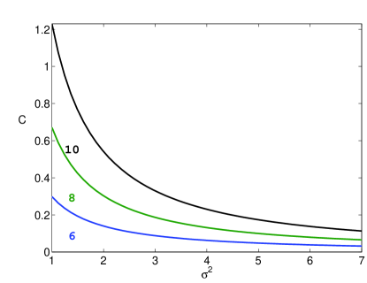
Figure 1: (Color online) Amplitude of the fluctuations $C$ for the exponential nonlocality versus $\sigma^{2}$, after Eq.(18), for various soliton powers $P$.

Figure 2: (a) Typical dynamics of a solitary wave [Eq.(3)] as obtained from the numerical solutions of the stochastic equation (4) in the presence of randomness and exponential nonlocality ($P=6$, $\sigma^{2}=5$, $\eta_{N}=0.01$); (b) Center of mass trajectories of the same bound-state ($P=6$, $\sigma^{2}=5$) for $100$ disorder realizations ($\eta_{N}=0.01$).

Figure 3: (Color online) Comparison of the numerically (continuous lines, $P=6$, $\eta_{N}=0.01$) and theoretically (circles for $\sigma^{2}=2$, squares for $\sigma^{2}=5$ and diamonds for $\sigma^{2}=10$) calculated standard deviation of the solitary wave position versus the evolution coordinate for three degrees of nonlocality and $100$ disorder realizations.

Before concluding, we consider the effect of non-paraxiality on the SW fluctuations. Ultra-thin nonlocal OSS were considered in Conti et al. (2004, 2005); in this framework, non-paraxiality at the lowest order is described by the perturbation $s=-\epsilon\psi_{xxxx}$,where $\epsilon$ is ratio between the wavelength and the spatial beam waist (within some numerical constants, see Conti et al. (2005)). Such a term is orthogonal to all the adjoint functions, with the exception of $\hat{f}_{\theta}$; this implies that Eq.(18) for the solitary-wave fluctuations still holds true in the ultra-focused regime, with the addition of a linear increase of the soliton phase along propagation:

$$\delta\theta_{\text{non-paraxial}}=-t\frac{2\epsilon}{P^{\prime}}\int u_{\beta}u_{xxxx}dx\text{,}$$ (21)

corresponding to the perturbation to the nonlinear wave-vector of the bound-state due to the non-paraxial term.

Conclusions — We have theoretically shown that nonlocality largely affects the dynamics of a solitary-wave in the presence of disorder; this turns out into a random walk of the self-trapped beam position, which is hampered by the filtering action of the nonlocal response, and ideally vanishes for a infinite degree of nonlocality. These results are expected to be specifically relevant for plasma-physics, Bose-Einstein condensates, thermal and thermo-diffusive media, liquid crystals and soft-colloidal matter, and suggest to employ highly nonlocal media for routing information by solitons in order to moderate the effect of randomness.

We acknowledge support from the CASPUR and CINECA High Performance Computing initiatives. The research leading to these results has received funding from the European Research Council under the European Community’s Seventh Framework Program (FP7/2007-2013)/ERC grant agreement n.201766.

References

- Kivshar and Agrawal (2003) Y. S. Kivshar and G. P. Agrawal, Optical solitons (Academic Press, New York, 2003).
- Whitham (1999) G. B. Whitham, Linear and Nonlinear Waves (Wiley, New York, 1999).
- Trillo and Torruealls (2001) S. Trillo and W. Torruealls, eds., Spatial Solitons (Springer-Verlag, Berlin, 2001).
- Snyder and Mitchell (1997) A. W. Snyder and D. J. Mitchell, Science 276, 1538 (1997).
- Conti et al. (2003) C. Conti, M. Peccianti, and G. Assanto, Phys. Rev. Lett. 91, 073901 (2003).
- Rotschild et al. (2005) C. Rotschild, O. Cohen, O. Manela, M. Segev, and T. Carmon, Phys. Rev. Lett. 95, 213904 (2005).
- Rasmussen et al. (2005) P. D. Rasmussen, O. Bang, and W. Królikowski, Phys. Rev. E 72, 066611 (2005).
- Buccoliero et al. (2007) D. Buccoliero, A. S. Desyatnikov, W. Krolikowski, and Y. S. Kivshar, Phys. Rev. Lett. 98, 053901 (2007).
- Kartashov and Torner (2007) Y. V. Kartashov and L. Torner, Opt. Lett. 32, 946 (2007).
- Ouyang and Guo (2009) S. Ouyang and Q. Guo, Opt. Express 17, 5170 (2009).
- Królikowski and Bang (2000) W. Królikowski and O. Bang, Phys. Rev. E 63, 016610 (2000).
- Segev et al. (1992) M. Segev, B. Crosignani, A. Yariv, and B. Fischer, Phys. Rev. Lett. 68, 923 (1992).
- Ghofraniha et al. (2007) N. Ghofraniha, C. Conti, G. Ruocco, and S. Trillo, Phys. Rev. Lett. 99, 043903 (2007).
- Conti et al. (2009) C. Conti, A. Fratalocchi, M. Peccianti, G. Ruocco, and S. Trillo, Phys. Rev. Lett. 102, 083902 (2009).
- Ghofraniha et al. (2009) N. Ghofraniha, C. Conti, G. Ruocco, and F. Zamponi, Phys. Rev. Lett. 102, 038303 (2009).
- Conti et al. (2005) C. Conti, G. Ruocco, and S. Trillo, Phys. Rev. Lett. 95, 183902 (2005).
- Parola et al. (1998) A. Parola, L. Salasnich, and L. Reatto, Phys. Rev. A 57, R3180 (1998).
- Perez-Garcia et al. (2000) V. M. Perez-Garcia, V. V. Konotop, and J. J. Garcia-Ripoll, Phys. Rev. E 62, 4300 (2000).
- Litvak and Sergeev (1978) A. G. Litvak and A. M. Sergeev, JETP Lett. 27, 517 (1978).
- Pecseli and Rasmussen (1980) H. L. Pecseli and J. J. Rasmussen, Plasma Phys. 22, 421 (1980).
- Peccianti et al. (2004) M. Peccianti, C. Conti, G. Assanto, A. De Luca, and C. Umeton, Nature 432, 733 (2004).
- Peccianti et al. (2002) M. Peccianti, C. Conti, G. Assanto, A. De Luca, and C. Umeton, Appl. Phys. Lett. 81, 3335 (2002).
- Skipetrov (2003) S. E. Skipetrov, Phys. Rev. E 67, 016601 (2003).
- Conti et al. (2007) C. Conti, L. Angelani, and G. Ruocco, Phys.Rev.A 75, 033812 (2007).
- Schwartz et al. (2007) T. Schwartz, G. Bartal, S. Fishman, and M. Segev, Nature 446, 52 (2007).
- Staliunas (2003) K. Staliunas, Phys. Rev. A 68, 013801 (2003).
- Sacha et al. (2009) K. Sacha, C. A. Müller, D. Delande, and J. Zakrzewski, Phys. Rev. Lett. 103, 210402 (2009).
- Fort et al. (2005) C. Fort, L. Fallani, V. Guarrera, J. E. Lye, M. Modugno, D. S. Wiersma, and M. Inguscio, Phys. Rev. Lett. 95, 170410 (2005).
- Kartashov et al. (2008) Y. V. Kartashov, V. A. Vysloukh, and L. Torner, Phys. Rev. A 77, 051802 (2008).
- Abdullaev and Garnier (2005) F. Abdullaev and J. Garnier, Progr. Opt. 48, 35 (2005).
- Conti (2005) C. Conti, Phys. Rev. E 72, 066620 (2005).
- Conti et al. (2006) C. Conti, N. Ghofraniha, G. Ruocco, and S. Trillo, Phys. Rev. Lett. 97, 123903 (2006).
- Sto (1999) Journ. of Low Temp. Physics 114, 11 (1999).
- Iannone et al. (1998) E. Iannone, F. Matera, A. Mecozzi, and M. Settembre, Nonlinear Optical Communication Networks (Wiley, New York, 1998).
- Gordon and Haus (1986) J. P. Gordon and H. A. Haus, Opt. Lett. 11, 665 (1986).
- Werner and Drummond (1997) M. J. Werner and P. D. Drummond, J. Comput. Phys. 132, 312 (1997).
- Qiang and Habib (2000) J. Qiang and S. Habib, Phys. Rev. E 62, 7430 (2000).
- Conti et al. (2004) C. Conti, M. Peccianti, and G. Assanto, Phys. Rev. Lett. 92, 113902 (2004).