On the new physics reach of the decay mode
Abstract:
We present a complete method to construct QCD-protected observables based on the exclusive 4-body -meson decay in the low dilepton mass region. The core of the method is the requirement that the constructed quantities should fulfil the symmetries of the angular distribution. We have identified all symmetries of the angular distribution in the limit of massless leptons and explore: a new non-trivial relation between the coefficients of the angular distribution, the possibility to fully solve the system for the amplitudes and the construction of non-trivial observables.
We also present a phenomenological analysis of the new physics sensitivity of angular observables in the decay based on QCD factorisation. We further analyse the -conserving observables, , and . They are practically free of theoretical uncertainties due to the soft form factors for the full range of dilepton masses rather than just at a single point as for . They also have a higher sensitivity to specific new physics scenarios compared to observables such as . Moreover, we critically examine the new physics reach of -violating observables via a complete error analysis due to scale dependences, form factors and corrections. We have developed an ensemble method to evaluate the error on observables from corrections. Finally, we explore the experimental prospects of -violating observables and find that they are rather limited. Indeed, the -conserving (averaged) observables (with ) will offer a better sensitivity to large phases and may be more suitable for experimental analysis.
MZ-TH/10-04
IC/HEP/2010-02
CERN-PH-TH/2010-032
1 Introduction
The LHC era is just beginning. Flavour physics will play an important complementary role to direct searches for the theory that lies beyond the standard model (SM). One central strategy in this period is to construct observables that are mostly sensitive to specific types of new physics (NP), in such a way that a deviation could immediately provide information on the type of NP required: isospin breaking NP, presence of right-handed currents, scalars, etc. It is essential to work in a bottom up approach in the direction of constructing a decision tree that help us to discern which features the NP model must incorporate and then try to match them into a group of models.
Few decays are able to provide such a wealth of information with different observables as , ranging from forward-backward asymmetries () and isospin asymmetries to a large number of angular observables. Each of these observables can provide information on the different types of NP mentioned above. First published results from BELLE [1] and BABAR [2] based on decays already demonstrate their feasibility.
In the early years of LHC running one will be restricted to those observables that may be extracted from the angular distribution using relatively simple analyses. A study of those observables relevant for the first few may be found in [3]. However, once enough statistics have been accumulated to perform a full angular analysis based on the full 4-body decay distribution of the , one has the freedom to design observables with reduced theoretical uncertainties and specific NP sensitivity.
In [4], it was proposed to construct observables that maximise the sensitivity to contributions driven by the electro-magnetic dipole operator , while, at the same time, minimising the dependence on the poorly known soft form factors. This led to the construction of the observable , based on the parallel and perpendicular spin amplitudes of the . The basic idea behind the construction of the observable was inspired by the zero point of when calculated as a function of the dilepton mass squared, . The zero point has attracted a lot of attention because of its cleanliness; only at that point one gets a complete cancellation at LO of the form factor dependence and its precise position may provide information on the fundamental theory that lies beyond the SM. For the soft form factor dependence cancels at LO, not only at one point, but in the full region thus providing much more experimental information. Moreover, the angular observable is highly sensitive to new right-handed currents driven by the operator [5], to which is blind.
Looking for the complete set of angular observables sensitive to right-handed currents, one is guided to the construction of the so-called and which include longitudinal spin amplitudes [6]. The observables (with ) use the spin amplitudes as the fundamental building block. This provides more freedom to disentangle the information on specific Wilson coefficients than just restricting oneself to use the coefficients of the angular distribution as it was recently done in [7]. For instance, , being directly proportional to enhances its sensitivity to the type of NP entering this coefficient. Moreover, using each coefficient of the angular distribution instead of selected ratios of them induces a larger sensitivity to the soft form factors.
The spin amplitudes are not directly observable quantities; to ensure that a quantity constructed out of the spin amplitudes can be observed, it is necessary that it fulfils the same symmetries as the angular distribution. This observation has the important consequence [6] that (first proposed in [8]) cannot be extracted from the angular distribution because it does not respect all its symmetries. Only a measurement of definite helicity distributions would allow it, but that is beyond any particle physics experiment that can currently be imagined [6].
To identify all the symmetries of the angular distribution is one of the main results of this paper. We discuss the counting of all the symmetries of the distribution in different scenarios, with and without scalars and with and without mass terms. We explain the general method of infinitesimal transformations that allow us to identify all the symmetries, and we develop here in full detail the explicit form of the four symmetries in the massless case with no scalars. As an important cross check of this result, we solve explicitly the set of spin amplitudes in terms of the coefficients of the distribution, making use of three out of the four symmetries. Two important consequences of this analysis are: in solving the system one naturally encounters an extra freedom to fix one of the variables, and there is a non-trivial constraint between the coefficients of the angular distribution considered before as free parameters. It is remarkable that this unexpected constraint is valid for any decay that has this same structure.
Finally, we provide an illustrative example of the use of the method of designing observables with an observable called that mixes simultaneously left/right and perpendicular/parallel spin amplitudes in a specific way that none of the coefficients of the angular distribution exhibits, opening different sensitivities to Wilson coefficients.
In the second part of the paper we present a phenomenological analysis of the various angular observables based on a QCD factorisation (QCDf) calculation to NLO precision. Recently, a very detailed analysis of angular quantities of the decay in various NP scenarios [7] and also an analysis of the NP sensitivities of angular asymmetries [9] were presented. In contrast to the former work [7], we do not assume that the main part of the corrections are inside the QCD form factors, but use the soft form factors and develop a new ensemble method for treating these unknown corrections in a systematic way. The main differences to the latter analysis of violating observables is the redefinition of the asymmetries in order to eliminate the soft form factor dependence at LO and the inclusion of the corrections into the error budget, which turn out to be significant in the presence of new weak phases.
In [6] the experimental preparations for an indirect NP search using these angular observables were worked out, showing that a full angular analysis of the decay at the LHCb experiment offers great opportunities. We re-evaluate this analysis in light of the fourth symmetry for the angular distribution and conclude that it has no effect on the estimated experimental errors as all observables are indeed invariant under this symmetry. We extend the experimental sensitivity study to -violating observables and show that even with an upgraded LHCb there is no real sensitivity to -violating NP phases in and .
The paper is organised as follows: Sec. 2 briefly recall the differential distribution in and the theoretical framework of QCDf and soft-collinear effective theory (SCET), Sec. 3 extends and completes our previous discussion about symmetries in the angular distribution, its experimental consequences are discussed in Sec. 4, and we perform a phenomenological analysis of the -violating and -conserving observables in Secs. 5 and 6 respectively.
2 Theoretical framework
The separation of NP effects and hadronic uncertainties is the key issue when using flavour observables in a NP search. Our analysis is based on QCDf and SCET and critically examines the NP reach of those observables via a detailed error analysis including the impact of the unknown corrections. In order to make the paper self contained, we briefly recall the various theoretical ingredients of our analysis.
2.1 Differential decay distribution
The decay , with on the mass shell, is completely described by four independent kinematic variables, the lepton-pair invariant mass squared, , and the three angles , , . Summing over the spins of the final state particles, the differential decay distribution of can be written as
| (1) |
The dependence on the three angles can be made more explicit:
| (2) |
As the signs of the expression depend on the exact definition of the angles, we have made their definition explicit in Appendix A.
The depend on products of the six complex spin amplitudes, , and in the case of the SM with massless leptons. Each of these is a function of . The amplitudes are just linear combinations of the well-known helicity amplitudes describing the transition:
| (3) |
Two generalisations will be made from the massless case within our analysis: if the leptons are considered massive the additional amplitude has to be introduced. And if we allow for scalar operators, there is a new amplitude . Both can be introduced independently of the other. For the we find the following expressions (see also [10, 11, 12, 4]) ***The generalizations to the case which includes scalar operators was recently presented in [7].:
| (4a) | ||||
| (4b) | ||||
| (4c) | ||||
| (4d) | ||||
| (4e) | ||||
| (4f) | ||||
| (4g) | ||||
| (4h) | ||||
| (4i) | ||||
| (4j) | ||||
| (4k) | ||||
| (4l) | ||||
with
| (5) |
The notations with the letters - has been included to make the comparison to [6] easier. Note that in the massless case.
The amplitudes themselves can be parametrised in terms of the seven form factors by means of a narrow-width approximation. They also depend on the short-distance Wilson coefficients corresponding to the various operators of the effective electroweak Hamiltonian. The precise definitions of the form factors and of the effective operators are given in [6]. Assuming only the three most important SM operators for this decay mode, namely , , and , and the chirally flipped ones, being numerically relevant, we have ††† Following common convention, we use the effective Wilson coefficients of these operators which include contributions from four-quark operators as well.
| (6a) | ||||
| (6b) | ||||
| (6c) | ||||
| (6d) | ||||
where the denote the corresponding Wilson coefficients and
| (7) |
| (8) |
Finally we note that, if one additionally considers scalar operators then is modified by the new Wilson coefficients and an additional amplitude, , proportional to the form factor , is introduced.
2.2 QCDf/SCET framework
The up-to-date predictions of exclusive modes are based on QCDf and its quantum field theoretical formulation, soft-collinear effective theory (SCET) [13, 14]. The crucial theoretical observation is that in the limit where the initial hadron is heavy and the final meson has a large energy [15] the hadronic form factors can be expanded in the small ratios and , where is the energy of the meson that picks up the quark from the decay. Neglecting corrections of order and , the seven a-priori independent form factors reduce to two universal form factors and [15, 16]. These relations can be strictly derived within the QCDf and SCET approach and lead to simple factorisation formula for the form factors
| (9) |
There is also a similar factorisation formula for the decay amplitudes. The rationale of such formulae is that the hard vertex renormalisations () and the hard scattering kernels () are quantities that can be computed perturbatively so they can be separated from the non-perturbative functions that go with them; i.e. the light-cone wave functions () which are process-independent and the soft form factors () which enter in several different processes.
In general we have no means to calculate corrections to the QCDf amplitudes so they are treated as unknown corrections, with the method used for this described in the following section. This, in general, leads to a large uncertainty of theoretical predictions based on the QCDf/SCET which we will explore systematically and make manifest in our phenomenological analysis.
We do not follow here the approach of [7] where the full QCD form factors are used in the QCDf formulae. There it is assumed that the main part of the corrections are inside the QCD form factors, and additional corrections are just neglected. Clearly some of the corrections could be moved into the full QCD form factors. However, there is no robust quantitative estimate of the additional corrections and, thus, it is not allowed to neglect those unknown corrections, especially in view of the expected smallness of new physics effects.
We follow here another strategy. We construct observables in which the soft form factor dependence cancels out at leading order. Then the influence of the soft form factors to the physics is almost eliminated from the phenomenological analysis in a controlled way. On the other hand we make the uncertainty due to corrections manifest in our analysis. It is not expected that there are as large as as in the decay as argued below. The inclusion of the errors due to the corrections in our analysis is exploratory of its impact on our observables, even at the risk to be too conservative. Obviously, it is this issue which calls for improvement in view of the new physics reach of these modes.
The theoretical simplifications of the QCDf/SCET approach are restricted to the kinematic region in which the energy of the is of the order of the heavy quark mass, i.e. . Moreover, the influences of very light resonances below 1 question the QCDf results in that region. In addition, the longitudinal amplitude in the QCDf/SCET approach generates a logarithmic divergence in the limit indicating problems in the theoretical description below 1 [13]. Thus, we will confine our analysis of all observables to the dilepton mass in the range, .
Using the discussed simplifications, the spin amplitudes at leading order in and have the very simple forms:
| (10a) | ||||
| (10b) | ||||
| (10c) | ||||
| (10d) | ||||
with , . Here we neglected terms of . The scalar spin amplitude is also proportional to in this limit.
2.3 Estimating corrections
Our observables have reduced theoretical uncertainties due to the cancellation of the soft form factors. However, the relations used to make these cancellations are only valid at LO in the expansion, and corrections to higher orders are unknown. For these theoretically clean observables to be useful, the impact of these corrections on the observables must be robustly bounded. If NP is to be discovered in , it must be possible to demonstrate that any effect seen is indeed NP and not just the effect of an unknown SM correction.
To evaluate the effect of the corrections, we parametrise each of the spin-amplitudes with some unknown linear correction,
| (11) |
where is the relative amplitude and the relative strong phase. If we vary and within their allowed ranges, an estimate for the theoretical uncertainty due to these unknown parameters can be found. In order to make this parametrisation generic, however, extra terms must be introduced. In principle the effective Hamiltonian which controls the decay has three terms,
| (12) |
The first term is very small as it is suppressed by the factor but is responsible for all the SM -violation in the decay; the second term is responsible for the decay in the SM; and the third adds possible NP contributions. A fourth possible term generically does not contribute to the model independent amplitudes and is neglected. Each of these contributions is generated by different sets of diagrams and may have different values of and .
Each amplitude must be modified to include the three sub-amplitudes with their corrections:
| (13) |
It is assumed that only a single NP operator is active so as not to introduce extra terms. In this formalism, the SM -violating, SM -conserving, and NP parts of the amplitude are then allowed to have independent corrections and strong phases.
An estimate of the theoretical uncertainty arising from the unknown corrections and strong phases can now be made using a randomly selected ensemble. For each member of the ensemble, values of and are chosen in the ranges or and from a random uniform distribution. This is done for the seven amplitudes, , , , , to provide a complete description of the decay. It is assumed that the corrections and phases are not functions of , although in practise they may actually be. Any unknown correlations are also ignored. While these effects could lead to an underestimate of the theoretical envelope, it is thought that this method allows for a conservative estimate of the theoretical uncertainties to be made.
To estimate the contribution to the theoretical uncertainties from corrections for a particular observable, each element in the ensemble was used to calculate the value of that observable at a fixed value of . A one error is evaluated as the interval that contains 66% of the values around the median. This is done for both and to illustrate the effects of five and ten percent corrections. By repeating this process for different values of , bands can be built up. No assumption of Gaussian statistics has been made; the bands illustrate the probable range for the true value of each observable, given the current central value. The method allows for the probability that a given experimental result is due to an unknown SM correction to be found.
The choice is based on a simple dimensional estimate. We emphasize here that there is no strict argument available to bound the corrections this way. But we can state that the chiral enhancement of corrections in the case of hadronic decays does not happen in the case of the semileptonic decay mode with a vector final state.
The process described here avoids any assumptions about correlations between the corrections and is thus statistically more rigorous than what was done in [6], where corrections to amplitudes were considered one by one and then added in quadrature. The bands it produces are reduced when compared to those of [6]. It also allows us to investigate the effect of the corrections for -violating observables.
3 Symmetries and observables
The experimental degrees of freedom determined by the terms and the theoretical degrees of freedom determined by the spin amplitudes have to match. There are two effects to consider for this: different values of the can give rise to the same differential distribution Eq. (1) and thus cannot be distinguished; and in some cases the experimental coefficients are not independent, meaning that not all arbitrary values of the are possible. The first effect we call a continuous symmetry transformation. For the degrees of freedom to match we have
| (14) |
where is the number of coefficients in the differential distribution (the number of ), the number of dependencies between the different coefficients, the number of spin amplitudes (the , each is complex and hence has two degrees of freedom), and the number of continuous symmetries.
We considered this situation in our previous paper [6] for the case of massless leptons and return to it again here. It is easy to see that in the massless limit, and . What is not so obvious is that can be expressed in terms of the other 8 remaining coefficients. Going back to Eq. (14) it can be seen that the massless case in fact must have 4 symmetries and not 3 as we claimed in the previous paper.
Below we first outline how the symmetries and dependencies can be identified before we move onto their explicit form and the interpretation.
3.1 Infinitesimal symmetries
By an infinitesimal symmetry is meant one where the theoretical spin amplitudes are changed in an infinitesimal way leaving the coefficients in Eq. (4) unchanged. The infinitesimal symmetries will define a system of coupled ordinary differential equations that, if solved, are the global symmetries we look for. There is no guarantee that these symmetries will allow for the continuous transformation between two arbitrary sets of amplitudes which have the identical angular distribution; there could in principle be several disjoint regions separated by divergences.
If we, in this example, look at massless leptons and ignore the scalar amplitude, the coefficients of the spin amplitudes can be defined as a vector with 12 components
| (15) | |||||
corresponding to the real and imaginary parts of the amplitudes. For each of the coefficients we can find the derivative with respect to the spin amplitudes. As an example
| (16) |
There will be eleven such gradient vectors in the massless case, as .
Now, any infinitesimal transformation can be written on the form
| (17) |
For the infinitesimal transformation to leave the coefficients unchanged, the vector has to be perpendicular to the hyperplane spanned by the set of gradient vectors. Or in other words, represents a symmetry if, and only if
| (18) |
Looking back at Eq. (14) we have, for the massless case, . If the were all independent the gradient vectors would span an 11 dimensional hyperplane. In fact, it turns out that they only span 8 dimensions‡‡‡Any program able to handle symbolic algebra will be able to show this., which shows that there are three dependencies between the ’s, giving . As we have from the amplitudes we see from Eq. (14) that we have corresponding to 4 symmetries. For the dependencies, only the first two and are trivial; the third one we derive in the next section.
3.2 Explicit form of symmetries
It is helpful for the discussion to make the following definitions.
| (19a) | ||||
| (19b) | ||||
| (19c) | ||||
or in terms of helicity amplitudes
| (20a) | ||||
| (20b) | ||||
| (20c) | ||||
In fact, all the information of the angular distribution is encoded in the moduli of the three vectors and their relative complex scalar products:
| (21) | |||||
| (22) |
where being a complex vector implies that the scalar product is . The coefficients and are absent because they are obviously redundant.
The differential distribution is invariant under the following four independent symmetry transformations of the amplitudes
| (23) |
where , , and can be varied independently. Identical transformations can be carried out on the . Normally, there is the freedom to pick a single global phase, but as and amplitudes do not interfere here, two phases can be chosen arbitrarily as reflected in the first transformation matrix.
The interpretation of the third and fourth symmetry is that they transform a helicity final state with a left handed current into a helicity state with a right handed current. As we experimentally cannot measure the simultaneous change of helicity and handedness of the current, these transformations turn into symmetries for the differential decay rate.
3.3 Relationship between coefficients in differential distribution
As was mentioned earlier, we have identified an extra dependency among the coefficients in the massless case. Here we outline how it can be derived.
If we use the two global phase symmetry transformations we can rotate the vector to make it real ( and become real).§§§Indeed the system can also be solved using only one of the two global symmetries and keep complex. We can then choose the angle of the third symmetry to make . Notice that we have not made use of the fourth symmetry. The implications of this fourth symmetry will become manifest when solving the system. With these choices
| (24) |
where is a positive real parameter. Using three of Eqs. (21)-(22) together with the symmetries, one can determine four of the spin amplitudes (their moduli and phases):
| (25a) | ||||
| (25b) | ||||
| (25c) | ||||
| (25d) | ||||
The remaining three equations from Eqs. (21)-(22) determine, on one side, the moduli of and ,
| (26a) | ||||
| (26b) | ||||
and on the other, the phase difference corresponding to the previous two amplitudes:
| (27) |
Here is where the fourth symmetry becomes manifest. On one side, this equation tells us that you have the freedom to choose one of the two phases or to zero. On the other side, given that the LHS of the previous equation is a pure phase, the modulus of the RHS should be one. This implies the following important non-trivial relationship between the coefficients of the distribution
| (28) |
It is important to remark that this equation can be very easily generalised to the massless case with scalars using the relations and in the previous equation. Also the massive case with no scalars can be included by introducing the factors inside the coefficients. There is no such equation in the massive case with scalars due the fact that the number of coefficients of the experimental distribution is identical to the number of theoretical amplitudes and symmetries (see Tab. 1).
3.4 Experimental issues
The symmetries discussed above can be used to fix the spin-amplitude components by choosing specific values of the relevant rotation angles. We give an explicit example of this for the case where the lepton mass is neglected. We choose to make the following constraint:
| (29) |
This can be achieved by first performing the last transformation, shown in Eq. (23), with the value of given by:
| (30) | ||||
| where | ||||
| (31) | ||||
Next, the third rotation angle, , is used again in Eq. (23):
| (32) |
The -fields are phase-shifted by :
| (33) |
and finally the last -field transformation can be performed substituting and into the previous expression:
| (34) |
3.5 Constructing observables
In [4, 6], as well as here, we use the spin amplitudes to construct our observables. There are two main advantages of this approach, one is experimental and the other is theoretical. On the experimental side, we have found that fitting directly the angular coefficients , without taking into account the relations between them, leads to fit instabilities. These relations, coming from the underlying spin amplitudes, can be found in Sec. 3.3. The theoretical argument has to do with our aim at constructing observables that fulfil certain criteria, namely maximal sensitivity to a specific NP operator, like new right-handed currents, and minimal sensitivity to poorly known form factors. Given that our main tools are the spin amplitudes, it is a straight-forward exercise to design observables with a specific NP sensitivity and small hadronic uncertainties. We also have more freedom to construct observables than just using each coefficient of the distribution as an observable. As the spin amplitudes can be extracted directly in the full-angular analysis, there is no penalty on the final experimental uncertainty from using a non-trivial functional form to make the observable.
The symmetries of the angular distribution play a crucial role in our approach. Once a quantity has been designed, it is a necessary condition for being an observable based on the angular distribution that it respects all the symmetries of this distribution. For example in [6], we have shown explicitly that a previously discussed transversity amplitude does not fulfil all the symmetries of the angular distribution. This implies that this quantity cannot be measured at the LHCb experiment or at future super- factory experiments; a measurement of the spins of the final-state particles would be required for that.
Let us finally discuss a new -conserving observable that we call . It is defined as:
| (35) |
It probes the transverse spin amplitudes and in a different way than . Direct inspection of Eq. (4) shows that there is no single angular coefficient mixing with and with simultaneously in the way does.
It is a simple exercise to check that this observable fulfils the four symmetries described in Eq. (23). Once this invariance is fulfilled¶¶¶Notice one could try to write in terms of the using the explicit solution, but this is not allowed since is not invariant [6]. one is allowed to use the explicit solution in the massless case provided in the previous subsection Eqs. (21)-(22):
| (36) |
A discussion on the properties and sensitivities of this observable is presented in Sec. 6.
3.6 More general cases
The discussion of the differential symmetries from Sec. 3.1 can be generalised to the cases where the leptons are no longer considered massless and where a scalar amplitude is included:
- Massless leptons with scalars
-
The inclusion of the scalar amplitude , gives us seven amplitudes. The four explicit symmetries in Eq. (23) are still valid and we have in addition
(37) expressing that the phase of cannot be determined.
- Massive leptons without scalars
-
We have the seven amplitudes , , and in this case and still eleven coefficients. As a fact of elementary quantum mechanics we still have a global phase transformation corresponding to , but the other two symmetries from the massless case are no longer valid. There is a new symmetry concerning the phase of given as:
(38) This leaves us with two symmetries where only the differential form is known.
- Massive leptons with scalars
-
We now have all eight amplitudes and, with the inclusion of , we have twelve coefficients. The global phase transformation, , and the phase transformation of in Eq. (38) are still valid. In this case, there is no dependency between any of the coefficients, leaving us with two symmetries where only the differential form is known.
So while we in some cases only know the differential form of the symmetries, we are still able to test if observables respect the symmetries (see Sec 3.5) and we can also determine the optimal set of amplitudes to fit for in an experimental fit (see Sec. 3.4). In Tab. 1 we summarise the full knowledge about the symmetries.
| Case | Coefficients | Dependencies | Amplitudes | Symmetries |
|---|---|---|---|---|
| , | 11 | 3 | 6 | 4 |
| 11 | 2 | 7 | 5 | |
| , | 11 | 1 | 7 | 4 |
| 12 | 0 | 8 | 4 |
4 Experimental Sensitivities
In [6], a fitting technique was investigated that allowed the extraction of the spin amplitudes from the full angular distribution in the massless lepton limit. Eq. (1) can be interpreted as a probability density function (PDF) and normalised numerically. We parametrise it in terms of six complex spin amplitudes, which are functions of only. In the limit of infinite experimental data, and for a fixed value of , these amplitudes can be found by fitting the relative contribution of each angular coefficient as a function of the three decay angles. As discussed in Sec. 3, the symmetries of the distribution can then be used to reduce the number of unknowns; if we consider the real and imaginary amplitude components separately, the twelve parameters can be reduced to eight using the symmetry constraints. A further spin-amplitude component may be removed by noting that Eq. (1) is only sensitive to relative normalisations. This leaves seven free parameters at each point in . However, in [6], only three, out of four, symmetry constraints were considered meaning that, in principle, the fits presented were under-constrained. The implications of this will be investigated in this section.
Despite the large increases in statistics expected at LHCb, the number of signal events available will still be too small for a fixed approach to be taken. Instead, the spin-amplitude components are parametrised as second-order polynomials in the region . These are normalised relative to the value of at a fixed value, , of . Rather than fitting directly for the amplitudes, we aim to extract the coefficients of these polynomials. This introduces a number of model biases: the underlying spin amplitudes are assumed to the smoothly varying in the window considered. As noted in [6], this was verified for a number of NP models. There is also an implicit assumption that the -dependent shape of the spin amplitudes is invariant under the symmetries of the angular distribution. Neglecting background parameters, the -dependent fit has free parameters to be extracted, or 26 in [6]. These will be labelled the four- and three-symmetry fits respectively.
The three-symmetry fit although, in principle, under-constrained is able to converge due to the polynomial parametrisation employed. By requiring that three of the spin amplitude components vanish for all values of , we have used our freedom to choose values of , , and from Eq. (23) at each point in ; the value of is still free to vary. However, the PDF, Eq. (1), is invariant under changes of ; hence, the negative log-likelihood (NLL) used during minimisation should not be sensitive to its value. The dependent shape of each amplitude component is manifestly not invariant under changes in – the rotation it implies mixes the imaginary parts of the left- and right-handed amplitudes. The polynomial parametrisation of the spin-amplitude components requires that each amplitude must be smoothly varying. The fit then selects the value of for each signal event which produces the most polynomial-like distribution, as this will have the smallest NLL. The general minimising algorithm employed is then able to find a genuine minimum and converge properly; the imposition of the polynomial ansatz allowed the under-constrained fit of [6] to converge properly. As the experimental observables are invariant under all four symmetries, their dependent distributions can be found correctly; there are no significant biases seen in the central values extracted compared to the input distribution. Small biases are seen in the individual spin-amplitude components; with hindsight, correlations between these components were induced by the presence of the fourth symmetry.
4.1 Experimental Analysis
The discussion above explains why the three-symmetry fit is able to converge successfully, and suggests that there should be no change in the experimental uncertainties found when the extra symmetry constraint is added. It is important to demonstrate that this is the case. As before, the experimental sensitivity to different observables can be estimated using a toy Monte Carlo (MC) approach and used to compare the three- and four-symmetry fits.
4.1.1 Generation
An ensemble of data sets for can be generated; each data set contains the Poisson fluctuated number of signal and background events expected after LHCb has collected 10 of integrated luminosity. Estimates of the signal and background yields were taken from [17, 18] and scaled linearly. The signal distribution was generated using the spin amplitudes discussed in Sec. 2 as input. The contribution from terms including the muon mass were included. No assumption of polynomial variation of the amplitudes was used in the generation. The signal is assumed to have a Gaussian distribution in with a width of in a window of and a Breit-Wigner in with width in a window of . A simplified background model is included; it is flat in all decay angles, effectively treating all background as combinatorial, but follows the distribution of the signal. Detector acceptance effects as described in [17] are not taken into account. When considering -conserving quantities, the and samples are simply considered together. We do not include any contributions from non-resonant .
4.1.2 Observable sensitivities
The ensemble of simulated data sets can then be used to estimate the experimental uncertainties expected for a given integrated luminosity at LHCb. For each data set, the full angular fit was performed to find the most likely value for each of the free parameters for that data set. For the three-symmetry fit there were 27 free parameters; 26 for the signal distribution and one to describe the level of background seen. For the four-symmetry fit, only 24 parameters were required. In total we created an ensemble of 1200 experiments and will, thus, at a given value of , get 1200 different determinations of each observable. By looking at the point where 33% and 47.5% of results lie within either side of the median of the results we can form asymmetric and errors. Connecting these at different values gives us and bands for the experimental errors on the observable.
4.1.3 asymmetries
The sensitivity to various asymmetries was also considered. In this case, separate and samples were generated and fit independently. Each sample had on average half the number of signal and background events as those described in Sec. 4.1.1. The results of a and a fit could then be combined by re-normalising the amplitudes found, so that the extracted value of at was the same in both samples. This gives sensitivity to asymmetries relative to this point. By considering many and samples together, estimates of the experimental sensitivity to the asymmetries could then be found. In a real measurement, a more sophisticated approach would be taken which considered the two samples simultaneously; however, our simplified approach gives a reasonable first estimate of the experimental sensitivities obtainable and allow comparison with theoretical requirements.
4.2 The polynomial ansatz re-examined
A key assumption of the fitting approach taken in [6] is that the spin-amplitude components are smoothly varying functions in the range . It was found that when all four symmetries of the massless angular distribution are taken into account, this assumption no longer holds; indeed the shape of the spin-amplitude components is not invariant under the four symmetries and their shape can be distorted so they are no longer well described by second-order polynomials. Other parameterization choices are likely to be equally vulnerable to these problems unless they are explicitly invariant under all symmetries of the angular distribution. Consider the three-symmetry case at a fixed value: in [6], is removed by setting once their phases have been rotated away. This can be understood by substituting the trigonometric identities,
| (39) |
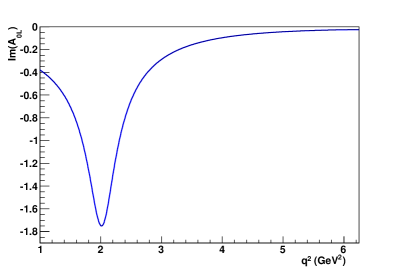
into Eq. (23). This introduces a term into each non-zero amplitude component, which will not be well behaved as . For the three-symmetry fit, these problems can be avoided by taking as the reference amplitude component, forcing it to be relatively large at . However, to include the fourth symmetry constraint, a more complicated form must be used in order to set four amplitude components simultaneously. A different value of each of the four rotation angles is required for every point in due to the changing spin amplitudes. There is no guarantee that a set of rotation angles can be found such that the unfixed spin-amplitude components resemble smoothly varying polynomials for all . The dependence of the SM input amplitude is shown in Fig. 1 once the four symmetries have been applied to fix , , , and to zero, as required for in the next section. This particular feature is caused by at ; other rotation choices lead to similar features. The distribution can no longer be well described by a second-order polynomial. It may be possible to find a choice of rotation parameters that preserve the polynomial features of the input spin-amplitude components, however, there are no guarantee that a particular choice would work when faced with experimental data. Indeed, an incorrect choice will lead to biases in the case where the parametrisation is a poor match for the underlying amplitudes. A more generic solution is required and could form the basis for further investigations.
4.3 Fit Quality
The effect of adding the fourth symmetry constraint was tested, by comparing ensembles of three- and four-symmetry fits. The two ensembles were generated with the same random seed values so that the ensemble of input data sets was the same for the two approaches. The fixed spin-amplitude components were chosen to be , , , and in the case of the four-symmetry fit also . The amplitudes were still normalised relative to at , however the fits were performed in the range to avoid the non-polynomial features seen in the spin-amplitude components, such as shown in Fig. 1.
The sensitivities found for the angular observables are poorer than those presented in [6], due to the decreased signal statistics in the reduced window, however, it is interesting to compare the performance of the two fitting methods. A histogram of the NLL of each fit is shown in Fig. 3. The ensemble of three-symmetry fits (hatched) and four-symmetry fits (solid) can be seen. The ensemble of input data sets is slightly different in each case due to a small number of failed computing jobs, but the output distributions look very similar. This shows that the depth of the minima found is approximately the same for the three- and four-symmetry fits. We can also introduce a global correlation factor , which is the unsigned mean of the individual global correlation coefficients calculated from the full covariance matrix. It takes values in the range , where zero shows all variables as completely uncorrelated, and one shows total fit correlation. It can be seen in Fig. 3 that the mean correlation of the fit is reduced once the fourth symmetry is taken into account. There are less outliers at very low and the distribution appears more Gaussian, indicating an increase in fit stability has been achieved. The convergence of the fit starting from arbitrary initial parameters has also much improved.
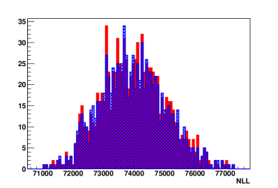
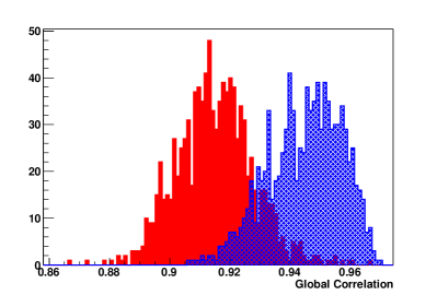
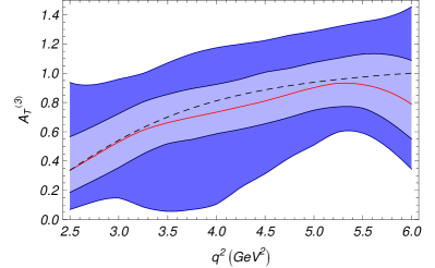
Fig. 4 shows the estimated experimental sensitivities found for the theoretically clean observable in the range , with and without the fourth symmetry constraint. The fits are for 10 of LHCb integrated luminosity assuming the SM. As might be expected from Fig. 3, there is little difference in the estimated experimental resolutions seen. The same conclusion is reached when inspecting other observables.
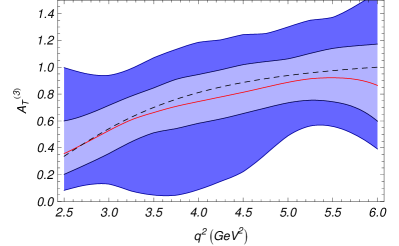
4.4 Discussion
The discovery of a fourth symmetry in the massless leptons limit of the full-angular distribution of requires that the experimental analysis proposed in [6] be re-evaluated. The previous analysis used three of the four available symmetry constraints to perform a fit, that was, in principle, under-constrained, by parametrising the real and imaginary parts of the spin amplitudes as second-order polynomials. The invariance of the observables under all four symmetries, and the freedom to take arbitrary values of the rotation angle, allowed the fits to converge and produce correct output, but introduced a subtle parametrisation bias. As the observables are by definition invariant to all the symmetries, the estimated experimental sensitivities are the same for the two methods. This has been demonstrated in this section. However, the need for the development of a new fitting method, so that the full experimental statistics available in can be used, is now clear. The sensitivities found will be similar to those estimated in Ref. [6] and in this paper for the asymmetries, but with improved fit stability.
5 Analysis of -violating observables
In [10, 19], it was shown that eight -violating observables can be constructed by combining the differential decay rates of and . In this section we analyse the theoretical and experimental uncertainties of those observables in order to judge the NP sensitivity of such -violating observables.
5.1 Preliminaries
The corresponding decay rate for the -conjugated decay mode is given by
| (40) |
As shown in [10], the corresponding functions are connected to functions in the following way:
| (41) |
where equals with all weak phases conjugated.
Besides the asymmetry in the dilepton mass distribution, there are several -violating observables in the angular distribution. The latter are sensitive to -violating effects as differences between the angular coefficient functions, . As was discussed in [10, 19], and more recently in [9], those asymmetries are all very small in the SM; they originate from the small -violating imaginary part of . This weak phase present in the Wilson coefficient is doubly-Cabibbo suppressed and further suppressed by the ratio of the Wilson coefficients .
Moreover, it is important to note [19, 9] that the asymmetries corresponding to are odd under the transformation and thus, these asymmetries are T-odd (T transformation reverses all particle momenta and particle spins) while the other angular asymmetries are T-even. T-odd asymmetries are favoured because they involve the combination of the strong and weak phase differences [19, 9], thus, they are still large in spite of small strong phases as predicted for example within the QCDF/SCET approach. In contrast, T-even asymmetries involve the combination [19, 9]∥∥∥We note here that this specific behaviour of T-odd and T-even observables was shown in many examples of T-odd asymmetries (see [20] and references therein) but a general proof of this statement is still missing to our knowledge..
Another remark is that the asymmetries related to can be extracted from due to the property Eq. (41), and thus can be determined for an untagged equal mixture of and mesons. This is important for the decay modes and but it is less relevant for the self-tagging mode .
Recently, a QCDf/SCET analysis of the angular -violating observables, based on the NLO results in [13, 14], was presented for the first time [9]. The NLO corrections are shown to be sizable. The crucial impact of the NLO analysis is that the scale dependence gets reduced to the level for most of the asymmetries. However, for some of them, which essentially start with a nontrivial NLO contribution, there is a significantly larger scale dependence. The -integrated SM predictions are all shown to be below the level due to the small weak phase as mentioned above. The uncertainties due to the form factors, the scale dependence, and the uncertainty due to CKM parameters are identified as the main sources of SM errors [9].
5.2 Phenomenological analysis
The NP sensitivity of -violating observables in the mode was discussed in a model-independent way [9] and also in various popular concrete NP models [7]. It was found that the NP contributions to the phases of the Wilson coefficients , , and and of their chiral counterparts drastically enhance such -violating observables, while presently most of those phases are very weakly constrained. It was claimed that these observables offer clean signals of NP contributions.
However, the NP reach of such observables can only be judged with a complete analysis of the theoretical and experimental uncertainties. To the very detailed analyses in [9, 7] we add the following points:
-
•
We redefine the various asymmetries following the general method presented in our previous paper [6]: an appropriate normalisation of the asymmetries almost eliminates any uncertainties due to the soft form factors which is one of the major sources of errors in the SM prediction.
-
•
We explore the effect of the possible corrections and make the uncertainty due to those unknown corrections manifest in our analysis within the SM and NP scenarios.
-
•
We investigate the experimental sensitivity of the angular asymmetries using a toy Monte Carlo model and estimate the statistical uncertainty of the observables with statistics corresponding to five years of nominal running at LHCb () using a full angular fit method.
We discuss these issues by example of the two angular asymmetries corresponding to the angular coefficient functions and ;
| (42) |
Within the SM the first asymmetry related to turns out to be the well-known forward-backward asymmetry which was proposed in [21, 22].
As a first step we redefine the two observables. We make sure that the form factor dependence cancels out at the LO level by using an appropriate normalisation:
| (43) |
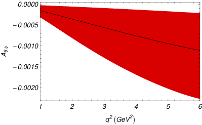
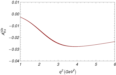

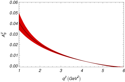
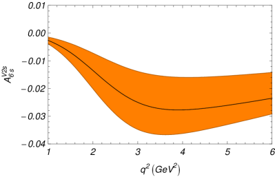
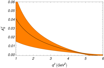
The are bilinear in the spin amplitudes, so it is clear from the LO formulae Eq. (6) that, following the strategy of [6], any form factor dependence at this order cancels out in both observables. We note that has the same form factor dependence as but has larger absolute values over the dilepton mass spectrum that stabilises the quantity. In Fig. 5 the uncertainty due to the form factor dependence is estimated in a conservative way (see Appendix B) for defined in Eq. (42) and for defined in Eq. (43). Comparing the plots, one sees that with the appropriate normalisation, this main source of hadronic uncertainties gets almost eliminated. The leftover uncertainty enters through the form factor dependence of the NLO contribution. Fig. 6 shows the analogous results for the observable .
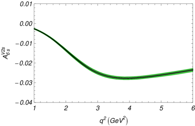
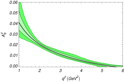
In the second step we make the possible corrections manifest in our final results by using the procedure described in Sec. 2.3. It turns out that in spite of this very conservative ansatz for the possible power corrections (we neglect for example any kind of correlations between such corrections in the various spin amplitudes), the impact of those corrections is smaller than the SM uncertainty in case of the two observables and . In the left plot of Fig. 7 the SM error is given, including uncertainties due to the scale dependence and input parameters and the spurious error due to the form factors. In the right plot the estimated power corrections are given, which in case of the -violating observable are significantly smaller than the combined uncertainty due to scale and input parameters. Fig. 8 shows the same feature for the -violating observable . This result is in contrast to the one for -averaged angular observables discussed in [6], where the estimated power corrections always represent the dominant error. The reason for this specific feature is the smallness of the weak phase in the SM. Thus, one expects that the impact of power corrections will be significantly larger when NP scenarios with new phases are considered (see below).
In the third step we consider various NP scenarios. Here we follow the model-independent constraints derived in [9] assuming only one NP Wilson coefficient being nonzero. We consider three different NP benchmarks scenarios of this kind:
-
1.
and (Red);
-
2.
and (Grey);
-
3.
and (Blue);
where the colours refer to the ones used in the following figures. The absolute values of the Wilson coefficients are chosen in such a way that the model-independent analysis, assuming one nontrivial NP Wilson coefficient acting at a time, does not give any bound on the corresponding NP phase.
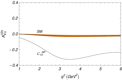
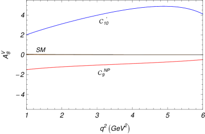
Fig. 9 shows our two observables in the three scenarios with the phase value : the -violating observable might separate a NP scenario (2), while the central values of scenarios (1) and (3) are very close to the SM. Moreover observable seems to be suited to separate scenarios (1) and (3) from the SM.
However, to judge the NP reach we need a complete error analysis within the three NP scenarios. As shown in Sec. 2.3 we now work with three weak sub-amplitudes in which possible power corrections are varied independently. The plots in Figs. 10 and 11 show that the possible corrections have a much larger impact on our two observables in the NP scenarios than in the SM and become the dominating theoretical uncertainty. We also get significantly larger possible corrections when changing the value of the new weak phase from to . Regarding even larger phase values, we note here that the NP effects drastically decrease again when phase values around are chosen as expected. Nevertheless, in view of the theoretical uncertainties only, the two -violating observables could discriminate some specific NP scenarios with new phase of order or from the SM; in case of NP scenario 2, in case of NP scenario 3 and possibly 1.
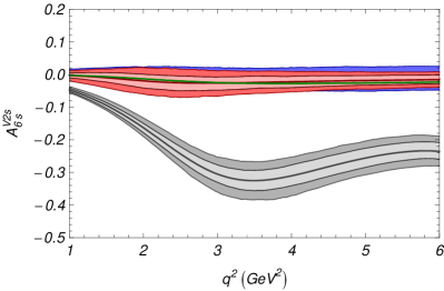
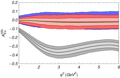
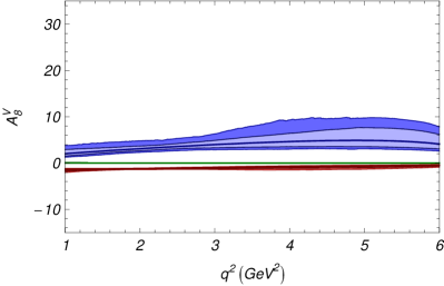
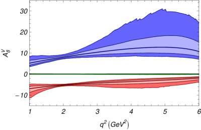
One should also consider the additional theoretical uncertainties due to scale dependence, input parameters and soft form factor dependencies within the NP scenarios. Those additional theoretical uncertainties are sizable and of the same order as the ones due to corrections: they are shown in the left plots in Figs. 12 and 13 as orange bands overlaying the total errors bars including also the corrections.
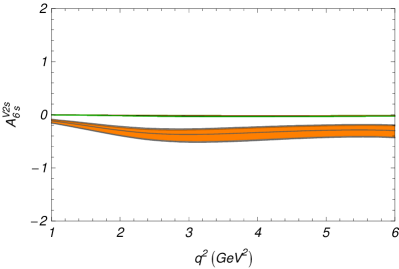
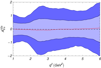
As the last step, we analyse the experimental sensitivity of the angular asymmetries using a toy Monte Carlo model. The right plots in Figs. 12 and 13 show the estimates of the statistical uncertainty of and with statistics corresponding to five years of nominal running at LHCb (). The inner and outer bands correspond to and statistical errors. The plots show that all the NP benchmarks are within the range of the expected experimental error in case of the observable , and within the range of the experimental error in case of the observable . We emphasise that from the experimental point of view the normalisation is not important when calculating the overall significance because the overall error is dominated by the error on the numerator. So the experimental error of the observables and defined in Eq. (42) using the traditional normalisation will be similarly large to the one of our new observables and defined in Eq. (43).
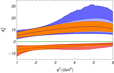
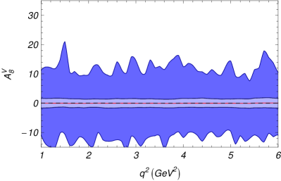
Our final conclusion is that the possibility to disentangle different NP scenarios for the -violating observables remains rather difficult. For the rare decay , LHCb has no real sensitivity for NP phases up to values of (and neither up to values of ) in the Wilson coefficients , and their chiral counterparts. Even Super-LHCb with integrated luminosity does not improve the situation significantly. This is in contrast to the -conserving observables presented in [6] and further discussed in the next chapter which, both from the theoretical and experimental point of view, are very promising.
6 Analysis of -conserving observables
The -conserving observables can be analysed at LO in the large recoil limit using the heavy-quark and large- expressions for the spin amplitudes, as first proposed in [4]. One of the advantages of this approach is that we obtain analytic expressions of these observables in a very simple way. These expressions can be used to study the behaviour of the observables without having to rely on numerical computations, since the most relevant features arise already at LO. The main goal of this section is to perform this type of analysis on the observables.
6.1 Leading-order expressions of
The asymmetry , first proposed in [4] is given by
| (44) |
where . It has a simple form, free from form factor dependencies, in the heavy-quark () and large energy () limits******Notice that along this section we will drop the superscript “eff” that and should bear in order to simplify the notation.:
| (45) |
where . The Wilson coefficients can take the most general form:
| (46) |
We will neglect henceforward both the tiny SM weak phase , that arises from the CKM elements ratio , and the SM strong phase , smaller than in the low dilepton mass region [22].
Obviously, the observable vanishes in the heavy-quark and large energy limits at LO when all the Wilson coefficients are taken to be SM-like. This result can be understood rather easily. The left-handed structure of weak interactions in the SM guarantees that, in these limits, the quark created in the transition will have helicity in the massless limit () [23]. This quark will combine with the spectator quark of the to form the meson with or (but not ), therefore at quark level in the SM. Using Eq. (3), this translates into at the quark level, which corresponds to at the hadron level [24, 25, 26].
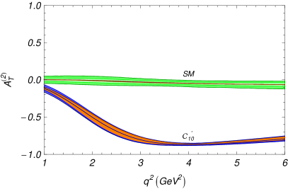
The NP dependence of can be studied in a model independent way by switching on one Wilson coefficient each time and keeping all the others at their SM values. A simple inspection of Eq. (45) shows that only the chirally flipped operators and give a non-zero expression for in our approximation:
| (47) |
and
| (48) |
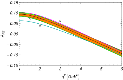
Equations. (48) and (47) show that is sensitive to both the modulus and the sign of the Wilson coefficients and . When NP enters only , the fact that in the SM makes the observable negative unless , enabling us to distinguish the sign of this weak phase (Fig. 14). Likewise, if NP appears in , will display a zero in the dilepton mass spectrum when , which will coincide exactly with the zero of the observable at LO [13]. As the zero is independent of , all curves with should exhibit it at , but if there is also a NP contribution to , the zero will be shifted either to higher or lower values of . In case of a sign flip affecting , would not have a zero at any value of , exactly as for (see [27] for a recent discussion of different mechanisms to achieve this). In fact, should NP enter both and simultaneously, Eq. (45) would imply
| (49) |
while
| (50) |
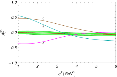
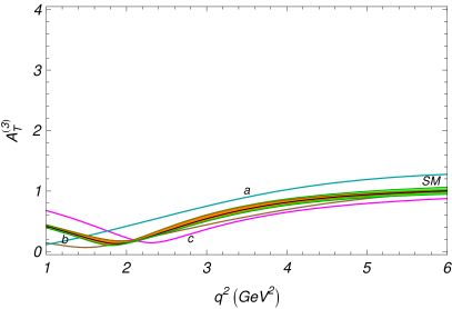
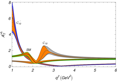
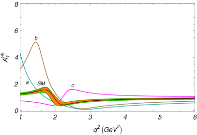
The comparison of Eq. (49) with Eq. (50) can be used to explain the improved sensitivity of to certain types of NP versus that of . The numerator of exhibits sensitivity to the weak phases and , having an interference term enhanced by the large factor ( in the dilepton mass region studied), while is only sensitive to . Thus, a wider departure from the SM behaviour is to be expected in when NP enters the operators and . This is shown in Fig. 15 using three different scenarios, described in the caption of Fig. 15, compatible with present experimental and theoretical constraints. Therefore, we emphasise that must be regarded as an improved version of once the full-angular analysis becomes possible.
6.2 Leading-order expressions of
In the SM, we get in the heavy-quark and large- limits at LO:
| (51) |
which sets the “wave-like” behaviour of . At low , Eq. (51) can be used to check that . On the other hand, at the zero-point of and , exhibits an absolute maximum of magnitude .
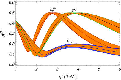
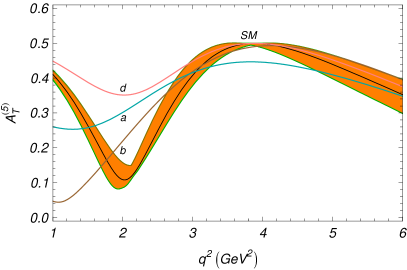
Any inclusion of NP in the Wilson coefficients , and will give rise to the appearance of an extra term in the numerator (with respect to Eq. (51)) that will shift the observable along the -axis.
| (52a) | ||||
| (52b) | ||||
| (52c) | ||||
In Eq. (52) we have chosen for simplicity the weak phase for , but they turn out to be dominated by the SM contribution unless the NP Wilson coefficients are very large. However, if the weak phases associated to NP Wilson coefficients are different from , the curve will get shifted either to the left or to the right, depending on the value of the angle, as shown in Fig. 16.
NP might also enter via the chirally flipped and . The corresponding LO expressions of in the heavy-quark and high- limits read
| (53) |
and
| (54) |
Equations (53) and (54) are both free from NP weak-phase dependence. evaluated at the value of the zero-point can be computed easily using Eq. (54), obtaining
| (55) |
where the choice enables us to recover the SM prediction . In Fig. 16 (left) it can be seen that for the departure of the NP curve obtained from the SM behaviour is indeed large.
6.3 Analysis of and
The observables and were first introduced in [6] to test the longitudinal spin amplitude in a controlled way:
| (56) |
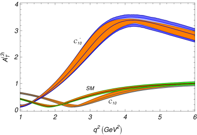
Unfortunately, the simultaneous appearance of , and inside square roots turns the heavy-quark and large-energy limits into rather awkward expressions, not really useful to explain the behaviour of these observables at a glance. Therefore, we only outline their general properties. Equation (56) shows that and play a complementary role, as the numerator of and the denominator of are the same. Thus, when a minimum appears in one of them, a maximum is expected in the other observable and the other way around. This is indeed what can be observed in Fig. 17. For the values of the Wilson coefficients chosen, NP entering can easily be distinguished from the SM curve, displaying a maximum at around 3.5-4 (exactly in the energy region where is showing a minimum), while can only be clearly identified using . Something similar happens with NP entering and : the model-independent values chosen for these Wilson coefficients do not give rise to clear NP signals from , but they can be easily told apart using . In those situations where the origin of the NP curve can not be clearly established using a single observable (for instance, the curve in the plot of Fig. 17 is very similar to the curve), the combined use of , , , and maybe enables us to identify which Wilson coefficient(s) has a contribution from NP.
7 Conclusion
In this paper we have presented how the decay can provide detailed knowledge of NP effects in the flavour sector. We developed a method for constructing observables with specific sensitivity to some types of NP while, at the same time, keeping theoretical errors from form factors under control. A method based on infinitesimal symmetries was presented which allows in a generic way to identify if an arbitrary combination of spin amplitudes is an observable of the angular distribution. For the case of massless leptons we identified the explicit form of all four symmetries present. We showed the possible impact of the unknown corrections on the NP sensitivity of the various angular observables in a systematic way using an ensemble method. Experimental sensitivity to the observables was evaluated for datasets corresponding to 10 of data at LHCb. Using these tools, we did a phenomenological analysis for both -conserving and -violating observables. The conclusion from this is that the -violating observables have very poor experimental sensitivity while the -conserving observables (with ) are very powerful for finding NP, including situations with large weak phases.
Acknowledgments.
JM acknowledges financial support from FPA2005-02211, 2005-SGR-00994, MR from the Universitat Autònoma de Barcelona, UE and WR from the Science and Technology Facilities Council (STFC), and TH from the European network Heptools. TH thanks the CERN theory group for its hospitality during his visits to CERN.Appendix A Kinematics
Assuming the to be on the mass shell, the decay is completely described by four independent kinematic variables; namely, the square of the lepton-pair invariant mass, , and the three angles , and . The sign of the angles for the decay shows great variation in the literature. Therefore we present here an explicit definition of our conventions and point out where the same or different definitions have been used.
First we consider the decay. The angle is the angle between the momentum in the rest frame of the dimuon and the direction of the dimuon in the rest frame of the . The angle is in a similar way the angle between the momentum in the rest frame and the direction of the in the rest frame of the .
Let us for define the momentum vectors
| (57) | |||||
| (58) | |||||
| (59) | |||||
| (60) |
In the dimuon rest frame, we have that the momentum is parallel to and also that points in the opposite direction of the dimuon in the rest frame. Thus we can compute the angle as
| (61) |
where the superscript is used to indicate the frame. In a similar way we have in the rest frame
| (62) |
Finally, if we go to the rest frame of the , we have as the signed angle between the planes defined by the two muons and the decay products respectively. Vectors perpendicular to the decay planes are
| (63) |
which lets us define from
| (64) |
The angles are defined in the intervals
| (65) |
The definition given here is identical to [6] but is different to [7]. However, the two definitions result in the same signs for all the coefficients in Eq. (4).
Now for the decay the angle is still specified with respect to the while for the angle is for the . This is equivalent to what is done in [7]. As the angle does not change the sign of the lepton, we have
| (66) |
in the full-angular distribution in the absence of violation.
For the experimental papers [1, 2], a definition has been adopted where all angular distributions have been plotted for the decay, with the events overlaid assuming conservation. In practise this means that events have the sign of reversed before plotting. When experiments progress to measuring the angle as well, special care needs to be taken to get the definitions correct.
Appendix B Theoretical input parameters and uncertainties
To compute the soft form factor error bands in Figs. 5 and 6 in a conservative fashion, we have used, as input data, the values of and shown in Table 2. One can notice that the value has been taken from [7], as it is compatible to used in [14], while for we have kept the value from [14] to allow for a wider uncertainty range.
The -dependence of the form factors , and has been parametrised according to [28]
| (67) |
where , and are the fit parameters shown in Table 3 of [28]. Substituting the outcomes of Eq. (67) into [14]
| (68) |
we can obtain both the central value and the associated uncertainty curves for and in the - range. These are used to get the fitting parameters , , and of
| (69) |
where within a per mille precision. This parametrisation follows closely Eq. (47) in [13] and allows us to explore the impact of and (with their corresponding uncertainties) to the -violating and -conserving observables studied throughout this paper.
The next step is to compute the amplitudes, keeping one soft form factor fixed at the central value and varying the other in the range allowed by its uncertainty. From them, the observables can be obtained in a straightforward way and the errors added in quadrature.
To generate the theoretical error bands not due to corrections (plotted as the inner orange strips in the plots of Secs. 5 and 6) we have used the criteria of Beneke et al. in [13] and added the following uncertainties in quadrature: the renormalisation scale uncertainty has been found by varying between and (where is the scale at which the Wilson Coefficients, and the masses are evaluated), the uncertainty in the ratio by varying this quantity between 0.29 and 0.31, and the other parametric uncertainties have been collected into the factor [6]
| (70) |
that determines the relative magnitude of the hard-scattering versus the form factor term [13], which is uncertain by about . In our numerical analysis we have used the values of the Wilson coefficients in Table 1 of Ref. [13].
References
- [1] BELLE Collaboration, J. T. Wei et. al., Measurement of the Differential Branching Fraction and Forward-Backward Asymmetry for , Phys. Rev. Lett. 103 (2009) 171801, [arXiv:0904.0770].
- [2] BABAR Collaboration, B. Aubert et. al., Measurements of branching fractions, rate asymmetries, and angular distributions in the rare decays and , Phys. Rev. D73 (2006) 092001, [hep-ex/0604007].
- [3] A. Bharucha and W. Reece, Constraining new physics with in the early LHC era, arXiv:1002.4310.
- [4] F. Kruger and J. Matias, Probing new physics via the transverse amplitudes of at large recoil, Phys. Rev. D71 (2005) 094009, [hep-ph/0502060].
- [5] E. Lunghi and J. Matias, Huge right-handed current effects in in supersymmetry, JHEP 04 (2007) 058, [hep-ph/0612166].
- [6] U. Egede, T. Hurth, J. Matias, M. Ramon, and W. Reece, New observables in the decay mode , JHEP 11 (2008) 032, [arXiv:0807.2589].
- [7] W. Altmannshofer et. al., Symmetries and Asymmetries of Decays in the Standard Model and Beyond, JHEP 01 (2009) 019, [arXiv:0811.1214].
- [8] D. Melikhov, N. Nikitin, and S. Simula, Probing right-handed currents in transitions, Phys. Lett. B442 (1998) 381–389, [hep-ph/9807464].
- [9] C. Bobeth, G. Hiller, and G. Piranishvili, CP Asymmetries in and Untagged , Decays at NLO, JHEP 07 (2008) 106, [arXiv:0805.2525].
- [10] F. Kruger, L. M. Sehgal, N. Sinha, and R. Sinha, Angular distribution and CP asymmetries in the decays and , Phys. Rev. D61 (2000) 114028, [hep-ph/9907386].
- [11] C. S. Kim, Y. G. Kim, C.-D. Lu, and T. Morozumi, Azimuthal angle distribution in at low invariant region, Phys. Rev. D62 (2000) 034013, [hep-ph/0001151].
- [12] A. Faessler, T. Gutsche, M. A. Ivanov, J. G. Korner, and V. E. Lyubovitskij, The Exclusive rare decays K(K*) and D(D*) in a relativistic quark model, Eur. Phys. J. direct C4 (2002) 18, [hep-ph/0205287].
- [13] M. Beneke, T. Feldmann, and D. Seidel, Systematic approach to exclusive , decays, Nucl. Phys. B612 (2001) 25–58, [hep-ph/0106067].
- [14] M. Beneke, T. Feldmann, and D. Seidel, Exclusive radiative and electroweak and penguin decays at NLO, Eur. Phys. J. C41 (2005) 173–188, [hep-ph/0412400].
- [15] J. Charles, A. Le Yaouanc, L. Oliver, O. Pene, and J. C. Raynal, Heavy-to-light form factors in the heavy mass to large energy limit of QCD, Phys. Rev. D60 (1999) 014001, [hep-ph/9812358].
- [16] M. Beneke and T. Feldmann, Symmetry-breaking corrections to heavy-to-light meson form factors at large recoil, Nucl. Phys. B592 (2001) 3–34, [hep-ph/0008255].
- [17] LHCb Collaboration, B. Adeva et. al., Roadmap for selected key measurements of LHCb, arXiv:0912.4179.
- [18] M. Patel and H. Skottowe, A Fisher discriminant selection for at LHCb, Tech. Rep. LHCb-2009-009. CERN-LHCb-2009-009, CERN, Geneva, Jan, 2010.
- [19] F. Krüger, The Discovery potential of a Super Factory. Proceedings, SLAC Workshops, Stanford, USA, 2003, Chapter 2.17, hep-ph/0503261.
- [20] G. Valencia, Constructing CP odd observables, hep-ph/9411441.
- [21] G. Buchalla, G. Hiller, and G. Isidori, Phenomenology of nonstandard couplings in exclusive semileptonic transitions, Phys. Rev. D63 (2000) 014015, [hep-ph/0006136].
- [22] F. Kruger and E. Lunghi, Looking for novel CP violating effects in , Phys. Rev. D63 (2001) 014013, [hep-ph/0008210].
- [23] G. Burdman and G. Hiller, Semileptonic form-factors from decays in the large energy limit, Phys. Rev. D63 (2001) 113008, [hep-ph/0011266].
- [24] B. Stech, Form-factor relations for heavy to light transitions, Phys. Lett. B354 (1995) 447–452, [hep-ph/9502378].
- [25] J. M. Soares, Form factor relations for heavy-to-heavy and heavy-to- light meson transitions, Phys. Rev. D54 (1996) 6837–6841, [hep-ph/9607284].
- [26] J. M. Soares, Form factor relations for heavy-to-light meson transitions: Tests of the quark model predictions, hep-ph/9810421.
- [27] A. K. Alok et. al., New-physics contributions to the forward-backward asymmetry in , JHEP 02 (2010) 053, [arXiv:0912.1382].
- [28] P. Ball and V. M. Braun, Exclusive semileptonic and rare meson decays in QCD, Phys. Rev. D58 (1998) 094016, [hep-ph/9805422].
- [29] Particle Data Group Collaboration, C. Amsler et. al., Review of particle physics, Phys. Lett. B667 (2008) 1.
- [30] O. Buchmuller and H. Flacher, Fits to moment measurements from and decays using heavy quark expansions in the kinetic scheme, Phys. Rev. D73 (2006) 073008, [hep-ph/0507253].
- [31] K. Zyablyuk, Gluon condensate and -quark mass in pseudoscalar sum rules at 3-loop order, JHEP 01 (2003) 081, [hep-ph/0210103].
- [32] T. Onogi, Heavy flavor physics from lattice QCD, PoS LAT2006 (2006) 017, [hep-lat/0610115].
- [33] P. Ball, V. M. Braun, and A. Lenz, Twist-4 Distribution Amplitudes of the and Mesons in QCD, JHEP 08 (2007) 090, [arXiv:0707.1201].
- [34] P. Ball and R. Zwicky, from , JHEP 04 (2006) 046, [hep-ph/0603232].