Magnetic order in a spin-1/2 interpolating kagome-square Heisenberg antiferromagnet

Abstract

The coupled cluster method is applied to a spin-half model at zero temperature ($T=0$), which interpolates between Heisenberg antiferromagnets (HAF’s) on a kagome and a square lattice. With respect to an underlying triangular lattice the strengths of the Heisenberg bonds joining the nearest-neighbor (NN) kagome sites are $J_{1}\geq 0$ along two of the equivalent directions and $J_{2}\geq 0$ along the third. Sites connected by $J_{2}$ bonds are themselves connected to the missing NN non-kagome sites of the triangular lattice by bonds of strength $J_{1}^{\prime}\geq 0$. When $J_{1}^{\prime}=J_{1}$ and $J_{2}=0$ the model reduces to the square-lattice HAF. The magnetic ordering of the system is investigated and its $T=0$ phase diagram discussed. Results for the kagome HAF limit are among the best available.

I Introduction

Quantum magnets defined on two-dimensional (2D) spin lattices exhibit a wide range of physical states at zero temperature, from those with classical-type ordering (albeit reduced by quantum fluctuations) to valence-bond solids and spin liquids.2D_magnetism_1 ; 2D_magnetism_2 The behavior of these strongly correlated and often highly frustrated systems is driven by the nature of the underlying crystallographic lattice, by the number and range of the magnetic bonds, and by the spin quantum numbers of the atoms localized to the lattice sites. Very few exact results exist for such 2D systems and the application of approximate methods has become crucial to their understanding. A complete picture of their behavior has only slowly begun to emerge by considering a wide range of possible scenarios in related models that are themselves often inspired, or followed closely afterwards, by their experimental realisation and study. For easy and accurate comparisons to be made it is clearly preferable to use the same theoretical technique. Among the most accurate, most universally applicable, and most widely applied to quantum magnets of such methods is the coupled cluster method (CCM).Bi:1991 ; Ze:1998 ; Fa:2004 Our aim here is to use the CCM to extend our understanding of frustrated quantum magnets by applying it to a novel 2D system that, in some well-defined sense described below, interpolates between Heisenberg antiferromagnets (HAF’s) defined on square and kagome lattices respectively.

An archetypal and much studied model in quantum magnetism is the frustrated spin-half $J_{1}$–$J_{2}$ HAF model on the square lattice with nearest-neighbor (NN) bonds (of strength $J_{1}>0$) competing with next-nearest-neighbor (NNN) bonds (of strength $J_{2}\equiv\alpha J_{1}>0$). It exhibits two different quasiclassical phases with collinear magnetic long-range order (LRO) at small ($\alpha<\alpha_{c_{1}}\approx 0.4$) and large ($\alpha>\alpha_{c_{2}}\approx 0.6$) values of $\alpha$, separated by an intermediate quantum paramagnetic phase with no magnetic LRO in the regime $\alpha_{c_{1}}<\alpha<\alpha_{c_{2}}$. Interest in this model has been reinvigorated of late by its experimental realisation in such layered magnetic materials as Li₂VOSiO₄,Mel:2000 ; Ro:2002 Li₂VOGeO₄,Mel:2000 VOMoO₄,Bom:2005 and BaCdVO(PO₄)₂.Na:2008 The syntheses of such layered quasi-2D materials has stimulated a great deal of renewed interest in the model (and see, e.g., (Refs. [Ca:2000, ; Ca:2001, ; Sin:2003, ; Ro:2004, ]). Amongst several methods applied to the $J_{1}$–$J_{2}$ model has been the CCM.j1j2_square_ccm1 ; Bi:2008_PRB ; Bi:2008_JPCM ; j1j2_square_ccm5 ; j1j2_square_ccm4

In view of the huge interest in the $J_{1}$–$J_{2}$ model there have been several recent attempts to investigate various generalizations and modifications of the model, in order to shed further light on its properties. As an example of a generalization of the model we mention a recent study Schm:2006 of the effects of interlayer couplings on the 2D $J_{1}$–$J_{2}$ model. This study also employed the CCM in its analysis. Modifications of the $J_{1}$–$J_{2}$ model that have been studied include models wherein some of the NNN $J_{2}$ bonds are removed. Various such models exist in which either half or three-quarters of the $J_{2}$ bonds are removed in particular arrangements, as discussed below. All of these models studied to date have fascinating magnetic properties and ground-state phases in their own right.

One such model is the spin-half anisotropic HAF on the 2D triangular lattice, which has also been studied by the CCM,square_triangle and which interpolates between HAF’s on square and triangular lattices. It is fully equivalent to a variant of the square-lattice $J_{1}$–$J_{2}$ model in which half of the $J_{2}$ bonds are removed, leaving just one NNN bond across the same diagonal of each basic square plaquette. Thus, for this model, the two cases $J_{2}=0$ and $J_{2}\rightarrow\infty$ relate to a HAF on the square lattice and a set of decoupled one-dimensional HAF chains respectively, with the HAF on the triangular lattice in between at $J_{2}=J_{1}$. Strong evidence was foundsquare_triangle that quantum fluctuations for this spin-half model favor a weakly first-order (or possibly second-order) transition from Néel order to a helical state at a first critical point at $\alpha_{c_{1}}=0.80\pm 0.01$ by contrast with the corresponding second-order transition between the equivalent classical states at $\alpha_{{\rm cl}}=0.5$. The CCM was also, uniquely, powerful enough to provide strong evidence for a second quantum critical point at $\alpha_{c_{2}}=1.8\pm 0.4$ where a first-order transition occurs between the helical phase and a collinear stripe-ordered phase with no classical counterpart, thereby providing quantitative verification of an earlier qualitative prediction of such a transition from a renormalization group analysis of the model.St:2007 (As a parenthetical note, a different way of removing half the $J_{2}$ bonds, results in the so-called Union Jack model, to which the CCM has also recently been applied,UJack_ccm and which has a quite different zero-temperatue phase diagram).

A further modification of the original spin-half $J_{1}$–$J_{2}$ model is now to remove another half of the $J_{2}$ bonds, leaving half the fundamental square plaquettes with one $J_{2}$ bond and the other half with none. One way of doing this in a regular fashion results in the Shastry-Sutherland modelshastry1 in which no $J_{2}$ bonds meet at any lattice site and every site is five-connected (by four NN $J_{1}$ bonds and one $J_{2}$ bond). Interest in this model has been renewed by the discovery of the magnetic material $\mathrm{SrCu}_{2}(\mathrm{BO}_{3})_{2}$ [Ref. Ka:1999, ] that can be understood in terms of it. Its classical ground state is the collinear Néel state for $J_{2}/J_{1}\leq 1$ and a noncollinear spiral for $J_{2}/J_{1}>1$, with a second-order phase transition in between. However, it is known that the spin-half model has a quantum ground state which is a product of local pair singlets (the so-called orthogonal-dimer state) for $J_{2}/J_{1}\geq 1.465\pm 0.025$, which has no classical counterpart. The CCM has also been applied to this modelshastry2 ; shastry3 and the latest resultsshastry3 strongly suggest that no intermediate phase exists between the Néel and dimerized phases, and that the direct transition between them is of first-order type.

A different, but equally important, archetypal magnetic system showing frustration, but now of the geometric kind rather than the dynamic kind, is the spin-half kagome-lattice HAF. Although this system has been the subject of intense study over a long period, the nature of its gound state is still not definitively settled. Among the leading theoretical contenders are a valence-bond solid stateMar:1991 ; Syr:2002 ; Nik:2003 ; Bud:2004 ; Sin:2007 ; Eve:2010 and a spin-liquid state.Sach:1992 ; Leung:1993 ; Lech:1997 ; Mila:1998 ; Wald:1998 ; Hast:2000 ; Mamb:2000 ; Herm:2005 ; Wang:2006 ; Ran:2007 ; Herm:2008 ; Jiang:2008 The spin-half kagome-lattice HAF has become the subject of renewed interest after a possible physical realization of the model has been found experimentally in the herbertsmithite material ZnCu₃(OH)₆Cl₂.Helton:2007 ; Vdries:2008 A spatially anisotropic version of the spin-half kagome-lattice HAF has also been experimentally studied after its physical realization in the volborthite material Cu₃V₂O₇(OH)₂$\cdot$2H₂O.Yoshida:2009 This latter model has also been studied theoretically in recent years.Yavo:2007 ; Wang:2007 ; Kagome_Schn:2008

In the present paper we investigate the phase diagram of a novel spin-half HAF that is another depleted modification of the $J_{1}$–$J_{2}$ model, and which also contains both the spatially anisotropic and the isotropic kagome-lattice HAF’s discussed above as limiting cases. As described in more detail below the model also interpolates continuously between the geometrically frustrated kagome-lattice HAF and the unfrustrated square-lattice HAF. After describing the model in Sec. II, we apply the CCM to investigate its ground-state properties. The CCM is first described briefly in Sec. III, and the results are presented in Sec. IV. We conclude in Sec. V with a discussion of the results and a comparison of them with other results for limiting cases of our model.

II The model

In this paper we consider an alternate and novel variant of the $J_{1}$–$J_{2}$ model in which three-quarters of the $J_{2}$ bonds are removed from the original $J_{1}$–$J_{2}$ model as in the Shastry-Sutherland model above, but in a different pattern, as shown in Fig. 1.

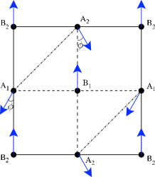
(a) Canted

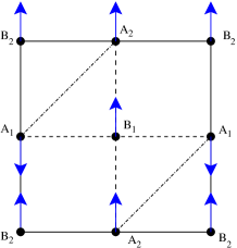
(b) Semi-striped

Figure 1: (Color online) The interpolating kagome-square model; — $J_{1}$; - - $J_{1}^{\prime}$; - $\cdot$ - $J_{2}$; showing (a) the canted state; and (b) the semi-striped state.

It may equivalently be obtained from the spin-half anisotropic HAF on the 2D triangular lattice by removing every second line of NNN $J_{2}$ bonds. The square-lattice representation of the model shown in Fig. 1 contains the two square sublattices of A sites and B sites respectively, and each of these in turn contains the two square sublattices of ${\rm A}_{1}$ and ${\rm A}_{2}$ sites, and ${\rm B}_{1}$ and ${\rm B}_{2}$ sites respectively, as shown. It is very illuminating to consider the anisotropic variant in which half of the $J_{1}$ bonds are allowed to have the strengths $J_{1}^{\prime}>0$ along alternating rows and columns. All of the bonds joining sites $i$ and $j$ are of standard Heisenberg type, i.e., proportional to s_i$\cdot$s_j, where the operators s${}_{i}=(s_{i}^{x},s_{i}^{y},s_{i}^{z})$ are the quantum spin operators on lattice site $i$, with s${}_{i}^{2}=s(s+1)$ and $s=\frac{1}{2}$ for the quantum case considered here.

This so-called interpolating kagome-square model differs principally from the Shastry-Sunderland model in that the A sites are six-connected (by 2 NN $J_{1}$ bonds, 2 NN $J_{1}^{\prime}$ bonds and 2 NNN $J_{2}$ bonds) while the B sites are four-connected (by four NN $J_{1}^{\prime}$ bonds for the B₁ sites and four NN $J_{1}$ bonds for the B₂ sites). The spin-half HAF’s on the 2D kagome and square lattices are represented respectively by the limiting cases {$J_{1}=J_{2},J_{1}^{\prime}=0$} and {$J_{1}=J_{1}^{\prime},J_{2}=0$}. The limiting case when {$J_{1}=J_{1}^{\prime}=0;J_{2}>0$} represents a set of uncoupled 1D HAF chains. The case $J_{1}^{\prime}=0$ with $J_{2}\neq J_{1}$ represents a spatially anisotropic kagome HAF considered recently by other authors,Yavo:2007 ; Wang:2007 ; Kagome_Schn:2008 especially in the quasi-1D limit where $J_{2}/J_{1}\gg 1$.Kagome_Schn:2008 Henceforth we set $J_{1}\equiv 1$ and consider the case when all bonds are antiferromagnetic, (i.e., $J_{1}^{\prime}\geq 0,J_{2}\geq 0$).

Considered as a classical model (corresponding to the case where the spin quantum number $s\rightarrow\infty$) the interpolating kagome-square model has only two ground-state (gs) phases separated by a continuous (second-order) phase transition at $J_{2}=J_{2}^{{\rm cl}}\equiv\frac{1}{2}(J_{1}+J_{1}^{\prime})$. For $J_{2}<J_{2}^{{\rm cl}}$ the system is Néel-ordered on the square lattice, while for $J_{2}>J_{2}^{{\rm cl}}$ the system has noncollinear canted order as shown in Fig. 1(a), in which the spins on each of the A₁ and the A₂ sites are canted respectively at angles ($\pi\mp\phi$) with respect to those on the B sublattice, all of the latter of which point in the same direction. The lowest-energy state in the canted phase is obtained with $\phi=\phi_{{\rm cl}}\equiv{\rm cos}^{-1}(J_{2}^{{\rm cl}}/J_{2}$). The Néel state, for $J_{2}<J_{2}^{{\rm cl}}$, simply corresponds to the case $\phi_{{\rm cl}}=0$. When $J_{1}^{\prime}=0$ and $J_{2}=J_{1}$, corresponding to the isotropic kagome-lattice HAF, $\phi_{{\rm cl}}=\frac{1}{3}\pi$, as required by symmetry. We also note that as $J_{2}\rightarrow\infty$ (with $J_{1}$ and $J_{1}^{\prime}$ finite), $\phi_{{\rm cl}}\rightarrow\frac{1}{2}\pi$, and the spins on the A sublattice become antiferromagnetically ordered, as is expected, and these spins are orientated at 90^∘ to those on the ferromagnetically-ordered B sublattice. Of course there is complete degeneracy at this classical level in this limit between all states for which the relative ordering directions for spins on the A and B sublattices are arbitrary. The spin-half problem in the same limit should also comprise decoupled ferromagnetic and antiferromagnetic sublattices. We expect that this degeneracy in relative orientation might be lifted by quantum fluctuations by the well-known phenomenon of order-by-disorder.Vi:1977 Since it is also true that quantum fluctuations generally favor collinear ordering, a preferred state is thus likely to be the so-called ferrimagnetic semi-striped state shown in Fig. 1(b) where the A sublattice is now Néel-ordered in the same direction as the B sublattice is ferromagnetically ordered. Alternate rows (and columns) are thus ferromagnetically and antiferromagnetically ordered in the same direction in the semi-striped state.

III Coupled Cluster Method

The CCM (see, e.g., Refs. [Bi:1991, ; Ze:1998, ; Fa:2004, ] and references cited therein) that we employ here is one of the most powerful and most versatile modern techniques available to us in quantum many-body theory. It has been applied very successfully to various quantum magnets (see Refs. [j1j2_square_ccm1, ; Bi:2008_PRB, ; Bi:2008_JPCM, ; j1j2_square_ccm4, ; j1j2_square_ccm5, ; Fa:2001, ; Kr:2000, ; Schm:2006, ; Fa:2004, ; Ze:1998, ; shastry2, ; shastry3, ; square_triangle, ] and references cited therein). The method is particularly appropriate for studying frustrated systems, for which some of the main alternative methods either cannot be applied or are sometimes only of limited usefulness, as explained below. For example, quantum Monte Carlo (QMC) techniques are particularly plagued by the sign problem for such systems, and the exact diagnoalization (ED) method is restricted in practice by available computational power, particularly for $s>1/2$, to such small lattices that it is often insensitive to the details of any subtle phase order present.

The method of applying the CCM to quantum magnets has been described in detail elsewhere (see, e.g., Refs. [Ze:1998, ; Kr:2000, ; Fa:2001, ; Schm:2006, ; j1j2_square_ccm1, ; Fa:2004, ] and references cited therein). It relies on building multispin correlations on top of a chosen gs model state $|\Phi\rangle$ in a systematic hierarchy of LSUB$n$ approximations (described below) for the correlation operators $S$ and $\tilde{S}$ that parametrize the exact gs ket and bra wave functions of the system respectively as $|\Psi\rangle=e^{S}|\Phi\rangle$ and $\langle\tilde{\Psi}|=\langle\Phi|\tilde{S}e^{-S}$. In the work presented here we use two different choices for the model state $|\Phi\rangle$, namely the classical antiferromagnetic Néel state and the ferrimagnetic canted state. We note that the ferrimagnetic semi-striped state provides another possible choice of model state $|\Phi\rangle$, but we do not consider it further in the present paper, except in brief remarks at the end of Sec. IV.

In each case we employ the well-established LSUB$n$ approximation scheme in which all possible multi-spin-flip correlations over different locales on the (square) lattice defined by $n$ or few contiguous lattice sites are retained. As usual the number of independent fundamental clusters (i.e., those that are inequivalent under the symmetries of the Hamiltonian and of the model state) increases rapidly with the truncation index $n$. For example, the number of such fundamental clusters for the canted model state is 201481 at the LSUB8 level of approximation in the triangular-lattice geomery where $J_{2}$ bonds are considered to join NN pairs, and this is the highest level for the present model that we have been able to attain with available computing power. In order to solve the corresponding coupled sets of CCM bra- and ket-state equations we use massively parallel computing,ccm typically using 600 processors simultaneously. We present results below both at various LSUB$n$ levels of approximation with $n=\{2,4,6,8\}$ for the case $J_{1}^{\prime}=J_{1}=1$ and with $n=\{2,4,6\}$ for other values of the bond strengths, and at the corresponding $n\rightarrow\infty$ extrapolation (LSUB$\infty$) based on the well-tested extrapolation schemes described below and in more detail elsewhere.Ze:1998 ; Fa:2004 ; j1j2_square_ccm1 ; Bi:2008_PRB ; Bi:2008_JPCM We note that, as always, the CCM exactly obeys the Goldstone linked-cluster theorem at every LSUB$n$ level of approximation. Hence we work from the outset in the limit $N\rightarrow\infty$, where $N$ is the number of sites on the square lattice, and extensive quantities like the gs energy are hence always guaranteed to be linearly proportional to $N$ in this limit. We note for later purposes that the number of sites on the kagome lattice (obtained by removing all B₁ sites in Fig. 1) is clearly $N_{K}=\frac{3}{4}N$.

Note that for the canted phase we perform calculations for arbitrary canting angle $\phi$ shown in Fig. 1(a), and then minimize the corresponding LSUB$n$ approximation for the energy $E_{{\rm LSUB}n}(\phi)$ with respect to $\phi$ to yield the corresponding approximation to the quantum canting angle $\phi_{{\rm LSUB}n}$. Generally (for $n>2$) the minimization must be carried out computationally in an iterative procedure, and for the highest values of $n$ that we use here the use of supercomputing resources was essential. Results for the canting angle $\phi_{{\rm LSUB}n}$ will be given later.

As always, we choose local spin coordinates on each site for each choice of model state, so that all spins in $|\Phi\rangle$, whatever the choice, point in the negative $z$-direction (i.e., downwards) by definition in these local coordinates. Then, in the LSUB$n$ approximation all possible multi-spin-flip correlations over different locales on the lattice defined by $n$ or fewer contiguous lattice sites are retained. The operator $S$ thus contains only linear sums of products of creation operator $s^{+}_{k}\equiv s^{x}_{k}+is^{y}_{k}$ on various sites $k$, while the operator $\tilde{S}$ contains only similar linear sums of products of destruction operators $s^{-}_{k}\equiv s^{x}_{k}-is^{y}_{k}$. The numbers $N_{f}$ of such distinct (i.e., under the symmetries of the lattice and the model state) fundamental configurations of the current model in various LSUB$n$ approximations are shown in Table 1.

Table 1: Number of fundamental LSUB$n$ configurations ($N_{f}$) for the semi-striped and canted states of the spin-$1/2$ $J_{1}$–$J_{1}^{\prime}$–$J_{2}$ interpolating square-kagome model.

Method	$N_{f}$
	semi-striped	canted
LSUB$2$	3	5
LSUB$4$	32	200
LSUB$6$	645	6041
LSUB$8$	14936	201481

We note that the distinct configurations given in Table 1 are defined with respect to the geometry described in Sec. II, and in which the B sublattice sites of Fig. 1(a) are defined to have four NN sites joined to them by either $J_{1}$ bonds or $J_{1}^{\prime}$ bonds, and the A sublattice sites are defined to have the six NN sites joined to them by $J_{1}$, $J_{1}^{\prime}$, or $J_{2}$ bonds. If we had chosen instead to work in the square-lattice geometry every site would have four NN sites.

A significant extra computational burden arises here for the canted state due to the need to optimize the quantum canting angle $\phi$ at each LSUB$n$ level of approximation, as described above. Furthermore, for many model states the quantum number $s^{z}_{T}\equiv\sum^{N}_{i=1}s^{z}_{i}$ in the original global spin-coordinate frame, may be used to restrict the numbers of fundamental multi-spin-flip configurations to those clusters that preserve $s^{z}_{T}$ as a good quantum number. This is true for the Néel state where $s^{z}_{T}=0$ and for the semi-striped state for which $s^{z}_{T}=\frac{1}{2}Ns$, where $N$ is the number of lattice sites. However, for the canted model state that symmetry is absent, which largely explains the significantly greater number of fundamental configurations shown in Table 1 for the canted state at a given LSUB$n$ order. Hence, the maximum LSUB$n$ level that we can reach here for the canted state, even with massive parallelization and the use of supercomputing resources, is LSUB$8$. For example, to obtain a single data point for a given value of $J_{2}$, with $J_{1}=1$ and $J_{1}^{\prime}=1$, for the canted phase at the LSUB$8$ level typically required about 0.2-2.0 h computing time using 600 processors simultaneously for non-critical regions. However, for values of $J_{2}$ near to critical points, the LSUB8 computing time increased significantly, typically to lie in the range of 5-24 h to obtain a single data point using 600 processors simultaneously.

At each level of approximation we may then calculate a corresponding estimate of the gs expectation value of any physical observable such as the energy $E$ and the magnetic order parameter, $M\equiv-\frac{1}{N}\sum^{N}_{i=1}\langle\tilde{\Psi}|s^{z}_{i}|\Psi\rangle$, defined in the local, rotated spin axes, and which thus represents the average on-site magnetization. Note that $M$ is just the usual sublattice (or staggered) magnetization per site for the case of the Néel state as the CCM model state, for example.

It is important to note that we never need to perform any finite-size scaling, since all CCM approximations are automatically performed from the outset in the infinite-lattice limit, $N\rightarrow\infty$, where $N$ is the number of lattice sites. However, we do need as a last step to extrapolate to the exact $n\rightarrow\infty$ limit in the LSUB$n$ truncation index $n$, at which the complete (infinite) Hilbert space is reached. We use here the well-tested Fa:2001 ; Kr:2000 empirical scaling laws

$$E/N=a_{0}+a_{1}n^{-2}+a_{2}n^{-4}\,,$$ (1)

$$M=b_{0}+b_{1}n^{-1}+b_{2}n^{-2}\,.$$ (2)

IV Results

We show in Fig. 2

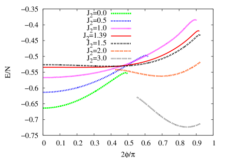
Figure 2: (Color online) Ground-state energy per spin of the spin-1/2 interpolating kagome-square model with $J_{1}=J_{1}^{\prime}=1$, using the LSUB4 approximation of the CCM with the canted model state, versus the canting angle $\phi$. For $J_{2}\lesssim 1.392$ the minimum is at $\phi=0$ (Néel order) at this level of approximation, whereas for $J_{2}\gtrsim 1.392$ the minimum occurs at $\phi=\phi_{{\rm LSUB}4}\neq 0$, indicating a phase transition at $J_{2}\approx 1.392$ in this approximation. Results are shown for those values of $\phi$ for which the corresponding CCM equations have real solutions.

our CCM results, based on the canted model state, for the gs energy per spin, $E/N$, plotted as a function of the canting angle $\phi$. We show results specifically at the LSUB4 level of approximation for the case $J_{1}=J_{1}^{\prime}=1$, but our results are qualitatively similar at other LSUB$n$ levels and for other values of $J_{1}^{\prime}$ (with $J_{1}=1$). Curves like those in Fig. 2 show that at this LSUB4 level of approximation, with $J_{1}=J_{1}^{\prime}=1$, the minimum energy is at $\phi=0$ for $J_{2}<J_{2}^{{\rm LSUB}4}\approx 1.392$ and at a value $\phi\neq 0$ for $J_{2}>J_{2}^{{\rm LSUB}4}$. Thus, we have a clear indication of a shift of the critical point at $J_{2}=J_{2}^{c_{1}}$ between the quantum Néel and canted phases from the classical value $J_{2}^{{\rm cl}}=1$ when $J_{1}=J_{1}^{\prime}=1$. The observation that Néel order survives beyond the classically stable regime, for the quantum spin-half system, is an example of the promotion of collinear order by quantum fluctuations, a phenomenon that has been observed in many other systems.

In Fig. 3

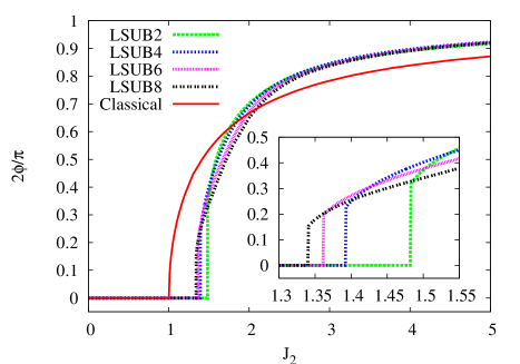
Figure 3: (Color online) The angle $\phi_{{\rm LSUB}n}$ that minimizes the energy $E_{{\rm LSUB}n}(\phi)$ of the spin-half interpolating kagome-square model with $J_{1}=J_{1}^{\prime}=1$, versus $J_{2}$. The LSUB$n$ approximations with $n=\{2,4,6,8\}$, using the canted model state, are shown. The corresponding classical result $\phi_{{\rm cl}}$ is shown for comparison.

we show the canting angle $\phi_{{\rm LSUB}n}$ that minimizes the gs energy $E_{{\rm LSUB}n}$($\phi$) at various CCM LSUB$n$ levels based on the canted state as model state, with $n=\{2,4,6,8\}$, again for the case $J_{1}^{\prime}=J_{1}=1$. We see clearly that at each LSUB$n$ level shown there is a finite jump in $\phi_{{\rm LSUB}n}$ at the corresponding LSUB$n$ approximation for the phase transition at $J_{2}=J_{2}^{{\rm LSUB}n}$ between the Néel state (with $\phi_{{\rm LSUB}n}=0$) and the canted state (with $\phi_{{\rm LSUB}n}\neq 0$). Thus at each LSUB$n$ level of approximation the quantum phase transition is first-order, compared to the second-order classical counterpart. A close inspection of the insert in Fig. 3 shows that we cannot completely rule out as $n\rightarrow\infty$, with increasing level of LSUB$n$ approximation, the possibility that the phase transition at $J_{2}=J_{2}^{c_{1}}\equiv J_{2}^{{\rm LSUB}\infty}$ becomes of second-order type, although a weakly first-order one seems more likely on the evidence so far. We note that the LSUB$n$ estimates for the phase transition between Néel and canted phases, $J_{2}^{{\rm LSUB}n}$, fit well to an extrapolation scheme $J_{2}^{{\rm LSUB}n}=J_{2}^{{\rm LSUB}\infty}+cn^{-1}$. The corresponding estimates for $J_{2}^{c_{1}}=J_{2}^{{\rm LSUB}\infty}$ in the case shown ($J_{1}=J_{1}^{\prime}=1$) are $J_{2}^{c_{1}}=1.298\pm 0.003$ based on $n=\{2,4,6,8\}$ and $J_{2}^{c_{1}}=1.302\pm 0.001$ based on $n=\{2,4,6\}$ where the errors quoted are those associated with the specific fit determined via least-squares. We also see from Fig. 3 that results for the quantum canting angle converge very rapidly with increasing LSUB$n$ level of approximation, except for a small region near the phase transition at $J_{2}=J_{2}^{c_{1}}$. We note too that as $J_{2}\rightarrow\infty$ the canting angle $\phi\rightarrow\frac{1}{2}\pi$ considerably faster than does the classical analog $\phi_{{\rm cl}}$. Similar estimates for $J_{2}^{c_{1}}$ have been calculated for other values of $J_{1}^{\prime}$ (with $J_{1}\equiv 1$). Thus in Fig. 4

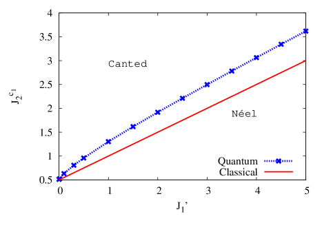
Figure 4: Ground-state phase diagram of the spin-half interpolating square-kagome lattice model, calculated as described in the text, compared with its classical counterpart.

we compare the phase boundary between the Néel and canted states for the present spin-half model with its classical analog. We note in particular that at $J_{1}^{\prime}=0$ the critical value calculated as above is at $J_{2}^{c_{1}}=0.51\pm 0.01$, compared with the classical value $J_{2}^{{\rm cl}}=0.5$ at $J_{1}^{\prime}=0$.

Our CCM results for the gs energy per spin, $E/N$, are shown in Fig. 5

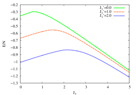
Figure 5: (Color online) Ground-state energy per spin versus $J_{2}$ for the Néel and canted phases of the spin-1/2 interpolating kagome-square model ($J_{1}=1$). The CCM LSUB$\infty$ results based on LSUB$n$ approximations with $n=\{2,4,6,8\}$ for $J_{1}^{\prime}=1.0$ and with $n=\{2,4,6\}$ for the other two $J_{1}^{\prime}$ values, are shown. The CCM results using the canted model state are based on extrapolated LSUB$n$ approximations with the canting angle $\phi=\phi_{{\rm LSUB}n}$ that minimizes $E_{{\rm LSUB}n}(\phi)$.

as a function of $J_{2}$, for various values of $J_{1}^{\prime}$ (with $J_{1}=1$). (Note that for the case $J_{1}^{\prime}=0$, we typically use a very small value $J_{1}^{\prime}\approx 10^{-5}$.) At the isotropic kagome point ($J_{1}^{\prime}=0,J_{2}=J_{1}=1$) the gs energy per spin is $E/N\approx-0.324\pm 0.002$, where the error estimate is based on comparing LSUB$n$ extrapolations from the three sets $n=\{2,4,6,8\}$, $\{2,4,6\}$, and $\{4,6,8\}$. Expressed equivalently in terms of the number $N_{K}$ of kagome sites, this result is $E/N_{K}\approx-0.432\pm 0.002$. Our corresponding result for the pure square-lattice HAF (with $J_{1}^{\prime}=J_{1}=1,J_{2}=0$) is $E/N\approx-0.6697\pm 0.0003$. One observes weak signals of a discontinuity in the first derivative of the energy at the phase transition points $J_{2}^{c_{1}}$ for all values of $J_{1}^{\prime}$.

Much clearer evidence of a first-order phase transition at $J_{2}^{c_{1}}$ is seen in Fig. 6

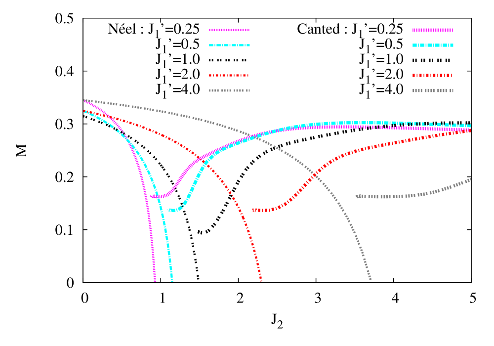
(a) $J_{1}^{\prime}=0.25,0.5,1.0,2.0,4.0$

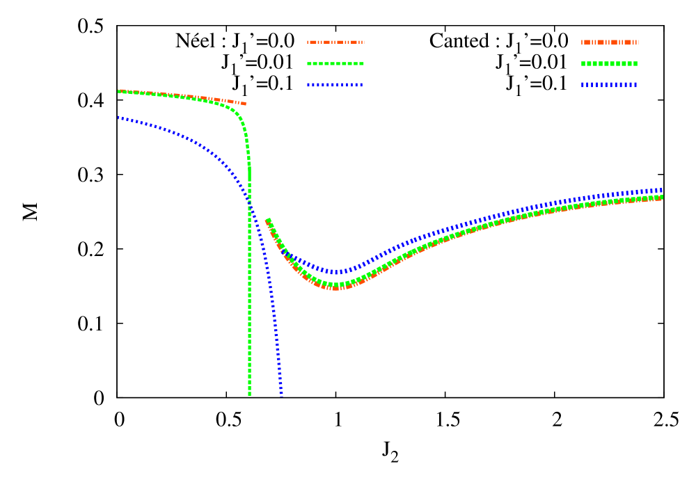
(b) $J_{1}^{\prime}=0.0,0.01,0.1$

Figure 6: (Color online) Ground-state magnetic order parameter versus $J_{2}$ for the Néel and canted phases of the spin-half interpolating kagome-square model ($J_{1}=1$). The CCM LSUB$\infty$ results based on LSUB$n$ approximations with $n=\{2,4,6,8\}$ for $J_{1}^{\prime}=1.0$ and with $n=\{2,4,6\}$ for the other $J_{1}^{\prime}$ values, are shown. The CCM results using the canted model state are based on extrapolated LSUB$n$ approximations with the canting angle $\phi=\phi_{{\rm LSUB}n}$ that miniminizes $E_{{\rm LSUB}n}(\phi)$.

where we show comparable CCM results for the average on-site magnetization or magnetic order parameter, $M$ defined in Sec. III. From the symmetry of the model under the interchange of the bonds $J_{1}\rightleftharpoons J_{1}^{\prime}$, we note that the order parameter should satisfy the relation $M(J_{1},J_{1}^{\prime},J_{2})=M(J_{1}^{\prime},J_{1},J_{2}$). Since the order parameter is independent of an overall scaling of the Hamiltonian, we may also express this relation in the form $M(1,J_{1}^{\prime}/J_{1},J_{2}/J_{1})=M(1,J_{1}/J_{1}^{\prime},J_{2}/J_{1}^{\prime})$. Thus, placing $J_{1}\equiv 1$, as we have done here, and considering $M=M(J_{1}^{\prime};J_{2})$ as a function of the remaining two parameters, we have the exact relation $M(J_{1}^{\prime};J_{2})=M(1/J_{1}^{\prime};J_{2}/J_{1}^{\prime}$). The curves shown in Fig. 6(a) for $J_{1}^{\prime}=0.25$ and 4.0 and for 0.5 and 2.0 are easily seen to satisfy this relation for both the Néel and canted phases, thereby providing a very good check on our numerics.

For the anisotropic kagome lattice ($J_{1}^{\prime}=0$), the minimum LSUB$\infty$ value of $M\approx 0.145$ is seen from Fig. 6(b) to occur precisely at the isotropic kagome HAF point ($J_{1}^{\prime}=0,J_{2}=J_{1}=1$). We may easily re-express this at the kagome point $J_{1}^{\prime}=0$ in terms of $M_{K}\equiv-\frac{1}{N_{K}}\sum^{N_{K}}_{i=1}\langle s^{z}_{i}\rangle$, where the sum is taken only over the kagome-lattice sites and where again the spins are defined in the local, rotated spin axes in which all spins in the CCM model state point in the negative z-direction. Thus, the non-kagome spins on the B₁ sites are then frozen in the case $J_{1}^{\prime}=0$ to have their spins exactly aligned along the local z-axes, and hence at the kagome point $M_{K}=\frac{4}{3}(M-0.125)\approx 0.026$. Our result is thus that only 5% of the classical ordering remains for the spin-half kagome HAF, with an error that makes this compatible with zero. Our corresponding result for the square-lattice HAF is $M=0.310\pm 0.003$.

For the Néel phase ($\phi=0$) curves in Fig. 6 we show the extrapolated (LSUB$\infty$) results for all values of $J_{2}$ (and given values of $J_{1}$ and $J_{1}^{\prime}$) for which $M>0$, and hence these extend into a regime that is unphysical for the Néel phase since the canted phase has lower energy there. By contrast, for the canted phase ($\phi\neq 0$) curves in Fig. 6 we show only the extrapolated (LSUB$\infty$) results for regimes of $J_{2}$ (and given values of $J_{1}$ and $J_{1}^{\prime}$) for which we have LSUB$n$ data (with $\phi_{{\rm LSUB}n}\neq 0$) for all of the set $n=\{2,4,6\}$, in order that the $n\rightarrow\infty$ extrapolation can be robustly performed. Curves like those in Fig. 3 thus show that the results for the canted phase shown in Fig. 6 terminate (artificially) at $J_{2}^{{\rm LSUB}2}>J_{2}^{{\rm LSUB}_{\infty}}=J_{2}^{c_{1}}$, rather than at the physical value $J_{2}^{c_{1}}$. For this (unphysical, but computationally imposed) reason, corresponding pairs of curves for $M$ versus $J_{2}$ (for the same given values of $J_{1}$ and $J_{1}^{\prime}$) for the Néel and canted phases do not meet. We note, however, that simple (spline) extrapolations of the LSUB$\infty$ canted-phase magnetization curves generally give corresponding estimates for $J_{2}^{c_{1}}$ at which they meet their Néel-phase counterparts, which are in excellent agreement with those calculated as in Fig. 3. Such extrapolations also give clear evidence that the order parameter curves for the two phases meet at a value $J_{2}=J_{2}^{c_{1}}$ at which $M$ is nonzero (and hence the transition is of first-order type) for all values of $J_{1}^{\prime}$, and furthermore that the curves have no discontinuity in slope (or only a very small one) at $J_{2}=J_{2}^{c_{1}}$.

We remark that the one region where the extrapolation procedure for $M$ becomes slightly problematic is for values of $J_{1}^{\prime}\lesssim 0.1$ near the (generally anisotropic) kagome point, $J_{1}^{\prime}=0$. The reason is clear from Fig. 6(b) since the Néel curves drop to zero from a nonzero value with a slope that approaches infinity as $J_{1}^{\prime}\rightarrow 0$. Thus, the Néel curves for the $J_{1}^{\prime}=0$ case extend (artificially) to the end-point $J_{2}^{{\rm LSUB}6}\approx 0.592$, whereas we know the value $J_{2}^{{\rm LSUB}\infty}\approx 0.51$ in this case. Clearly, the nature of the transition becomes rather singular in the limit $J_{1}^{\prime}\rightarrow 0$, as Fig. 6(b) clearly shows.

We note finally that the CCM LSUB$n$ solutions with $n>2$ based on the canted state terminate at some upper critical value of $J_{2}$ for all values of $J_{1}^{\prime}$ (and $J_{1}=1$). This provides preliminary evidence for another critical point at $J_{2}=J_{2}^{c_{2}}$. For example, at the isotropic point $J_{1}^{\prime}=J_{1}=1$ the termination points occur at values $J_{2}\approx 74.5$, 20.0, and 11.0 for LSUB$n$ approximations with $n=\{4,6,8\}$ respectively. To investigate this possible transition further we have performed a preliminary series of separate CCM LSUB$n$ calculations based on the semi-striped state shown in Fig. 1(b). We find that this state is stable out to the $J_{2}\rightarrow\infty$ limit for all LSUB$n$ approximations investigated (viz., with $n\leq 8$). The corresponding LSUB$\infty$ result for the semi-striped phase as $J_{2}\rightarrow\infty$ (for fixed $J_{1}^{\prime}$ and $J_{1}$) is $E/N\approx-0.2215J_{2}$, which may be compared with the exact result for this decoupled 1D HAF chain limit (of $N_{c}$ spins per chain) of $E/(2N_{c})\approx-0.2216J_{2}$.

We note, however, that the LSUB$\infty$ results for $E/N$ for the canted and semi-striped phases do not cross for $J_{2}\lesssim 11.0$, where the canted LSUB$8$ results terminate. Thus, it is not possible on this evidence alone to suggest that there might be a second first-order phase transition at $J_{2}=J_{2}^{c_{2}}(J_{1}^{\prime})$, with $J_{2}\equiv 1$, between the canted and semi-striped phases. Nevertheless, the preliminary evidence is that the canted phase does not exist for values $J_{2}>J_{2}^{c_{2}}(J_{1}^{\prime})$, with $J_{1}=1$.

V Discussions and Conclusions

In this paper we have used the CCM to study the influcence of quantum fluctuations on the zero-temperature gs properties and phase diagram of a frustrated spin-half HAF defined on a 2D square lattice with three sorts of antiferromagnetic Heisenberg bonds of strengths $J_{1}$, $J_{1}^{\prime}$, and $J_{2}$ arranged in the pattern shown in Fig. 1. The $J_{1}$ and $J_{1}^{\prime}$ bonds are between NN pairs on the square lattice, while the $J_{2}$ bonds are between only those one-quarter of the NNN pairs shown. In the case when $J_{1}^{\prime}=0$ and $J_{2}\neq J_{1}$ the model reduces to a spin-half HAF on a spatially anisotropic kagome lattice appropriate to the quasi-2D material volborthite. For the special case $J_{1}^{\prime}=0$ and $J_{2}=J_{1}$ the model reduces to the spin-half HAF on the (isotropic) kagome lattice. Similarly, for the special case $J_{2}=0$ and $J_{1}^{\prime}=J_{1}$ the model reduces to the spin-half HAF on the (isotropic) square lattice. The model thus interpolates smoothly between these limiting cases.

Classically the model has only two gs phases, namely an antiferromagnetic Néel phase and a ferrimagnetic canted phase shown in Fig. 1(a), and we have focussed attention in the present work on the effects of quantum fluctuations on these two classical phases. Consistent with the usual finding that quantum fluctuations favour collinear configurations of spins, we found that the phase transition point at $J_{2}^{c_{1}}(J_{1}^{\prime})$, with $J_{1}\equiv 1$, between the Néel and canted phases satisfies the inequality $J_{2}^{c_{1}}(J_{1}^{\prime})>J_{2}^{{\rm cl}}=\frac{1}{2}(1+J_{1}^{\prime})$ for all values $J_{1}^{\prime}\neq 0$, where $J_{2}^{{\rm cl}}$ is the corresponding classical phase boundary, as shown in Fig. 4. Precisely at the anisotropic kagome-lattice point $J_{1}^{\prime}=0$, however, the classical and quantum critical values agree to the level of accuracy of our results; $J_{2}^{c_{1}}(0)=0.51\pm 0.01$, compared to $J_{2}^{{\rm cl}}=0.5$.

Our calculations provide strong evidence that the canted phase is not the stable gs phase for the model for values of $J_{2}$ greater than some second critical value $J_{2}^{c_{2}}(J_{1}^{\prime})$ with $J_{1}\equiv 1$. Thus, unlike in the classical case where the canted phase is the stable gs phase for all values $J_{2}>J_{2}^{{\rm cl}}(J_{1}^{\prime})=\frac{1}{2}(1+J_{1}^{\prime})$, in the quantum spin-half case the canted phase seems to be the stable gs phase only for values $J_{2}^{c_{1}}(J_{1}^{\prime})<J_{2}<J_{2}^{c_{2}}(J_{1}^{\prime})$. In order to investigate the nature of the transition at $J_{2}^{c_{2}}(J_{1}^{\prime})$ with $J_{1}\equiv 1$, we have also performed preliminary calculations using the semi-striped state of Fig. 1(b) as model state in the CCM. Although we have convincing proof that such a semi-striped state is stable for the spin-half case under quantum fluctuations, for large values of $J_{2}\rightarrow\infty$ for all values of $J_{1}^{\prime}$ and $J_{1}\equiv 1$, its energy is always (very slightly) higher than that of the canted state in regions where solutions to the corresponding CCM LSUB$n$ approximations both exist. While these preliminary results do not exclude a second first-order phase transition at $J_{2}=J_{2}^{c_{2}}(J_{1}^{\prime})$, with $J_{1}\equiv 1$, from the canted phase to the semi-striped phase, it is also quite possible that the transition at $J_{2}=J_{2}^{c_{2}}(J_{1}^{\prime})$ is to an entirely different state. We hope to report further on the existence and nature of this second quantum phase transition in a future paper.

As stated previously, our main aim here has been to discuss the entire phase boundary at $J_{2}=J_{2}^{c_{1}}(J_{1}^{\prime})$, with $J_{1}\equiv 1$, of the model between the Néel and canted phases, for all values of the bond strength $J_{1}^{\prime}$. Nevertheless, there is no doubt that the limiting case $J_{1}^{\prime}=0$, corresponding to the spatially anisotropic kagome lattice is of huge interest in its own right, and we aim to discuss this case further in a separate future paper. The results for the onsite magnetization $M$ shown in Fig. 6 clearly indicate the special nature of the case $J_{1}^{\prime}=0$, as we discussed previously in Sec. IV. Figure 6(b) shows in particular that the order parameter $M$ at $J_{1}^{\prime}=0$ is a minimum for the isotropic kagome lattice ($J_{2}=J_{1}=1$), and we have shown that our results for this isotropic case are compatible with the vanishing of the corresponding parameter $M_{K}$ defined on the kagome lattice. Our results for the gs energy $E/N$ for the isotropic kagome HAF also agree with the best available by other techniques (and see, e.g., Ref. [Eve:2010, ]).

The isotropic kagome HAF has been greatly studied in the past. The most direct results from the exact diagonalization of finite latticesLech:1997 ; Wald:1998 seem to give strong evidence for a spin-liquid gs phase. Such a conclusion is supported by block-spin approachesMila:1998 ; Mamb:2000 and by various other studies.Sach:1992 ; Leung:1993 ; Hast:2000 ; Herm:2005 ; Wang:2006 ; Ran:2007 ; Herm:2008 ; Jiang:2008 Nevertheless, conflicting results have been found by other authorsMar:1991 ; Syr:2002 ; Nik:2003 ; Bud:2004 ; Sin:2007 ; Eve:2010 who have proposed various valence-bond solid states as the gs phase of the isotropic kagome-lattice HAF. A detailed comparison of the exact spectrum of a 36-site finite lattice sample of the isotropic kagome HAF against the excitation spectra allowed by the symmetries of various of the proposed valence-bond crystal states has, however, cast doubts on their validity.Misg:2007

The classical ground states of the anisotropic kagome HAF are spin configurations that satisfy the condition that for each elementary triangular plaquette of the kagome lattice in Fig. 1 when the B₁ sites and $J_{1}^{\prime}$ bonds are removed (when $J_{1}^{\prime}=0$), the energy is minimized. For $J_{2}<\frac{1}{2}$ (with $J_{1}^{\prime}=0$ and $J_{1}=1$) the classical ground state is collinear and unique, with the spins along the $J_{2}$-bond chains aligned in one direction and the remaining spins on the kagome lattice aligned in the opposite direction. The total spin of this classical state is thus $S_{{\rm tot}}=\frac{1}{3}N_{K}s$ where each spin has magnitude $s$. For the quantum case the Lieb-Mattis theoremLieb:1962 may also be used, for the limiting case $J_{2}=0$ only, to show that the exact gound state has the same value $S_{{\rm tot}}=\frac{1}{3}N_{K}s$ of the total spin as its classical counterpart.

For $J_{2}>\frac{1}{2}$ (with $J_{1}^{\prime}=0$ and $J_{1}=1$) the classical ground state is coplanar with the canting angle $\phi={\rm cos}^{-1}(\frac{1}{2J_{2}}\neq 0$) shown in Fig. 1. The classical ensemble of degenerate coplanar states is now characterized by two variables for each triangular plaquette, namely the angle $\phi$ such that the middle spin of a given triangular plaquette forms angles ($\pi\pm\phi$) with the other two spins of the same plaquette, and the two-valued chirality variable $\chi=\pm 1$ that defines the direction (anticlockwise or clockwise) in which the spins turn as one transverses the plaquette in the positive (anticlockwise) direction. For a given value of $J_{2}>\frac{1}{2}$ (with $J_{1}^{\prime}=0$ and $J_{1}=1$) the angle $\phi\neq 0$ is given as above, and the different degenerate canted states arise from the various possible ways to assign positive or negative chiralities to the triangular plaquettes of the lattice.

The HAF on the isotropic kagome lattice (with $J_{1}^{\prime}=0$ and $J_{2}=J_{1}=1$) is especially interesting since for this case, with $\phi=\frac{\pi}{3}$, the number $\Omega$ of degenerate spin configurations grows exponentially with the number $N_{K}$ of spins, so that even at zero temperature the system has a nonzero value of the entropy per spin. By contrast, for the anisotropic case (with $J_{1}^{\prime}=0$, $J_{2}\neq J_{1}=1$), the degeneracy $\Omega$ has been shownYavo:2007 to grow exponentially with $\sqrt{N_{K}}$ [i.e., $\Omega\varpropto{\rm exp}(c\sqrt{N_{K}})]$, so that the gs entropy per spin vanishes in the thermodynamic limit. Clearly, since in the limit $J_{2}\rightarrow 1$ the anisotropic model approaches the isotropic model, the anisotropic model must have an appropriately large number of low-lying excited states that become degenerate with the ground state in the isotropic limit, $J_{2}\rightarrow 1$.

The spin-half HAF on the spatially anisotropic kagome lattice has been studied by several authors recently using a variety of techniques. These have included large-$N$ expansions of the Sp($N$)-symmetric generalization of the model,Yavo:2007 a block-spin perturbation approach to the trimerized kagome lattice,Yavo:2007 semiclassical calculations in the limit of large spin quantum number $s$,Yavo:2007 ; Wang:2007 and field-theoretical techniques appropriate to quantum critical systems in one dimension (and which are hence appropriate here for the case $J_{2}\gg J_{1}$ of weakly coupled chains).Kagome_Schn:2008 The results of such calculations generally seem to indicate that the anisotropic kagome HAF (i.e., our model with $J_{1}^{\prime}=0$) has a Néel-like gs phase, a canted coplanar gs phase and, in the limit of large anisotropy ($J_{2}\gg J_{1}=1$), another gs phase that approaches the decoupled-chain phase as $J_{2}/J_{1}\rightarrow\infty$. The precise nature of this third phase is by no means settled, with the results of the various calculations not in complete agreement with one another. We hope to contribute our own more detailed CCM results to this debate in the two future papers outlined above.

References

- (1) U. Schollwöck, J. Richter, D. J. J. Farnell, and R. F. Bishop (eds.), Quantum Magnetism, Lecture Notes in Physics 645 (Springer-Verlag, Berlin, 2004).
- (2) G. Misguich and C. Lhuillier, in Frustrated Spin Systems, edited by H.T. Diep (World Scientific, Singapore, 2005), p. 229.
- (3) R. F. Bishop, Theor. Chim. Acta 80, 95 (1991).
- (4) C. Zeng, D. J. J. Farnell, and R. F. Bishop, J. Stat. Phys. 90, 327 (1998).
- (5) D. J. J. Farnell and R. F. Bishop, in Quantum Magnetism, edited by U. Schollwöck et al., Lecture Notes in Physics 645 (Springer-Verlag, Berlin, 2004), p.307.
- (6) R. Melzi, P. Carretta, A. Lascialfari, M. Mambrini, M. Troyer, P. Millet, and F. Mila, Phys. Rev. Lett. 85, 1318 (2000).
- (7) H. Rosner, R. R. P. Singh, W. H. Zheng, J. Oitmaa, S.-L. Drechsler, and W. E. Pickett, Phys. Rev. Lett. 88, 186405 (2002).
- (8) A. Bombardi, L. C. Chapon, I. Margiolaki, C. Mazzoli, S. Gonthier, F. Duc, and P. G. Radaelli, Phys. Rev. B 71, 220406(R) (2005).
- (9) R. Nath, A. A. Tsirlin, H. Rosner, and C. Geibel, Phys. Rev. B 78, 064422 (2008).
- (10) L. Capriotti and S. Sorella, Phys. Rev. Lett. 84, 3173 (2000).
- (11) L. Capriotti, F. Becca, A. Parola, and S. Sorella,, Phys. Rev. Lett. 87, 097201 (2001).
- (12) R. R. P. Singh, W. Zheng, J. Oitmaa, O. P. Sushkov, and C. J. Hamer, Phys. Rev. Lett. 91, 017201 (2003).
- (13) T. Roscilde, A. Feiguin, A. L. Chernyshev, S. Liu, and S. Haas, Phys. Rev. Lett. 93, 017203 (2004).
- (14) R. F. Bishop, D. J. J. Farnell, and J. B. Parkinson, Phys. Rev. B 58, 6394 (1998).
- (15) R. F. Bishop, P. H. Y. Li, R. Darradi, J. Schulenburg, and J. Richter, Phys. Rev. B 78, 054412 (2008).
- (16) R. F. Bishop, P. H. Y. Li, R. Darradi, and J. Richter, J. Phys.: Condens. Matter 20, 255251 (2008).
- (17) R. Darradi, O. Derzhko, R. Zinke, J. Schulenburg, S. E. Krüger, and J. Richter, Phys. Rev. B 78, 214415 (2008).
- (18) R. Darradi, J. Richter, J. Schulenburg, R. F. Bishop, and P. H. Y. Li, J. Phys.: Conf. Ser. 145, 012049 (2009).
- (19) D. Schmalfu, R. Darradi, J. Richter, J. Schulenburg, and D. Ihle, Phys. Rev. Lett. 97, 157201 (2006).
- (20) R. F. Bishop, P. H. Y. Li, D. J. J. Farnell, and C. E. Campbell, Phys. Rev. B 79, 174405 (2009).
- (21) O. A. Starykh and L. Balents, Phys. Rev. Lett. 98, 077205 (2007).
- (22) R. F. Bishop, P. H. Y. Li, D. J. J. Farnell, and C. E. Campbell, Phys. Rev. B 82, 024416 (2010).
- (23) B. S. Shastry and B. Sutherland, Physica B 108, 1069 (1981).
- (24) H. Kageyama, K. Yoshimura, R. Stern, N. V. Mushnikov, K. Onizuka, M. Kato, K. Kosuge, C. P. Slichter, T. Goto, and Y. Ueda, Phys. Rev. Lett. 82, 3168 (1999).
- (25) R. Darradi, J. Richter, and D. J. J. Farnell, Phys. Rev. B. 72, 104425 (2005).
- (26) D. J. J. Farnell, J. Richter, R. Zinke, and R. F. Bishop, J. Stat. Phys. 135, 175 (2009)
- (27) J. B. Marston and C. Zeng, J. Appl. Phys. 69, 5962 (1991).
- (28) A. V. Syromyatnikov and S. V. Maleyev, Phys. Rev. B 66, 132408 (2002).
- (29) P. Nikolic and T. Senthil, Phys. Rev. B 68, 214415 (2003).
- (30) R. Budnik and A. Auerbach, Phys. Rev. Lett. 93, 187205 (2004).
- (31) R. R. P. Singh and D. A. Huse, Phys. Rev. B 76, 180407(R) (2007); ibid. 77, 144415 (2008).
- (32) G. Evenbly and G. Vidal, Phys. Rev. Lett. 104, 187203 (2010).
- (33) S. Sachdev, Phys. Rev. B 45, 12377 (1992).
- (34) P. W. Leung and V. Elser, Phys. Rev. B 47, 5459 (1993).
- (35) P. Lecheminant, B. Bernu, C. Lhuillier, L. Pierre, and P. Sindzingre, Phys. Rev. B 56, 2521 (1997).
- (36) F. Mila, Phys. Rev. Lett. 81, 2356 (1998).
- (37) C. Waldtmann, H.-U. Everts, B. Bernu, C. Lhuillier, P. Sindzingre, P. Lecheminant, and L. Pierre, Eur. Phys. J. B 2, 501 (1998).
- (38) M. B. Hastings, Phys. Rev. B 63, 014413 (2000).
- (39) M. Mambrini and F. Mila, Eur. Phys. J. B 17, 651 (2000).
- (40) M. Hermele, T. Senthil, and M. P. A. Fisher, Phys. Rev. B 72, 104404 (2005).
- (41) F. Wang and A. Vishwanath, Phys. Rev. B 74, 174423 (2006).
- (42) Y. Ran, M. Hermele, P. A. Lee, and X.-G. Wen, Phys. Rev. Lett. 98, 117205 (2007).
- (43) M. Hermele, Y. Ran, P. A. Lee, and X.-G. Wen, Phys. Rev. B 77, 224413 (2008).
- (44) H. C. Jiang, Z. Y. Weng, and D. N. Sheng, Phys. Rev. Lett. 101, 117203 (2008).
- (45) J. S. Helton, K. Matan, M. P. Shores, E. A. Nytko, B. M. Bartlett, Y. Yoshida, Y. Takano, A. Suslov, Y. Qiu, J.-H. Chung, D. G. Nocera, and Y. S. Lee, Phys. Rev. Lett. 98, 107204 (2007).
- (46) M. A. de Vries, K. V. Kamenev, W. A. Kockelmann, J. Sanchez-Benitez, and A. Harrison, Phys. Rev. Lett. 100, 157205 (2008).
- (47) M. Yoshida, M. Takigawa, H. Yoshida, Y. Okamoto, and Z. Hiroi, Phys. Rev. Lett. 103, 077207 (2009).
- (48) T. Yavors’kii, W. Apel, and H.-U. Everts, Phys. Rev. B 76, 064430 (2007).
- (49) F. Wang, A. Vishwanath, and Y. B. Kim, Phys. Rev. B 76, 094421 (2007).
- (50) A. P. Schnyder, O. A. Starykh, and L. Balents, Phys. Rev. B 78, 174420 (2008).
- (51) J. Villain, J. Phys. (France) 38, 385 (1977); J. Villain, R. Bidaux, J. P. Carton, and R. Conte, ibid. 41, 1263 (1980).
- (52) D. J. J. Farnell, R. F. Bishop, and K. A. Gernoth, Phys. Rev. B 63, 220402(R) (2001).
- (53) S. E. Krüger, J. Richter, J. Schulenburg, D. J. J. Farnell, and R. F. Bishop, Phys. Rev. B 61, 14607 (2000).
- (54) We use the program package CCCM of D. J. J. Farnell and J. Schulenburg, see http://www-e.uni-magdeburg.de/jschulen/ccm/index.html.
- (55) G. Misguich and P. Sindzingre, J. Phys.: Condens. Matter 19, 145202 (2007).
- (56) E. Lieb and D. Matthis, J. Math. Phys. 3, 749 (1962).