Classes of lower bounds on outage error probability and MSE in Bayesian parameter estimation

Abstract

In this paper, new classes of lower bounds on the outage error probability and on the mean-square-error (MSE) in Bayesian parameter estimation are proposed. The minima of the $h$-outage error probability and the MSE are obtained by the generalized maximum a-posteriori probability and the minimum MSE (MMSE) estimators, respectively. However, computation of these estimators and their corresponding performance is usually not tractable and thus, lower bounds on these terms can be very useful for performance analysis. The proposed class of lower bounds on the outage error probability is derived using H$\ddot{\text{o}}$lder’s inequality. This class is utilized to derive a new class of Bayesian MSE bounds. It is shown that for unimodal symmetric conditional probability density functions (pdf) the tightest probability of outage error lower bound in the proposed class attains the minimum probability of outage error and the tightest MSE bound coincides with the MMSE performance. In addition, it is shown that the proposed MSE bounds are always tighter than the Ziv-Zakai lower bound (ZZLB). The proposed bounds are compared with other existing performance lower bounds via some examples.

I Introduction

The mean-square-error (MSE) criterion has been commonly used for performance analysis in parameter estimation. Lower bounds on the MSE are widely used for problems where the exact minimum MSE (MMSE) is difficult to evaluate. Bayesian MSE bounds for random parameters estimation can be divided into two classes. The Weiss-Weinstein class is based on the covariance inequality which includes the Bayesian CRB (BCRB) [1], the Reuven-Messer bound [2], the Weiss-Weinstein lower bound (WWLB), and the Bayesian Todros-Tabrikian bound [3]. The Ziv-Zakai class of bounds relates the MSE in the estimation problem to the probability of error in a binary detection problem. The Ziv-Zakai class includes the Ziv-Zakai lower bound (ZZLB) [4] and its improvements, notably the Bellini-Tartara bound [5], the Chazan-Zakai-Ziv bound [6], and Bell-Ziv-Zakai bound [7].

Additional important criterion for performance analysis in parameter estimation is the probability of outage error, which is the probability that the estimation error is higher than a given threshold. This criterion provides meaningful information in the presence of large errors, while the occurrence of large errors with small probability may cause the MSE criterion to be non-informative. In some parameter estimation problems we may be interested in evaluation of outage error rate and the exact value of the error may be non-informative [8], [9]. The probability of outage error criterion as a function of threshold error provides information on the error distribution while the MSE provides information only on the second order moment of the estimation error. In addition, in many estimation problems the MSE is subject to a threshold phenomenon which determines operation region (see papers in [10]). Thus, the MSE threshold may be highly influenced by large errors with small probability and thus the outage error probability criterion can be more useful for this propose.

The minimum outage error probability can be obtained by the generalized maximum a-posteriori probability (MAP) estimator which is given by maximization of the posterior function convolved with a rectangular window. However, computation of the minimum outage error probability is usually not tractable, and thus tight lower bounds on the probability of outage error are useful for performance analysis and system design. In the literature, only few lower bounds on the probability of outage error can be found and most of them are based on the probability of error in binary or multiple hypothesis testing problems. A known lower bound for uniformly distributed unknown parameters is given by the Kotel’nikov’s inequality [11]. There are several works on approximations of the probability of outliers for non-Bayesian direction-of-arrival (DOA) estimation problem (see e.g. [12], [13]). In general, the internal terms in the integral version of the ZZLB can be used as lower bounds on the outage error probability. In similar, MSE lower bounds can be obtained from outage error lower bounds by using the Chebyshev’s inequality, as in the original ZZLB [4], or by using the probability identity [14], as in [5],[7]. The Chebyshev’s inequality is known to be unachievable and thus the second option is preferred. The outage error probability can be interpreted as the probability of error for estimation problems. General classes of lower bounds for the probability of error in multiple hypothesis problems have been derived in [15].

In this paper, a new class of Bayesian lower bounds on the minimum probability of outage error is derived using H$\ddot{\text{o}}$lder’s inequality. In some cases, the proposed outage error probability bounds are simpler to compute than the minimum outage error probability and they provide a good prediction of this criterion. It is shown that for parameter estimation problems with unimodal symmetric conditional probability density function (pdf), the tightest lower bound under this class coincides with the optimum probability of outage error provided by the generalized MAP criterion. In addition, using the probability identity [14] new classes of Bayesian lower bounds on arbitrary distortion measures are derived. These classes are based on the minimum outage error probability bounds, derived in the first part of this paper, and on the probability identity [14]. For the new class of MSE lower bounds, it is shown that the tightest bound in this class is always tighter than the ZZLB. For parameter estimation problems with unimodal symmetric conditional pdf, the tightest bound in the proposed class attains the MMSE.

The paper is organized as follows. The problem statement is presented in Section II. In Section III, the new class of Bayesian lower bounds on the probability of outage error is derived and in Section IV the tightest subclass of lower bounds in this class is found. A new class of lower bounds on different distortion measures is derived in Section V using the bounds on the probability of outage error. In particular, a new class of MSE Bayesian lower bounds is derived. The bounds properties are described in Section VI, and the performance of the proposed bounds are evaluated in Section VII via some examples. Finally, our conclusions appear in Section VIII.

II Problem statement

Consider the estimation of a continuous scalar random variable $\theta\in{\mathbb{R}}$, based on a random observation vector ${\bf{x}}\in\chi$ with the cumulative distribution function (cdf) $F_{\bf{x}}(\cdot)$ and $F_{\theta|{\bf{x}}}(\cdot|{\bf{x}})$ denotes the conditional cdf of $\theta$ given ${\bf{x}}$. It is assumed that $F_{\theta|{\bf{x}}}(\cdot|{\bf{x}})$ is continuous such that the conditional pdf exists and that $f_{\theta|{\bf{x}}}(\varphi|{\bf{x}})>0$ for almost all $\varphi\in{\mathbb{R}}$ and ${\bf{x}}\in\chi$. For any estimator, $\hat{\theta}({\bf{x}}):\chi\rightarrow{\mathbb{R}}$, the estimation error is $\hat{\theta}({\bf{x}})-\theta$ and the corresponding $h$-outage error probability and MSE are given by $Pr\left(\left|\hat{\theta}-\theta\right|\geq\frac{h}{2}\right)$ and ${\rm E}\left[{\left|\hat{\theta}-\theta\right|}^{2}\right]$, respectively. The minimum probability of $h$-outage error is (see e.g. [16])

$$\min_{\hat{\theta}({\bf{x}})}Pr\left(\left|\hat{\theta}-\theta\right|>\frac{h}{2}\right)=1-{\rm E}\left[\max_{\hat{\theta}({\bf{x}})}\int\limits_{\hat{\theta}({\bf{x}})-\frac{h}{2}}^{\hat{\theta}({\bf{x}})+\frac{h}{2}}f_{\theta|{\bf{x}}}(\varphi|{\bf{x}}){\,\mathrm{d}}\varphi\right]$$ (1)

which is attained by the following estimator

$$\hat{\theta}_{h}({\bf{x}})=\arg\max_{\hat{\theta}({\bf{x}})}\int_{\hat{\theta}({\bf{x}})-\frac{h}{2}}^{\hat{\theta}({\bf{x}})+\frac{h}{2}}f_{\theta|{\bf{x}}}(\varphi|{\bf{x}}){\,\mathrm{d}}\varphi\;.$$ (2)

The MAP estimator is obtained by (2) in the limit $h\rightarrow 0$. Thus, the estimator in (2), named $h$-MAP, is a generalized version of the MAP estimator for any threshold $h$. This estimator can be implemented by maximization of the conditional pdf, $f_{\theta|{\bf{x}}}(\cdot|{\bf{x}})$ after convolution with an $h$-width rectangular window. Calculation of the minimum $h$-outage error probability in (1) as well as the MMSE is usually not tractable. Tight lower bounds on these performance measures are useful for performance analysis and system design. Lower bounds on the outage error probability can be useful also for derivation of MSE bounds, as will be demonstrated in Section V. In addition, the outage error probability lower bounds can be useful for upper bounding the cdf of the absolute error, given by

$$F_{\left|\hat{\theta}-\theta\right|}\left(\frac{h}{2}\right)=Pr\left(\left|\hat{\theta}-\theta\right|\leq\frac{h}{2}\right)=1-Pr\left(\left|\hat{\theta}-\theta\right|>\frac{h}{2}\right)\;.$$ (3)

III A general class of lower bounds on $h$-outage error probability

III-A Derivation of the general class of bounds

Let $u_{h}({\bf{x}},\theta)$ denote an indicator function

$$u_{h}({\bf{x}},\theta)=\left\{\begin{array}[]{rl}0&\text{if }\left|\hat{\theta}-\theta\right|>\frac{h}{2}\\ 1&\text{if }\left|\hat{\theta}-\theta\right|\leq\frac{h}{2}\end{array}\right.$$ (4)

where $\hat{\theta}({\bf{x}})$ is an estimator of the random parameter $\theta$. According to reverse H$\ddot{\text{o}}$lder’s inequality [17]

$${\rm E}\left[|u_{h}({\bf{x}},\theta)v_{h}({\bf{x}},\theta)|\right]\geq{\rm E}^{p}\left[|u_{h}({\bf{x}},\theta)|^{\frac{1}{p}}\right]{\rm E}^{1-p}\left[|v_{h}({\bf{x}},\theta)|^{\frac{1}{1-p}}\right],~{}~{}~{}\forall p>1$$ (5)

for any arbitrary scalar function $v_{h}({\bf{x}},\theta)$ such that $v_{h}({\bf{x}},\theta)\neq 0$ for almost all $\theta\in\mathbb{R},~{}{\bf{x}}\in\chi$ and subject to the existence of these expectations. Using (4), one obtains

$${\rm E}\left[\left|u_{h}({\bf{x}},\theta)\right|^{\frac{1}{p}}\right]=Pr\left(\left|\hat{\theta}-\theta\right|\leq\frac{h}{2}\right)=1-Pr\left(\left|\hat{\theta}-\theta\right|>\frac{h}{2}\right),~{}~{}\forall p>1$$ (6)

$${\rm E}\left[\left|u_{h}({\bf{x}},\theta)v_{h}\left({\bf{x}},\theta\right)\right|\right]={\rm E}\left[\int_{\hat{\theta}-\frac{h}{2}}^{{\hat{\theta}+\frac{h}{2}}}f_{\theta|{\bf{x}}}(\varphi|{\bf{x}})\left|v_{h}\left({\bf{x}},\varphi\right)\right|{\,\mathrm{d}}\varphi\right]\;.$$ (7)

By substitution of (6) and (7) into (5) one obtains the following lower bound on the outage error probability:

$$Pr\left(\left|\hat{\theta}-\theta\right|>\frac{h}{2}\right)\geq 1-{\rm E}^{\frac{1}{p}}\left[\int_{\hat{\theta}-\frac{h}{2}}^{{\hat{\theta}+\frac{h}{2}}}f_{\theta|{\bf{x}}}(\varphi|{\bf{x}})\left|v_{h}\left({\bf{x}},\varphi\right)\right|{\,\mathrm{d}}\varphi\right]{\rm E}^{\frac{p-1}{p}}\left[\left|v_{h}({\bf{x}},\theta)\right|^{\frac{1}{1-p}}\right]\;.$$ (8)

In general, this bound is a function of the estimator $\hat{\theta}$. The following theorem states the condition to obtain valid bounds which are independent of the estimator.

Theorem 1

Under the assumption that $f_{\theta|{\bf{x}}}(\theta|{\bf{x}})>0$ for almost all $\theta\in\mathbb{R},~{}{\bf{x}}\in\chi$, a necessary and sufficient condition for the lower bound in (8) to be a valid lower bound which is independent of the estimator $\hat{\theta}$, is that the function

$$g_{h}({\bf{x}},\theta)\stackrel{{\scriptstyle\triangle}}{{=}}f_{\theta|{\bf{x}}}(\theta|{\bf{x}})|v_{h}({\bf{x}},\theta)|$$ (9)

is periodic in $\theta$ with period $h$, for a.e. ${\bf{x}}\in\chi$.

Proof: The proof appears in Appendix A.

The periodic function $g_{h}({\bf{x}},\theta)$ is chosen such that it is also piecewise continuous with respect to (w.r.t.) $\theta$, and has left and right-hand derivatives $\forall\theta\in[0,h]$. Thus, $g_{h}({\bf{x}},\theta)$ can be represented using Fourier series [18]:

$$g_{h}({\bf{x}},\theta)=\sum_{k=-\infty}^{\infty}a_{k}({\bf{x}},h)e^{i\frac{2\pi k}{h}\theta},~{}~{}a.e.~{}{\bf{x}}\in\chi\;.$$ (10)

Using (6), (7), (9), and (10) we obtain

$${\rm E}\left[|v_{h}({\bf{x}},\theta)|^{\frac{1}{1-p}}\right]={\rm E}\left[\int_{{\mathbb{R}}}\left(\sum_{k=-\infty}^{\infty}a_{k}({\bf{x}},h)e^{i\frac{2\pi k}{h}\varphi}\right)^{\frac{1}{1-p}}f_{\theta|{\bf{x}}}^{\frac{p}{p-1}}(\varphi|{\bf{x}}){\,\mathrm{d}}\varphi\right]$$ (11)

and

$${\rm E}\left[\left|u_{h}({\bf{x}},\theta)v_{h}\left({\bf{x}},\theta\right)\right|\right]={\rm E}\left[\int_{\hat{\theta}-\frac{h}{2}}^{{\hat{\theta}+\frac{h}{2}}}g_{h}({\bf{x}},\varphi){\,\mathrm{d}}\varphi\right]={\rm E}\left[\int_{\hat{\theta}-\frac{h}{2}}^{{\hat{\theta}+\frac{h}{2}}}\sum_{k=-\infty}^{\infty}a_{k}({\bf{x}},h)e^{i\frac{2\pi k}{h}\varphi}{\,\mathrm{d}}\varphi\right]=h{\rm E}\left[a_{0}({\bf{x}},h)\right]\;.$$ (12)

By substituting (12) and (11), the bound in (8) can be rewritten as

$$Pr\left(\left|\hat{\theta}-\theta\right|>\frac{h}{2}\right)\geq B_{\frac{h}{2},p}$$ (13)

where

$$B_{\frac{h}{2},p}=1-h^{\frac{1}{p}}{\rm E}^{\frac{1}{p}}\left[a_{0}({\bf{x}},h)\right]{\rm E}^{\frac{p-1}{p}}\left[\int\limits_{{\mathbb{R}}}\left(\sum_{k=-\infty}^{\infty}a_{k}({\bf{x}},h)e^{i\frac{2\pi k}{h}\varphi}\right)^{\frac{1}{1-p}}f_{\theta|{\bf{x}}}^{\frac{p}{p-1}}(\varphi|{\bf{x}}){\,\mathrm{d}}\varphi\right],~{}~{}~{}p>1\;,$$ (14)

and

$$a_{0}({\bf{x}},h)=\frac{1}{h}\sum_{k=-\infty}^{\infty}\int_{0}^{h}a_{k}({\bf{x}},h)e^{i\frac{2\pi k}{h}\varphi}{\,\mathrm{d}}\varphi=\frac{1}{h}\int_{0}^{h}\sum_{k=-\infty}^{\infty}a_{k}({\bf{x}},h)e^{i\frac{2\pi k}{h}\varphi}{\,\mathrm{d}}\varphi\;.$$ (15)

Using different series of functions $\{a_{k}({\bf{x}},h)\}$ and $p$, one obtains different bounds from this class. It should be noted that according to (10), $\{a_{k}({\bf{x}},h)\}$ should be chosen such that $g_{h}({\bf{x}},\theta)$ is a positive function and in particular, $a_{0}({\bf{x}},h)>0$. In addition, the series $\{a_{k}({\bf{x}},h)\}$ should be in $l_{2}({\mathbb{R}})$ where $l_{2}({\mathbb{R}})$ is the Hilbert space of square-summable real sequences, such that the Fourier series converges.

Since $Pr\left(\left|\hat{\theta}-\theta\right|>\frac{h}{2}\right)$ is a non-negative non-increasing function of $h$, the class of bounds in (14) can be improved using the “valley-filling” operator [5], [7]. The “valley-filling” operator, $V$, returns a non-increasing function by filling in any valleys in the input function, i.e. for function $f(\cdot)$ the operator results

$$Vf(h)=\max_{\xi\geq 0}f(h+\xi),~{}~{}~{}h\geq 0\;.$$ (16)

In addition, using the non-negativity property of the probability of outage error, negative values of the bound are limited to zero.

III-B Example - single coefficient bounds

In this section, an example for derivation of bounds from the proposed class by choosing specific Fourier coefficients is given. By substituting the choice $a_{0}({\bf{x}},h)>0$ and $a_{k}({\bf{x}},h)=0,~{}~{}~{}\forall k\neq 0$ in (14), one obtains the class of single coefficient bounds

$$Pr\left(\left|\hat{\theta}-\theta\right|>\frac{h}{2}\right)\geq B_{\frac{h}{2},p}^{(1)}=1-h^{\frac{1}{p}}{\rm E}^{\frac{1}{p}}\left[a_{0}({\bf{x}},h)\right]{\rm E}^{\frac{p-1}{p}}\left[a_{0}^{\frac{1}{1-p}}({\bf{x}},h)\int_{{\mathbb{R}}}f_{\theta|{\bf{x}}}^{\frac{p}{p-1}}(\varphi|{\bf{x}}){\,\mathrm{d}}\varphi\right],~{}~{}~{}p>1\;.$$ (17)

Now, we maximize the bound w.r.t. $a_{0}({\bf{x}},h)$. According to H$\ddot{\text{o}}$lder’s inequality [17]

$${\rm E}^{\frac{1}{p}}\left[a_{0}({\bf{x}},h)\right]{\rm E}^{\frac{p-1}{p}}\left[a_{0}^{\frac{1}{1-p}}({\bf{x}},h)\int_{{\mathbb{R}}}f_{\theta|{\bf{x}}}^{\frac{p}{p-1}}(\varphi|{\bf{x}}){\,\mathrm{d}}\varphi\right]\geq{\rm E}\left[\left(\int_{{\mathbb{R}}}f_{\theta|{\bf{x}}}^{\frac{p}{p-1}}(\varphi|{\bf{x}}){\,\mathrm{d}}\varphi\right)^{\frac{p-1}{p}}\right],~{}~{}~{}p>1,~{}a_{0}({\bf{x}},h)>0$$ (18)

for all non-negative functions $a_{0}({\bf{x}},h)$ and it becomes an equality iff

$$a_{0}({\bf{x}},h)=c\left(\int_{{\mathbb{R}}}f_{\theta|{\bf{x}}}^{\frac{p}{p-1}}(\varphi|{\bf{x}}){\,\mathrm{d}}\varphi\right)^{\frac{p-1}{p}},$$ (19)

where $c$ is a positive constant. Thus, by substituting (19) into (17), one obtains the following tightest single coefficient bound:

$$Pr\left(\left|\hat{\theta}-\theta\right|>\frac{h}{2}\right)\geq B_{\frac{h}{2},p}^{(1)}=1-h^{\frac{1}{p}}{\rm E}\left[\left(\int_{{\mathbb{R}}}f_{\theta|{\bf{x}}}^{\frac{p}{p-1}}(\varphi|{\bf{x}}){\,\mathrm{d}}\varphi\right)^{\frac{p-1}{p}}\right],~{}~{}~{}p>1\;.$$ (20)

Since the probability of error should be non-negative, the bound in (20) can be modified to

$$Pr\left(\left|\hat{\theta}-\theta\right|>\frac{h}{2}\right)\geq\max\left\{0,B_{\frac{h}{2},p}^{(1)}\right\}=\max\left\{0,1-h^{\frac{1}{p}}{\rm E}\left[\left(\int_{{\mathbb{R}}}f_{\theta|{\bf{x}}}^{\frac{p}{p-1}}(\varphi|{\bf{x}}){\,\mathrm{d}}\varphi\right)^{\frac{p-1}{p}}\right]\right\},~{}~{}~{}p>1\;.$$ (21)

IV The tightest subclass of lower bounds on the probability of outage error

According to H$\ddot{\text{o}}$lder’s inequality [17]

$${\rm E}^{\frac{1}{p}}\left[a_{0}({\bf{x}},h)\right]{\rm E}^{\frac{p-1}{p}}\left[\int\limits_{{\mathbb{R}}}\left(\sum_{k=-\infty}^{\infty}a_{k}({\bf{x}},h)e^{i\frac{2\pi k}{h}\varphi}\right)^{\frac{1}{1-p}}f_{\theta|{\bf{x}}}^{\frac{p}{p-1}}(\varphi|{\bf{x}}){\,\mathrm{d}}\varphi\right]\hskip 142.26378pt$$

$$\geq{\rm E}\left[a_{0}^{\frac{1}{p}}({\bf{x}},h)\left(\int\limits_{{\mathbb{R}}}\left(\sum_{k=-\infty}^{\infty}a_{k}({\bf{x}},h)e^{i\frac{2\pi k}{h}\varphi}\right)^{\frac{1}{1-p}}f_{\theta|{\bf{x}}}^{\frac{p}{p-1}}(\varphi|{\bf{x}}){\,\mathrm{d}}\varphi\right)^{\frac{p-1}{p}}\right],~{}~{}~{}\forall p>1$$ (22)

which becomes an equality iff

$$a_{0}({\bf{x}},h)=c(h)\int\limits_{{\mathbb{R}}}\left(\sum_{k=-\infty}^{\infty}a_{k}({\bf{x}},h)e^{i\frac{2\pi k}{h}\varphi}\right)^{\frac{1}{1-p}}f_{\theta|{\bf{x}}}^{\frac{p}{p-1}}(\varphi|{\bf{x}}){\,\mathrm{d}}\varphi$$ (23)

where $c(h)$ denotes a positive constant independent of ${\bf{x}}$ and $\theta$. Thus, for given coefficients $\left\{a_{k}({\bf{x}},h)\right\},~{}k\neq 0$ the tightest subclasses of bounds in the proposed class is

$$\tilde{B}_{\frac{h}{2},p}=1-h^{\frac{1}{p}}{\rm E}\left[a_{0}^{\frac{1}{p}}({\bf{x}},h)\left(\int\limits_{{\mathbb{R}}}\left(\sum_{k=-\infty}^{\infty}a_{k}({\bf{x}},h)e^{i\frac{2\pi k}{h}\varphi}\right)^{\frac{1}{1-p}}f_{\theta|{\bf{x}}}^{\frac{p}{p-1}}(\varphi|{\bf{x}}){\,\mathrm{d}}\varphi\right)^{\frac{p-1}{p}}\right]\;.$$ (24)

Let assume that the Fourier series of the functions $g_{h}({\bf{x}},\theta)$ and $g_{h}^{\prime}({\bf{x}},\theta)\stackrel{{\scriptstyle\triangle}}{{=}}\frac{\partial g_{h}({\bf{x}},\theta)}{\partial\theta}$ w.r.t. $\theta$ converges uniformly for almost all $\theta\in\mathbb{R},~{}{\bf{x}}\in\chi$. Under this assumption, the bound in (24) can be maximized w.r.t. $\left\{a_{k}({\bf{x}},h)\right\},~{}k\neq 0$ by equating its corresponding derivatives to zero. Under the assumption that the integration and derivatives can be reordered, one obtains

$$\int_{{\mathbb{R}}}\left(\sum_{k=-\infty}^{\infty}a_{k}^{(o)}({\bf{x}},h)e^{i\frac{2\pi k}{h}\varphi}\right)^{\frac{p}{1-p}}f_{\theta|{\bf{x}}}^{\frac{p}{p-1}}(\varphi|{\bf{x}})e^{i\frac{2\pi m}{h}\varphi}{{\,\mathrm{d}}}\varphi=C({\bf{x}},h)\delta[m],~{}~{}~{}\forall m\in{\mathbb{Z}},{\bf{x}}\in\chi$$ (25)

where $\mathbb{Z}$ is the set of integers, $\delta[\cdot]$ denotes the Kronecker delta function, and the Fourier coefficients $\left\{a_{k}^{(o)}\right\}_{k\in{\mathbb{Z}}}$ are the coefficients that maximize the bound in (24). In Appendix B, it is shown that the stationary point satisfying (25) yields a maximum of the bound in (24). Under the assumption that for every $\varphi$ there is $l_{0}(\varphi)\in{\mathbb{Z}}$ such that

$$f_{\theta|{\bf{x}}}(\varphi+lh|{\bf{x}})\leq\frac{1}{l^{(1+\alpha)\frac{p-1}{p}}},~{}~{}~{}\forall\varphi\in{\mathbb{R}},~{}|l|>|l_{0}(\varphi)|,~{}l\in{\mathbb{Z}}\;,$$ (26)

for arbitrary $\alpha>0$, the series $\sum_{l=-\infty}^{\infty}f_{\theta|{\bf{x}}}^{\frac{p}{p-1}}(\varphi+lh|{\bf{x}})$ converges for given $p$ and the integral in the l.h.s. of (25) can be divided into an infinite sum of integrals, where each integral is over a single period, $h$, and the delta function can be replaced by its Fourier series representation on $[0,h]$. Thus, (25) can be rewritten as

$$\sum_{l=-\infty}^{\infty}\int_{lh}^{(l+1)h}\left(\sum_{k=-\infty}^{\infty}a_{k}^{(o)}({\bf{x}},h)e^{i\frac{2\pi k}{h}\varphi}\right)^{\frac{p}{1-p}}f_{\theta|{\bf{x}}}^{\frac{p}{p-1}}(\varphi|{\bf{x}})e^{i\frac{2\pi m}{h}\varphi}{\,\mathrm{d}}\varphi=\hskip 105.2751pt$$

$$=\int_{0}^{h}\left(\sum_{k=-\infty}^{\infty}a_{k}^{(o)}({\bf{x}},h)e^{i\frac{2\pi k}{h}\varphi}\right)^{\frac{p}{1-p}}\sum_{l=-\infty}^{\infty}f_{\theta|{\bf{x}}}^{\frac{p}{p-1}}(\varphi+lh|{\bf{x}})e^{i\frac{2\pi m}{h}\varphi}{\,\mathrm{d}}\varphi=\frac{C({\bf{x}},h)}{h}\int_{0}^{h}e^{i\frac{2\pi m}{h}\varphi}{\,\mathrm{d}}\varphi,$$ (27)

$\forall m\in\mathbb{Z},{\bf{x}}\in\chi$. Using the uniqueness of the Fourier series representation for continuous functions [18],

$$\left(\sum_{k=-\infty}^{\infty}a_{k}^{(o)}({\bf{x}},h)e^{i\frac{2\pi k}{h}\varphi}\right)^{\frac{p}{1-p}}\sum_{l=-\infty}^{\infty}f_{\theta|{\bf{x}}}^{\frac{p}{p-1}}(\varphi+lh|{\bf{x}})=\frac{C({\bf{x}},h)}{h}$$

for almost all $\theta\in\mathbb{R},~{}{\bf{x}}\in\chi$, and thus the function $g_{h}({\bf{x}},\varphi)$ from (10) that maximizes the bound in (24) can be expressed as

$$g_{h}^{(o)}({\bf{x}},\theta)=\sum_{k=-\infty}^{\infty}a_{k}^{(o)}({\bf{x}},h)e^{i\frac{2\pi k}{h}\theta}=\tilde{C}({\bf{x}},h)\left(\sum_{l=-\infty}^{\infty}f_{\theta|{\bf{x}}}^{\frac{p}{p-1}}(\theta+lh|{\bf{x}})\right)^{\frac{p-1}{p}}$$ (28)

where $\tilde{C}({\bf{x}},h)=\left(\frac{C({\bf{x}},h)}{h}\right)^{\frac{1-p}{p}}$. By substituting (28) in (15), one obtains

$$a_{0}^{(o)}({\bf{x}},h)=\frac{1}{h}\int_{0}^{h}\sum_{k=-\infty}^{\infty}a_{k}^{(o)}({\bf{x}},h)e^{i\frac{2\pi k}{h}\varphi}{\,\mathrm{d}}\varphi=\frac{1}{h}\int_{0}^{h}\tilde{C}({\bf{x}},h)\left(\sum_{l=-\infty}^{\infty}f_{\theta|{\bf{x}}}^{\frac{p}{p-1}}(\varphi+lh|{\bf{x}})\right)^{\frac{p-1}{p}}{\,\mathrm{d}}\varphi\;.$$ (29)

By substituting (28) and (29) in (24), the tightest subclass of bounds in this class is given by

$$B_{\frac{h}{2},p}^{(o)}=1-{\rm E}\left[\int_{0}^{h}\left(\sum_{l=-\infty}^{\infty}f_{\theta|{\bf{x}}}^{\frac{p}{p-1}}(\varphi+lh|{\bf{x}})\right)^{\frac{p-1}{p}}{\,\mathrm{d}}\varphi\right],~{}~{}~{}\forall p>1\;.$$ (30)

The term $\left(\sum_{l=-\infty}^{\infty}f_{\theta|{\bf{x}}}^{\frac{p}{p-1}}(\varphi+lh|{\bf{x}})\right)^{\frac{p-1}{p}}$ is the $\frac{p}{p-1}$ norm of $\left\{f_{\theta|{\bf{x}}}(\varphi+lh|{\bf{x}})\right\}_{l\in{\mathbb{Z}}}$, and if the assumption in (26) satisfies for all $p\geq 1$, it converges for $p\geq 1$. Since the $\frac{p}{p-1}$ norm is an increasing function of $p$ [17], the class of bounds in (30) satisfies

$$B_{\frac{h}{2},p}^{(o)}\geq B_{\frac{h}{2},r}^{(o)},~{}~{}~{}\forall 1<p\leq r$$ (31)

and

$$B_{\frac{h}{2},p}^{(o)}\geq\lim_{p\rightarrow\infty}B_{\frac{h}{2},p}^{(o)}=0,~{}~{}~{}p>1\;,$$ (32)

and thus, the bound is non-negative $\forall p>1$. In particular, for $p$ that approaches $1$ from above, i.e. $p\rightarrow 1^{+}$, the bound in (30) becomes

$$B_{\frac{h}{2},1}^{(o)}=1-{\rm E}\left[\int_{0}^{h}\max_{l\in\mathbb{Z}}\left\{f_{\theta|{\bf{x}}}(\varphi+lh|{\bf{x}})\right\}{\,\mathrm{d}}\varphi\right]$$ (33)

which is the tightest bound on the outage error probability in the proposed class of lower bounds.

The derivations of the proposed bounds in Sections III and IV are carried out under the assumption that $f_{\theta|{\bf{x}}}(\varphi|{\bf{x}})>0$ for almost all $\varphi\in{\mathbb{R}}$ and ${\bf{x}}\in\chi$. Extension to any conditional pdf, i.e. $f_{\theta|{\bf{x}}}(\varphi|{\bf{x}})\geq 0$ for all $\varphi\in{\mathbb{R}}$ and ${\bf{x}}\in\chi$, is performed in Appendix C.

V General classes of lower bounds on arbitrary distortion measures and MSE

V-A Derivation of the proposed class of bounds

In similar to the extension of the ZZLB to arbitrary distortion measures [19], the proposed outage error lower bounds in (14) and (30) can be used to derive lower bounds on any non-decreasing (for non-negative values) and differentiable distortion measure $D(\cdot)$ with $D(0)=0$ and derivative $\dot{D}(\cdot)$. The expectation over the distortion measure is

$${\rm E}\left[D\left({\left|\hat{\theta}-\theta\right|}\right)\right]=\frac{1}{2}\int_{0}^{\infty}\dot{D}\left(\frac{h}{2}\right)Pr\left(\left|\hat{\theta}-\theta\right|>\frac{h}{2}\right){\,\mathrm{d}}h\;.$$ (34)

For non-decreasing $D(\cdot)$ where $\dot{D}(\cdot)$ is non-negative for positive arguments, (34) can be lower bounded by bounding the probability of outage error, $Pr\left(\left|\hat{\theta}-\theta\right|\geq\frac{h}{2}\right)$. Therefore, a general class of lower bounds on the average distortion measures is obtained by substituting $B_{\frac{h}{2},p}$ from (14) in (34):

$${\rm E}\left[D\left({\left|\hat{\theta}-\theta\right|}\right)\right]\geq\frac{1}{2}\int_{0}^{\infty}\dot{D}\left(\frac{h}{2}\right)B_{\frac{h}{2},p}{\,\mathrm{d}}h,~{}~{}~{}p>1\;.$$ (35)

For example, for $D\left({\left|\hat{\theta}-\theta\right|}\right)=\left|\hat{\theta}-\theta\right|^{n},~{}~{}~{}n\in{\mathbb{N}}$ where ${\mathbb{N}}$ is the positive integers set, (34) and (35) can be rewritten as [14]

$${\rm E}\left[D\left({\left|\hat{\theta}-\theta\right|}\right)\right]={\rm E}\left[\left|\hat{\theta}-\theta\right|^{n}\right]=\frac{n}{2^{n}}\int_{0}^{\infty}Pr\left(\left|\hat{\theta}-\theta\right|\geq\frac{h}{2}\right)h^{n-1}{\,\mathrm{d}}h,~{}~{}~{}n\in{\mathbb{N}}$$ (36)

and

$${\rm E}\left[\left|\hat{\theta}-\theta\right|^{n}\right]\geq\frac{n}{2^{n}}\int_{0}^{\infty}B_{\frac{h}{2},p}h^{n-1}{\,\mathrm{d}}h,~{}~{}~{}n\in{\mathbb{N}},~{}p>1\;,$$ (37)

respectively. Thus, the proposed lower bound on outage error probability can be used to bound any moment of the absolute error in Bayesian parameter estimation. In particular, a new class of MSE lower bounds can be obtained by

$${\rm E}\left[\left|\hat{\theta}-\theta\right|^{2}\right]=\frac{1}{2}\int_{0}^{\infty}Pr\left(\left|\hat{\theta}-\theta\right|>\frac{h}{2}\right)h{\,\mathrm{d}}h$$ (38)

and

$${\rm E}\left[\left|\hat{\theta}-\theta\right|^{2}\right]\geq C_{p}\stackrel{{\scriptstyle\triangle}}{{=}}\frac{1}{2}\int\limits_{0}^{\infty}B_{\frac{h}{2},p}h{\,\mathrm{d}}h\;.$$ (39)

In order to obtain tighter MSE bounds, one should use tighter outage error probability lower bounds. Thus, by substituting the tightest subclass of lower bounds on the outage error probability from (30) in (39), one obtains ${\rm E}\left[\left|\hat{\theta}-\theta\right|^{2}\right]\geq{C_{p}^{(o)}}$ where

$${C_{p}^{(o)}}\stackrel{{\scriptstyle\triangle}}{{=}}\frac{1}{2}\int\limits_{0}^{\infty}B_{\frac{h}{2},p}^{(o)}h{\,\mathrm{d}}h=\frac{1}{2}\int\limits_{0}^{\infty}\left(1-{\rm E}\left[\int\limits_{0}^{h}\left(\sum\limits_{l=-\infty}^{\infty}f_{\theta|{\bf{x}}}^{\frac{p}{p-1}}(\varphi+lh|{\bf{x}})\right)^{\frac{p-1}{p}}{\,\mathrm{d}}\varphi\right]\right)h{\,\mathrm{d}}h,$$ (40)

which is the tightest subclass of MSE bounds for a given $p$. By substituting the tightest outage error probability bound, $B_{\frac{h}{2},1}^{(o)}$, from (33) into (40), one obtains

$${C_{1}^{(o)}}\stackrel{{\scriptstyle\triangle}}{{=}}\frac{1}{2}\int\limits_{0}^{\infty}\left(1-{\rm E}\left[\int\limits_{0}^{h}\max_{l\in\mathbb{Z}}f_{\theta|{\bf{x}}}(\varphi+lh|{\bf{x}}){\,\mathrm{d}}\varphi\right]\right)h{\,\mathrm{d}}h$$ (41)

which is the tightest MSE bound in this class.

V-B Example - single coefficient MSE bounds

In Section III-B, the single coefficient outage error probability is described. By substituting (21) in (39), one obtains the following MSE bound

$${\rm E}\left[\left|\hat{\theta}-\theta\right|^{2}\right]\geq\frac{1}{2}\int\limits_{0}^{A_{p}^{-p}}\left(1-h^{\frac{1}{p}}A_{p}\right)h{\,\mathrm{d}}h=\frac{1}{4(2p+1)A_{p}^{2p}}$$ (42)

where $A_{p}\stackrel{{\scriptstyle\triangle}}{{=}}{\rm E}\left[\left(\int_{{\mathbb{R}}}f_{\theta|{\bf{x}}}^{\frac{p}{p-1}}(\varphi|{\bf{x}}){\,\mathrm{d}}\varphi\right)^{\frac{p-1}{p}}\right]$. Although this bound is not tight in the general case, it may be more tractable than other existing bounds.

VI Properties of the bounds

VI-A Relation to the ZZLB

Theorem 2

The proposed MSE bound in (41) is always tighter than the ZZLB [7] for $f_{\theta|{\bf{x}}}(\theta|{\bf{x}})>0,~{}~{}~{}\forall\theta\in{\mathbb{R}}$ and for almost every ${\bf{x}}\in\chi$.

Proof: Appendix D.

VI-B Tightness

Theorem 3

If the conditional pdf $f_{\theta|{\bf{x}}}(\cdot|{\bf{x}})$ is unimodal, then the outage error probability bound in (33) coincides with the minimum outage error probability in (1) for every $h>0$.

Proof: Appendix E.

In addition, it was shown by Bell [19] that the ZZLB in (88) coincides with the minimum MSE when the conditional pdf is symmetric and unimodal. According to Theorem 2, the proposed MSE bound in (41) is always tighter (or equal) than the ZZLB. Thus, if the conditional pdf is symmetric and unimodal, the MSE bound in (41) coincides with the minimum MSE.

VI-C Dependence on the likelihood ratio function

Let $L_{{\bf{x}},\theta}({\bf{x}}_{0},\varphi+lh,\varphi)=\frac{f_{{\bf{x}},\theta}({\bf{x}}_{0},\varphi+lh)}{f_{{\bf{x}},\theta}({\bf{x}}_{0},\varphi)}$ be the joint likelihood-ratio (LR) function of the pdf of ${\bf{x}}$ and $\theta$, $f_{{\bf{x}},\theta}(\cdot,\cdot)$, between the points $({\bf{x}},\theta)=({\bf{x}}_{0},\varphi+lh)$ and $({\bf{x}},\theta)=({\bf{x}}_{0},\varphi)$. Accordingly, the bounds on the probability of outage error in (30) and (33) can be rewritten as

$$B_{\frac{h}{2},p}^{(o)} = 1-\int_{\chi}\int_{0}^{h}\left(\sum_{l=-\infty}^{\infty}f_{\theta|{\bf{x}}}^{\frac{p}{p-1}}(\varphi+lh|{\bf{x}}={\bf{x}}_{0})\right)^{\frac{p-1}{p}}f_{\bf{x}}({\bf{x}}_{0}){\,\mathrm{d}}\varphi{\,\mathrm{d}}{{\bf{x}}_{0}}$$ (43)

$$= 1-\int_{\chi}\int_{0}^{h}\left(\sum_{l=-\infty}^{\infty}L_{{\bf{x}},\theta}^{\frac{p}{p-1}}({\bf{x}}_{0},\varphi+lh,\varphi)\right)^{\frac{p-1}{p}}f_{\theta|{\bf{x}}}(\varphi|{\bf{x}}={\bf{x}}_{0})f_{{\bf{x}}}({\bf{x}}_{0}){\,\mathrm{d}}\varphi{\,\mathrm{d}}{\bf{x}}_{0}$$

$$= 1-{\rm{E}}\left[\int_{0}^{h}\left(\sum_{l=-\infty}^{\infty}L_{{\bf{x}},\theta}^{\frac{p}{p-1}}({\bf{x}},\varphi+lh,\varphi)\right)^{\frac{p-1}{p}}f_{\theta|{\bf{x}}}(\varphi|{\bf{x}}){\,\mathrm{d}}\varphi\right]$$

and

$$B_{\frac{h}{2},1}^{(o)} = 1-\int_{\chi}\int_{0}^{h}\max_{l\in\mathbb{Z}}\left\{f_{\theta|{\bf{x}}}(\varphi+lh|{\bf{x}}={\bf{x}}_{0})\right\}f_{\bf{x}}({\bf{x}}_{0}){\,\mathrm{d}}\varphi{\,\mathrm{d}}{\bf{x}}_{0}$$ (44)

$$= 1-\int_{\chi}\int_{0}^{h}\max_{l\in\mathbb{Z}}\left\{L_{{\bf{x}},\theta}({\bf{x}}_{0},\varphi+lh,\varphi)\right\}f_{\theta|{\bf{x}}}(\varphi|{\bf{x}}={\bf{x}}_{0})f_{{\bf{x}}}({\bf{x}}_{0}){\,\mathrm{d}}\varphi{\,\mathrm{d}}{\bf{x}}_{0}$$

$$= 1-{\rm{E}}\left[\int_{0}^{h}\max_{l\in\mathbb{Z}}\left\{L_{{\bf{x}},\theta}({\bf{x}},\varphi+lh,\varphi)\right\}f_{\theta|{\bf{x}}}(\varphi|{\bf{x}}){\,\mathrm{d}}\varphi\right]$$

respectively, where for the sake of simplicity we assumed that the observation vector ${\bf{x}}$ is a continuous random vector. Extension to any kind of random variable is straightforward. In similar, the MSE bounds in (40) and (41) can be rewritten as

$${C_{p}^{(o)}}=\frac{1}{2}\int\limits_{0}^{\infty}B_{\frac{h}{2},p}^{(o)}h{\,\mathrm{d}}h=\frac{1}{2}\int\limits_{0}^{\infty}\left(1-{\rm{E}}\left[\int_{0}^{h}\left(\sum_{l=-\infty}^{\infty}L_{{\bf{x}},\theta}^{\frac{p}{p-1}}({\bf{x}},\varphi+lh,\varphi)\right)^{\frac{p-1}{p}}f_{\theta|{\bf{x}}}(\varphi|{\bf{x}}){\,\mathrm{d}}\varphi\right]\right)h{\,\mathrm{d}}h,$$ (45)

and

$${C_{1}^{(o)}}\stackrel{{\scriptstyle\triangle}}{{=}}\frac{1}{2}\int\limits_{0}^{\infty}\left(1-{\rm{E}}\left[\int_{0}^{h}\max_{l\in\mathbb{Z}}\left\{L_{{\bf{x}},\theta}({\bf{x}},\varphi+lh,\varphi)\right\}f_{\theta|{\bf{x}}}(\varphi|{\bf{x}}){\,\mathrm{d}}\varphi\right]\right)h{\,\mathrm{d}}h,$$ (46)

respectively. Thus, the proposed bounds on the outage error probability and on the MSE depend on the LR functions.

This result is consistent with previous literature. For example, in [3] it is shown that some well known non-Bayesian MSE lower bounds of unbiased estimators are integral transforms of the likelihood-ratio (LR) function. In addition, it is well known that the WWLB [20] is a nonlinear function of the LR function and the Bayesian Cram$\acute{\text{e}}$r-Rao bound and Bobrovsky-Zakai bounds are special cases of this bound. Furthermore, the ZZLB is a function of the likelihood ratio test of binary hypothesis testing, and therefore, it is also a function of the LR.

VII Examples

In this section, the performance of the proposed lower bounds derived in this paper, are evaluated via examples.

VII-A Example 1

In this example, the single coefficient bound and the tightest bound from (21) and (33), respectively, are derived for the following linear Gaussian model:

$$x=\theta+n,~{}~{}~{}\theta\sim{\cal{N}}\left(\mu_{\theta},\sigma_{\theta}^{2}\right),~{}~{}~{}n\sim{\cal{N}}\left(0,\sigma_{n}^{2}\right)$$ (47)

where $\theta$ and $n$ are statistically independent and the notation ${\cal{N}}(\mu,\sigma^{2})$ represents a normal density function with mean $\mu$ and variance $\sigma^{2}$. The conditional distribution of the parameter $\theta$ given the observation vector ${\bf{x}}$ is ${\cal{N}}\left({\rm E}[\theta|x],\sigma_{\theta|x}^{2}\right)$ where $\sigma_{\theta|x}^{2}=\frac{\sigma_{\theta}^{2}\sigma_{n}^{2}}{\sigma_{\theta}^{2}+\sigma_{n}^{2}}$. It can be seen that in this case the conditional pdf is symmetric and unimodal and thus, the $h$-MAP estimator is identical to the MMSE estimator for any $h>0$. Using (1), the minimum $h$-outage error probability attained by the $h$-MAP (or MMSE) estimator, is

$$\min_{\hat{\theta}({\bf{x}})}Pr\left(\left|\hat{\theta}-\theta\right|>\frac{h}{2}\right)=1-{\rm E}\left[\int\limits_{{\rm E}[\theta|x]-\frac{h}{2}}^{{\rm E}[\theta|x]+\frac{h}{2}}\frac{1}{\sqrt{2\pi\sigma_{\theta|x}^{2}}}e^{-\frac{\left(\varphi-{\rm E}[\theta|x]\right)^{2}}{2\sigma_{\theta|x}^{2}}}{\,\mathrm{d}}\varphi\right]=1-{\rm erf}\left(\frac{h}{2\sqrt{2\sigma_{\theta|x}^{2}}}\right)$$ (48)

where $\operatorname{erf}(x)=\frac{2}{\sqrt{\pi}}\int_{0}^{x}e^{-t^{2}}dt$ is the error function. The single coefficient bound (21) with $p\rightarrow 1^{+}$ is

$$Pr\left(\left|\hat{\theta}-\theta\right|>\frac{h}{2}\right)\geq\max\left\{0,B_{\frac{h}{2},p}^{(1)}\right\}=\hskip 284.52756pt$$

$$\max\left\{0,1-h^{\frac{1}{p}}{\rm E}\left[\left(\int_{{\mathbb{R}}}f_{\theta|{\bf{x}}}^{\frac{p}{p-1}}(\varphi|{\bf{x}}){\,\mathrm{d}}\varphi\right)^{\frac{p-1}{p}}\right]\right\}=\max\left\{0,1-h^{\frac{1}{p}}\frac{1}{\left(2\pi\sigma_{\theta|x}^{2}\right)^{\frac{1}{2p}}}\left(\frac{p-1}{p}\right)^{\frac{p-1}{2p}}\right\},~{}~{}~{}p>1\;.$$ (49)

It can be seen that the single coefficient bound with $p\rightarrow 1+$ is tight for $h<1$. However, we obtain tighter single coefficient bounds, for example, using $p=1.5$ and $p=5$ for $1.5<h<3$ and $h>3$, respectively. According to Theorem 3, for the symmetric and unimodal conditional pdf in this case, the tightest bound in the proposed class presented in (33) is identical to (48) and it is tighter than the single coefficient bound for all $h$ and $p$.

VII-B Example 2

Consider the following parameter estimation problem with posterior pdf:

$$f_{\theta|x}(\varphi|x)=\frac{x}{2\lambda_{1}}e^{-\frac{\varphi x}{\lambda_{1}}}u(\varphi)+\frac{x}{2\lambda_{2}}e^{\frac{\varphi x}{\lambda_{2}}}(1-u(\varphi))$$ (50)

where $u(\cdot)$ denotes the unit step function and $x$ is an arbitrary positive random variable. It can be seen that this conditional pdf is unimodal but it is symmetric only if $\lambda_{1}=\lambda_{2}$.

Table I presents the MAP, MMSE, and $\tilde{h}$-MAP estimators for this problem derived under the assumption that $\lambda_{1}<\lambda_{2}$ and the corresponding probability of $h$-outage error.

TABLE I: The estimators and probabilities of error for Example 2

Estimator	Probability of $h$-outage error
$\hat{\theta}_{MAP}=0$	$\frac{1}{2}{\rm E}\left[e^{\frac{-hx}{2\lambda_{1}}}+e^{\frac{-hx}{2\lambda_{2}}}\right]$
$\hat{\theta}_{MMSE}=\frac{\lambda_{1}-\lambda_{2}}{2x}$	$1-\frac{1}{2}{\rm E}\left[\left(-e^{\frac{\min(a_{x}+{h},0)}{2\lambda_{2}}}+e^{\frac{-\max(a_{x}-{h},0)}{2\lambda_{1}}}-e^{\frac{\min(a_{x}-{h},0)}{2\lambda_{2}}}-e^{\frac{-\max(a_{x}+{h},0)}{2\lambda_{1}}}\right)\right]$
$\hat{\theta}_{\tilde{h}{\text{-}}MAP}=d_{x}(\tilde{h})-\frac{\tilde{h}}{2}$	$\frac{1}{2}{\rm E}\left[e^{\min\left(0,d_{x}(h)-\frac{h+\tilde{h}}{2}\right)\frac{x}{\lambda_{2}}}+e^{-{\max\left(0,d_{x}(h)+\frac{h-\tilde{h}}{2}\right)\frac{x}{\lambda_{1}}}}\right]$

The notation in this table: $a_{x}=\frac{\lambda_{1}-\lambda_{2}}{x}$, $c_{x}(h)=\left(\log\frac{\lambda_{2}}{\lambda_{1}}+\frac{xh}{\lambda_{2}}\right)\frac{\lambda_{1}\lambda_{2}}{x(\lambda_{1}+\lambda_{2})}$, and

$$d_{x}(h)=\left\{\begin{array}[]{ll}0&\text{ if }c_{x}(h)<0\\ c_{x}(h)&\text{ if }0\leq c_{x}(h)\leq h\\ h&\text{ if }c_{x}(h)>h\end{array}\right.\;.$$

Using (33), the proposed bound on the probability of $h$-outage error is

$$B_{\frac{h}{2},1}^{(o)}=\frac{1}{2}{\rm E}\left[e^{\frac{(d_{x}(h)-h)x}{\lambda_{2}}}+e^{-\frac{d_{x}(h)x}{\lambda_{1}}}\right]\;.$$ (51)

The conditional pdf $f_{\theta|{\bf{x}}}(\cdot|{\bf{x}})$ in (50) is unimodal and thus according to Theorem 3 it is identical to the minimum probability of error for each $h$ attained by the $\tilde{h}$-MAP estimator with $\tilde{h}=h$, presented in Table I. It can be seen that the $h$ outage error probabilities of the $\tilde{h}{\text{-}}MAP$ estimator with $\tilde{h}=0$ and the MAP estimator are equal.

Consider the case of discrete distribution of $x$:

$$x=\left\{{\begin{array}[]{rl}1~{}~{}~{}\text{with probability }0.5\\ 2~{}~{}~{}\text{with probability }0.5\end{array}}\right.$$

and $\lambda_{1}=1$. The minimum $h$-outage error probability and the proposed tightest bound for this distribution of $x$ are presented in Fig. 1 as a function of $h$ for distribution parameter $\lambda_{2}=10$. In addition, the outage error probabilities of the MMSE, MAP, and $h$-MAP ($h=5$) estimators are presented in this figure. It can be seen that for $h\rightarrow 0$ the proposed bound approaches the MAP outage error probability. The MMSE estimator approaches the bound for $h>14$.

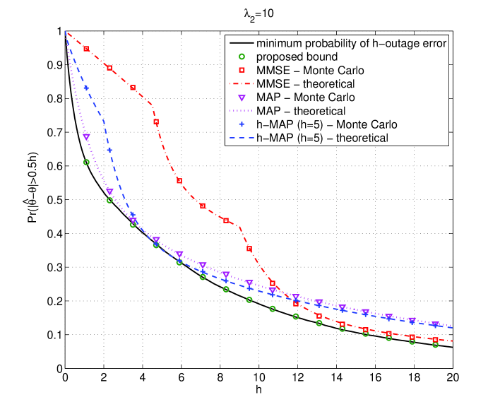
Figure 1: Probability of error versus $h$ for $\lambda_{2}=10$ and unimodal non-symmetric exponential pdf.

Fig. 2 shows the $h$-outage error probability with $h=20$ obtained by MMSE, MAP, and $h$-MAP ($h=20$) estimators compared to the proposed bound versus $\frac{1}{\lambda_{2}}$. This figure shows that the lower bound on the $h$-outage error probability with $h=20$ coincides with the performance of the corresponding $h$-MAP ($h=20$) estimator.

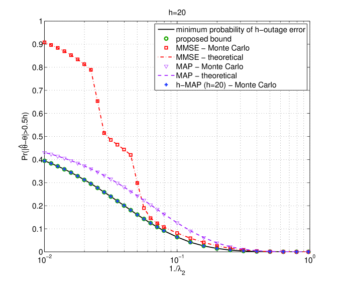
Figure 2: Probability of $h$-outage error for $h=20$ as a function of $\frac{1}{\lambda_{2}}$ for unimodal non-symmetric exponential pdf.

VII-C Example 3

Consider the following observation model

$$x=\theta+w$$ (52)

where the unknown parameter, $\theta$, is distributed according to

$$f_{\theta}(\varphi)=\frac{1}{6}\left(u(\varphi-3)-u(\varphi-6)+u(\varphi+6)-u(\varphi+3)\right)\;,$$

$w$ is a zero-mean Gaussian random variable with known variance $\sigma^{2}$, and $\theta$ and $w$ are statistically independent.

The $h$-MAP estimator for this problem is

$$\hat{\theta}_{h{\text{-}}MAP}=\left\{\begin{array}[]{cc}\left(6-\frac{h}{2}\right)sgn(x)&|x|>6-\frac{h}{2}\text{ or }g(h)<|x|<1.5,6<h\leq 9\\ \left(3+\frac{h}{2}\right)sgn(x)&|x|<3+\frac{h}{2},h\leq 6\\ 0&h\geq 12\\ x&\text{otherwise}\end{array}\right.\;$$ (53)

where $g(h)$ is the solution of $2erf\left(\frac{h}{2\sqrt{2\sigma^{2}}}\right)=erf\left(\frac{g(h)+3}{\sqrt{2\sigma^{2}}}\right)-erf\left(\frac{g(h)-6}{\sqrt{2\sigma^{2}}}\right)$ and $sgn(\cdot)$ it the sign function. The corresponding minimum probability of $h$-outage error is

$$\min_{\hat{\theta}({\bf{x}})}Pr\left(\left|\hat{\theta}-\theta\right|>\frac{h}{2}\right)=\hskip 312.9803pt$$

$$\left\{\begin{array}[]{lc}\frac{1}{6}\left(b(h)-(3+h)erf\left(\frac{3+h}{\sqrt{2\sigma^{2}}}\right)+3erf\left(\frac{3}{\sqrt{2\sigma^{2}}}\right)+\sqrt{\frac{2\sigma^{2}}{\pi}}\left(e^{-\frac{9}{2\sigma^{2}}}-e^{-\frac{\left(3+h\right)^{2}}{2\sigma^{2}}}\right)\right)&0\leq h<3\\ \frac{1}{6}\left(3-6erf\left(\frac{6}{\sqrt{2\sigma^{2}}}\right)+3erf\left(\frac{3}{\sqrt{2\sigma^{2}}}\right)+\sqrt{\frac{2\sigma^{2}}{\pi}}\left(e^{-\frac{9}{2\sigma^{2}}}-e^{-\frac{36}{2\sigma^{2}}}\right)\right)&3\leq h<6\\ \frac{1}{6}\left(3+3erf\left(\frac{g(h)+3}{\sqrt{2\sigma^{2}}}\right)-6erf\left(\frac{6-g(h)}{\sqrt{2\sigma^{2}}}\right)+\sqrt{\frac{2\sigma^{2}}{\pi}}\left(e^{-\frac{\left(g(h)+3\right)^{2}}{2\sigma^{2}}}-e^{-\frac{\left(6-g(h)\right)^{2}}{2\sigma^{2}}}\right)\right)&6\leq h<9\\ \frac{12-h}{6}\left(1-erf\left(\frac{h}{2\sqrt{2\sigma^{2}}}\right)\right)&9\leq h<12\\ 0&h\geq 12\end{array}\right.\;,$$ (59)

where $b(h)\stackrel{{\scriptstyle\triangle}}{{=}}6-h-(6-2h)erf\left(\frac{h}{2\sqrt{2\sigma^{2}}}\right)$. It should be noticed that the $h$-MAP estimator is not unique for $h>3$. In addition, there is no single estimator that attains the minimum probability of $h$-outage error for every $h$. The MAP estimator is obtained by (53) in the limit $h\rightarrow 0$, that is

$$\hat{\theta}_{MAP}=\left\{\begin{array}[]{cc}6sign(x)&|x|>6\\ x&3\leq|x|\leq 6\\ 3sign(x)&|x|<3\end{array}\right.\;,$$

and the MMSE estimator in this case is

$$\hat{\theta}_{MMSE}=x+\frac{1}{c(x)}\sqrt{\frac{2\sigma^{2}}{\pi}}\left(e^{-\frac{\left(x+6\right)^{2}}{2\sigma^{2}}}-e^{-\frac{\left(x+3\right)^{2}}{2\sigma^{2}}}-e^{-\frac{\left(x-6\right)^{2}}{2\sigma^{2}}}+e^{-\frac{\left(x-3\right)^{2}}{2\sigma^{2}}}\right)$$

where $c(x)=erf\left(\frac{x+6}{\sqrt{2\sigma^{2}}}\right)-erf\left(\frac{x-6}{\sqrt{2\sigma^{2}}}\right)+erf\left(\frac{x-3}{\sqrt{2\sigma^{2}}}\right)-erf\left(\frac{x+3}{\sqrt{2\sigma^{2}}}\right)$. Using (33) and the “valley-filling” operator, the proposed bound on the outage error probability in this case is

$$B_{\frac{h}{2},1}^{(o)}=\left\{\begin{array}[]{cc}\frac{1}{6}\left(b(h)-herf\left(\frac{\frac{h}{2}+3}{\sqrt{2\sigma^{2}}}\right)\right)&0\leq h<3\\ \frac{1}{2}\left(1-erf\left(\frac{9}{2\sqrt{2\sigma^{2}}}\right)\right)&3\leq h<9\\ \frac{12-h}{6}\left(1-erf\left(\frac{h}{2\sqrt{2\sigma^{2}}}\right)\right)&9\leq h<12\\ 0&h\geq 12\end{array}\right.$$ (64)

The Ziv-Zakai probability of outage error lower bound (defined in Appendix D) for this problem is

$$I_{ZZLB}(h)=\left\{\begin{array}[]{cc}\frac{1}{6}\max\left(b(h)-h,3-3erf\left(\frac{9}{2\sqrt{2\sigma^{2}}}\right)\right)&0\leq h<3\\ \frac{1}{2}\left(1-erf\left(\frac{9}{2\sqrt{2\sigma^{2}}}\right)\right)&3\leq h<9\\ \frac{12-h}{6}\left(1-erf\left(\frac{h}{2\sqrt{2\sigma^{2}}}\right)\right)&9\leq h<12\\ 0&h\geq 12\;.\end{array}\right.$$ (65)

The minimum $h$-outage error probability, the proposed tightest bound, and the ZZLB on the probability of outage error are presented in Fig. 3 as a function of $h$ for $\sigma^{2}=100$. In addition, the outage error probabilities of the MMSE, MAP, and $h$-MAP ($h=1.5$) estimators are presented in this figure. It can be seen that the proposed bound approaches the minimum outage error probability for every $h$ and for $h<3$ there is a significant difference between the proposed bound and the outage error probability used in the ZZLB expression.

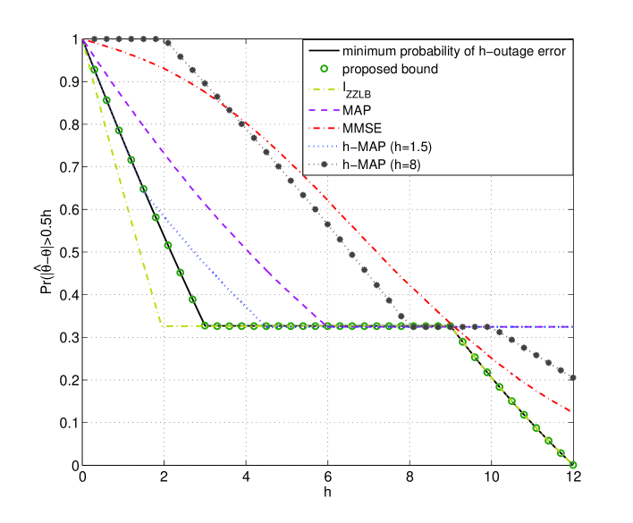
Figure 3: Probability of error versus $h$ for linear non-Gaussian model with $\sigma^{2}=100$.

VIII Conclusion

In this paper, new classes of lower bounds on the probability of outage error and on the MSE in Bayesian parameter estimation were presented. The tightest subclasses of lower bounds in the proposed classes have been derived and the tightest bounds in these subclasses are presented. For unimodal conditional pdf the tightest outage error probability lower bound provides the minimum attainable probability of outage error. For unimodal and symmetric conditional pdf the tightest proposed MSE bound provides the minimum attainable MSE. It is proved that the proposed MSE bound is always tighter than the well known ZZLB. The applicability of the proposed bounds was shown via examples.

Appendix A. Proof of Theorem 1

Sufficient condition: Let $g_{h}({\bf{x}},\theta)$ be periodic in $\theta$ with period $h$, for almost every ${\bf{x}}\in\chi$. In particular,

$$\int_{\hat{\theta}-\frac{h}{2}}^{\hat{\theta}+\frac{h}{2}}g_{h}({\bf{x}},\varphi){\,\mathrm{d}}\varphi=c({\bf{x}},h),~{}~{}~{}\forall\hat{\theta}$$ (66)

where $c({\bf{x}},h)$ is not a function of the estimator $\hat{\theta}$. Thus, using (7) and (9)

$${\rm E}\left[\left|u_{h}({\bf{x}},\theta)v_{h}\left({\bf{x}},\theta\right)\right|\right]={\rm E}\left[\int_{\hat{\theta}-\frac{h}{2}}^{\hat{\theta}+\frac{h}{2}}g_{h}({\bf{x}},\varphi){\,\mathrm{d}}\varphi\right]={\rm E}\left[c({\bf{x}},h)\right]$$ (67)

is independent of the estimator $\hat{\theta}$.

Necessary condition: Let ${\rm E}\left[\left|u_{h}({\bf{x}},\theta)v_{h}\left({\bf{x}},\theta\right)\right|\right]$ be independent of the estimator $\hat{\theta}$ and define the following family of estimators

$$\hat{\theta}_{A,\alpha}({\bf{x}})=\alpha_{A}{\mathbf{1}}_{{\bf{x}}\in A}$$ (68)

where ${\bf{x}}$ is a random observation vector, the indicator function, ${\mathbf{1}}_{{\bf{x}}\in A}$, is defined as

$${\mathbf{1}}_{{\bf{x}}\in A}=\left\{\begin{array}[]{cc}\alpha_{A}&\text{if }{\bf{x}}\in A\\ 0&\text{if }{\bf{x}}\in A^{c}\end{array}\right.,~{}~{}~{}\alpha_{A}\in{\mathbb{R}}\;,$$

and $A^{c}$ is the complementary event of $A$. Then, under the assumption that ${\rm E}\left[\left|u_{h}({\bf{x}},\theta)v_{h}\left({\bf{x}},\theta\right)\right|\right]$ is independent of the estimator $\hat{\theta}$, in particular, for each estimator $\hat{\theta}_{A,\alpha}({\bf{x}})$

$${\rm E}\left[\left|u_{h}({\bf{x}},\theta)v_{h}\left({\bf{x}},\theta\right)\right|\right] = {\rm E}\left[\int_{\hat{\theta}_{A,\alpha}({\bf{x}})-\frac{h}{2}}^{\hat{\theta}_{A,\alpha}({\bf{x}})+\frac{h}{2}}g_{h}({\bf{x}},\varphi){\,\mathrm{d}}\varphi\right]$$ (69)

$$= {\rm E}\left[{\mathbf{1}}_{{\bf{x}}\in A^{c}}\int_{-\frac{h}{2}}^{\frac{h}{2}}g_{h}({\bf{x}},\varphi){\,\mathrm{d}}\varphi\right]+{\rm E}\left[{\mathbf{1}}_{{\bf{x}}\in A}\int_{\alpha_{A}-\frac{h}{2}}^{\alpha_{A}+\frac{h}{2}}g_{h}({\bf{x}},\varphi){\,\mathrm{d}}\varphi\right]$$

$$= {\rm E}\left[\int_{-\frac{h}{2}}^{\frac{h}{2}}g_{h}({\bf{x}},\varphi){\,\mathrm{d}}\varphi\right]+{\rm E}\left[{\mathbf{1}}_{{\bf{x}}\in A}\left(\int_{\alpha_{A}-\frac{h}{2}}^{\alpha_{A}+\frac{h}{2}}g_{h}({\bf{x}},\varphi){\,\mathrm{d}}\varphi-\int_{-\frac{h}{2}}^{\frac{h}{2}}g_{h}({\bf{x}},\varphi){\,\mathrm{d}}\varphi\right)\right]$$

is independent of $A$ or $\alpha_{A}$. Thus, ${\rm E}\left[{\mathbf{1}}_{{\bf{x}}\in A}\left(\int_{\alpha_{A}-\frac{h}{2}}^{\alpha_{A}+\frac{h}{2}}g_{h}({\bf{x}},\varphi){\,\mathrm{d}}\varphi-\int_{-\frac{h}{2}}^{\frac{h}{2}}g_{h}({\bf{x}},\varphi){\,\mathrm{d}}\varphi\right)\right]$ is identical for every $A$ and $\alpha_{A}$. In particular, by setting $A=\emptyset$ where $\emptyset$ is the empty set, one obtains
${\rm E}\left[{\mathbf{1}}_{{\bf{x}}\in\emptyset}\left(\int_{\alpha_{\emptyset}-\frac{h}{2}}^{\alpha_{\emptyset}+\frac{h}{2}}g_{h}({\bf{x}},\varphi){\,\mathrm{d}}\varphi-\int_{-\frac{h}{2}}^{\frac{h}{2}}g_{h}({\bf{x}},\varphi){\,\mathrm{d}}\varphi\right)\right]=0$, and therefore
${\rm E}\left[{\mathbf{1}}_{{\bf{x}}\in A}\left(\int_{\alpha_{A}-\frac{h}{2}}^{\alpha_{A}+\frac{h}{2}}g_{h}({\bf{x}},\varphi){\,\mathrm{d}}\varphi-\int_{-\frac{h}{2}}^{\frac{h}{2}}g_{h}({\bf{x}},\varphi){\,\mathrm{d}}\varphi\right)\right]=0$ for every $A$. Accordingly,

$$\int_{\alpha_{A}-\frac{h}{2}}^{\alpha_{A}+\frac{h}{2}}g_{h}({\bf{x}},\varphi){\,\mathrm{d}}\varphi-\int_{-\frac{h}{2}}^{\frac{h}{2}}g_{h}({\bf{x}},\varphi){\,\mathrm{d}}\varphi=0,~{}~{}~{}a.e.~{}{\bf{x}}\in\chi,~{}\forall\alpha_{A}\in{\mathbb{R}}\;.$$ (70)

Equation (70) indicates that under the assumption that $f_{\theta|{\bf{x}}}(\varphi|{\bf{x}})>0,~{}~{}~{}\forall{\bf{x}}\in\chi,~{}\varphi\in\mathbb{R}$, the term ${\rm E}\left[\int_{\hat{\theta}-\frac{h}{2}}^{\hat{\theta}+\frac{h}{2}}g_{h}({\bf{x}},\varphi){\,\mathrm{d}}\varphi\right]$ is independent of the estimator $\hat{\theta}$ only if $g_{h}({\bf{x}},\theta)$ is a periodic function w.r.t. $\theta$ with period $h$ for a.e. ${\bf{x}}\in\chi$.

Appendix B. Eq. (25) yields a global maximum of the bound in (24)

In this appendix, it is shown that the stationary point of (24) w.r.t. the Fourier coefficients $\left\{a_{k}({\bf{x}},h)\right\}$ is a global maximum, that is, it will be shown that the Hessian matrix of (24) w.r.t. the coefficients $\{a_{k}({\bf{x}},h)\}_{k\in{\mathbb{Z}},k\neq 0}$ is a negative-definite matrix at the point $\{a_{k}^{(o)}({\bf{x}},h)\}_{k\in{\mathbb{Z}},k\neq 0}$ which satisfies (25). The derivation in this appendix is carried out under the assumption that ${\bf{x}}$ is a continuous random vector. Extension to any random vector ${\bf{x}}$ satisfying $||{\bf{x}}||_{2}^{2}<\infty$ is straightforward. For example, if ${\bf{x}}$ is a discrete random vector with the probabilities $P({\bf{x}}={\bf{x}}_{i})=p_{i},~{}i=0,1,\ldots$, the pdf $f_{\bf{x}}({\bf{x}}_{0})$ is replaced by $p_{0}$ along the proof.

Under the assumption that the integration and derivatives can be reordered, the derivatives of (24) w.r.t. $\left\{a_{m}({\bf{x}}_{0},h)\right\},~{}~{}~{}\forall m\in{\mathbb{Z}},~{}m\neq 0,~{}{\bf{x}}_{0}\in\chi$ are

$$\frac{\partial B_{\frac{h}{2},p}}{\partial a_{m}({\bf{x}}_{0},h)}=\frac{1}{p}h^{\frac{1}{p}}a_{0}^{\frac{1}{p}}({\bf{x}}_{0},h)f_{\bf{x}}({\bf{x}}_{0})\left(\int\limits_{{\mathbb{R}}}\left(\sum_{k=-\infty}^{\infty}a_{k}({\bf{x}},h)e^{i\frac{2\pi k}{h}\varphi}\right)^{\frac{1}{1-p}}f_{\theta|{\bf{x}}}^{\frac{p}{p-1}}(\varphi|{\bf{x}}){\,\mathrm{d}}\varphi\right)^{\frac{-1}{p}}\times$$

$$\int_{{\mathbb{R}}}\left(\sum_{k=-\infty}^{\infty}a_{k}({\bf{x}}_{0},h)e^{i\frac{2\pi k}{h}\varphi}\right)^{\frac{p}{1-p}}f_{\theta|{\bf{x}}}^{\frac{p}{p-1}}(\varphi|{\bf{x}}_{0})e^{i\frac{2\pi m}{h}\varphi}{\,\mathrm{d}}\varphi,$$ (71)

and by equating (Appendix B. Eq. (25) yields a global maximum of the bound in (24)) to zero (note that $\int\limits_{{\mathbb{R}}}\left(\sum_{k=-\infty}^{\infty}a_{k}({\bf{x}},h)e^{i\frac{2\pi k}{h}\varphi}\right)^{\frac{1}{1-p}}f_{\theta|{\bf{x}}}^{\frac{p}{p-1}}(\varphi|{\bf{x}}){\,\mathrm{d}}\varphi>0$ according to H$\ddot{\text{o}}$lder’s inequality properties), one obtains

$$\int_{{\mathbb{R}}}\left(\sum_{k=-\infty}^{\infty}a_{k}^{(0)}({\bf{x}}_{0},h)e^{i\frac{2\pi k}{h}\varphi}\right)^{\frac{p}{1-p}}f_{\theta|{\bf{x}}}^{\frac{p}{p-1}}(\varphi|{\bf{x}}_{0})e^{i\frac{2\pi m}{h}\varphi}{\,\mathrm{d}}\varphi=0,~{}~{}~{}\forall m\in{\mathbb{Z}},~{}m\neq 0,~{}{\bf{x}}_{0}\in\chi\;.$$ (72)

The second order derivatives are obtained as follows

$$[{\bf{H}}]_{m,l}=\frac{\partial^{2}B_{\frac{h}{2},p}}{\partial a_{m}({\bf{x}}_{0},h)\partial a_{-l}({\bf{x}}_{0},h)}\hskip 341.43306pt$$

$$=\frac{1}{p^{2}(p-1)}h^{\frac{1}{p}}a_{0}^{\frac{1}{p}}({\bf{x}}_{0},h)f_{\bf{x}}({\bf{x}}_{0})\left(\int\limits_{{\mathbb{R}}}\left(\sum_{k=-\infty}^{\infty}a_{k}({\bf{x}},h)e^{i\frac{2\pi k}{h}\varphi}\right)^{\frac{1}{1-p}}f_{\theta|{\bf{x}}}^{\frac{p}{p-1}}(\varphi|{\bf{x}}){\,\mathrm{d}}\varphi\right)^{\frac{-1-p}{p}}\times\hskip 56.9055pt$$

$$\int_{{\mathbb{R}}}\left(\sum_{k=-\infty}^{\infty}a_{k}({\bf{x}}_{0},h)e^{i\frac{2\pi k}{h}\varphi}\right)^{\frac{p}{1-p}}f_{\theta|{\bf{x}}}^{\frac{p}{p-1}}(\varphi|{\bf{x}}_{0})e^{i\frac{2\pi m}{h}\varphi}{\,\mathrm{d}}\varphi\int_{{\mathbb{R}}}\left(\sum_{k=-\infty}^{\infty}a_{k}({\bf{x}}_{0},h)e^{i\frac{2\pi k}{h}\varphi}\right)^{\frac{p}{1-p}}f_{\theta|{\bf{x}}}^{\frac{p}{p-1}}(\varphi|{\bf{x}}_{0})e^{-i\frac{2\pi l}{h}\varphi}{\,\mathrm{d}}\varphi$$

$$-\frac{1}{p-1}h^{\frac{1}{p}}a_{0}^{\frac{1}{p}}({\bf{x}}_{0},h)f_{\bf{x}}({\bf{x}}_{0})\left(\int\limits_{{\mathbb{R}}}\left(\sum_{k=-\infty}^{\infty}a_{k}({\bf{x}},h)e^{i\frac{2\pi k}{h}\varphi}\right)^{\frac{1}{1-p}}f_{\theta|{\bf{x}}}^{\frac{p}{p-1}}(\varphi|{\bf{x}}){\,\mathrm{d}}\varphi\right)^{\frac{-1}{p}}\times\hskip 85.35826pt$$

$$\int_{{\mathbb{R}}}\left(\sum_{k=-\infty}^{\infty}a_{k}({\bf{x}}_{0},h)e^{i\frac{2\pi k}{h}\varphi}\right)^{\frac{2p-1}{1-p}}f_{\theta|{\bf{x}}}^{\frac{p}{p-1}}(\varphi|{\bf{x}}_{0})e^{i\frac{2\pi(m-l)}{h}\varphi}{\,\mathrm{d}}\varphi\hskip 170.71652pt$$ (73)

for all $m,l\in{\mathbb{Z}},~{}m,l\neq 0,~{}{\bf{x}}_{0}\in\chi$, where ${\bf{H}}$ is the Hessian matrix. By substituting (72) in (Appendix B. Eq. (25) yields a global maximum of the bound in (24)), the Hessian matrix at $\{a_{k}^{(o)}({\bf{x}}_{0},h)\}$ is

$$\left[{\bf{H}}\left(\left\{a_{k}^{(o)}({\bf{x}}_{0},h)\right\}\right)\right]_{m,l}=-c_{1}({\bf{x}}_{0},h)\int_{{\mathbb{R}}}c_{2}({\bf{x}}_{0},\varphi,h)[{\bf{F}}]_{m,l}(\varphi){\,\mathrm{d}}\varphi,$$ (74)

where

$$c_{1}({\bf{x}}_{0},h)\stackrel{{\scriptstyle\triangle}}{{=}}h^{\frac{1}{p}}a_{0}^{\frac{1}{p}}({\bf{x}}_{0},h)\frac{1}{p-1}f_{\bf{x}}({\bf{x}}_{0})\left(\int\limits_{{\mathbb{R}}}\left(\sum_{k=-\infty}^{\infty}a_{k}({\bf{x}},h)e^{i\frac{2\pi k}{h}\varphi}\right)^{\frac{1}{1-p}}f_{\theta|{\bf{x}}}^{\frac{p}{p-1}}(\varphi|{\bf{x}}){\,\mathrm{d}}\varphi\right)^{\frac{-1}{p}}\;,$$

$$c_{2}({\bf{x}}_{0},\varphi,h)\stackrel{{\scriptstyle\triangle}}{{=}}\left(\sum_{k=-\infty}^{\infty}a_{k}^{(o)}({\bf{x}}_{0},h)e^{i\frac{2\pi k}{h}\varphi}\right)^{\frac{2p-1}{1-p}}f_{\theta|{\bf{x}}}^{\frac{p}{p-1}}(\varphi|{\bf{x}}_{0}),$$

and $[{\bf{F}}]_{m,l}(\varphi)=e^{i\frac{2\pi(m-l)}{h}\varphi}$ is the $m,l$th Fourier coefficient for any period $h$ and for all $\varphi\in{\mathbb{R}}$. The periodic function, $\sum_{k=-\infty}^{\infty}a_{k}^{(o)}({\bf{x}}_{0},h)e^{i\frac{2\pi k}{h}\varphi}$, is positive for almost all $\varphi\in{\mathbb{R}}$ and ${\bf{x}}_{0}\in\chi$ and in particular $a_{0}({\bf{x}}_{0},h)>0$ (according to (10) $\{a_{k}({\bf{x}},h)\}$ should be chosen such that $\sum_{k=-\infty}^{\infty}a_{k}({\bf{x}}_{0},h)e^{i\frac{2\pi k}{h}\varphi}$ is a positive function) and thus $c_{1}({\bf{x}}_{0},h)>0$ and $c_{2}({\bf{x}}_{0},\varphi,h)>0$ for all $h>0$, $p>0$ and for almost all $\varphi\in{\mathbb{R}}$ and ${\bf{x}}_{0}\in\chi$. For given $\varphi\in{\mathbb{R}}$, the infinite matrix of the Fourier coefficients, ${\bf{F}}(\varphi)$, is known to be positive-definite. Therefore, ${\bf{H}}$ is an infinite positive-definite matrix and (72) yields a maximum of (24).

Appendix C. Unknown parameter with bounded support

The derivations in Sections III and IV are carried out under the assumption that the unknown parameter is unbounded with $f_{\theta|{\bf{x}}}(\theta|{\bf{x}})>0,~{}~{}~{}\forall\theta\in{\mathbb{R}}$ for almost all ${\bf{x}}\in\chi$. In this appendix, it is shown that the derived bounds are suitable also for parameters with any support. The support of the unknown parameter $\theta$ for given observation vector, ${\bf{x}}$, is defined as

$$S_{\theta|{\bf{x}}}=\overline{\left\{\varphi:f_{\theta|{\bf{x}}}(\varphi|{\bf{x}})>0,~{}\varphi\in{\mathbb{R}}\right\}}$$

where $\overline{A}$ is the closure of a set $A$.

Let define the function

$$\varepsilon({\bf{x}},\theta)=\left\{\begin{array}[]{lr}0&\text{if }\theta\in S_{\theta|{\bf{x}}}\\ \delta\frac{1}{\sqrt{2\pi\sigma^{2}}}e^{-\frac{-\theta^{2}}{2\sigma^{2}}}&\text{if }\theta\notin S_{\theta|{\bf{x}}}\end{array}\right.$$ (75)

where $\delta>0$, $\sigma\gg 1$. Using this definition, it can be stated that

$${\rm E}\left[\left|v_{h}({\bf{x}},\theta)\right|^{\frac{1}{1-p}}\right]={\rm E}\left[\int_{S_{\theta|{\bf{x}}}}f_{\theta|{\bf{x}}}(\varphi|{\bf{x}})\left|v_{h}({\bf{x}},\varphi)\right|^{\frac{1}{1-p}}{\,\mathrm{d}}\varphi\right]={\rm E}\left[\int_{S_{\theta|{\bf{x}}}}\left(f_{\theta|{\bf{x}}}(\varphi|{\bf{x}})+\varepsilon({\bf{x}},\varphi)\right)\left|v_{h}({\bf{x}},\varphi)\right|^{\frac{1}{1-p}}{\,\mathrm{d}}\varphi\right]$$ (76)

and

$${\rm E}^{\frac{1}{p}}\left[\int_{\hat{\theta}-\frac{h}{2}}^{{\hat{\theta}+\frac{h}{2}}}f_{\theta|{\bf{x}}}(\varphi|{\bf{x}})\left|v_{h}\left({\bf{x}},\varphi\right)\right|{\,\mathrm{d}}\varphi\right]\leq{\rm E}^{\frac{1}{p}}\left[\int_{\hat{\theta}-\frac{h}{2}}^{{\hat{\theta}+\frac{h}{2}}}\left(f_{\theta|{\bf{x}}}(\varphi|{\bf{x}})+\varepsilon({\bf{x}},\varphi)\right)\left|v_{h}\left({\bf{x}},\varphi\right)\right|{\,\mathrm{d}}\varphi\right],~{}p>1\;.$$ (77)

Using (8), (76), and (77), one obtains the following lower bound on the outage error probability

$$Pr\left(\left|\hat{\theta}-\theta\right|>\frac{h}{2}\right)\hskip 369.88582pt$$

$$\geq 1-{\rm E}^{\frac{1}{p}}\left[\int_{\hat{\theta}-\frac{h}{2}}^{{\hat{\theta}+\frac{h}{2}}}(f_{\theta|{\bf{x}}}(\varphi|{\bf{x}})+\varepsilon({\bf{x}},\varphi))\left|v_{h}\left({\bf{x}},\varphi\right)\right|{\,\mathrm{d}}\varphi\right]{\rm E}^{\frac{p-1}{p}}\left[\int_{S_{\theta|{\bf{x}}}}(f_{\theta|{\bf{x}}}(\varphi|{\bf{x}})+\varepsilon({\bf{x}},\varphi))\left|v_{h}({\bf{x}},\theta)\right|^{\frac{1}{1-p}}\right],$$ (78)

for all $\delta>0$, $p>1$. In similar to Theorem 1, define the function

$$\tilde{g}_{h}({\bf{x}},\theta)\stackrel{{\scriptstyle\triangle}}{{=}}\left(f_{\theta|{\bf{x}}}(\theta|{\bf{x}})+\varepsilon({\bf{x}},\theta)\right)|v_{h}({\bf{x}},\theta)|\;.$$ (79)

A valid bound which is independent on $\hat{\theta}$ is obtained iff $\tilde{g}_{h}({\bf{x}},\theta)$ is periodic in $\theta$ with period $h$, for a.e. ${\bf{x}}\in\chi$ and $\theta\in{\mathbb{R}}$ and the periodic extension $\tilde{g}_{h}({\bf{x}},\theta)$ can be represented using Fourier series [18]:

$$\tilde{g}_{h}({\bf{x}},\theta)=\sum_{k=-\infty}^{\infty}b_{k}({\bf{x}},h)e^{i\frac{2\pi k}{h}\theta},~{}~{}a.e.~{}{\bf{x}}\in\chi\;.$$ (80)

The derivation in Section III is valid for bounded support where $g_{h}({\bf{x}},\theta)$ is replaced by $\tilde{g}_{h}({\bf{x}},\theta)$. The general class of lower bounds on the probability of error in the bounded support parameter estimation problem is

$$\tilde{B}_{\frac{h}{2},p} = 1-h^{\frac{1}{p}}{\rm E}^{\frac{1}{p}}\left[b_{0}({\bf{x}},h)\right]{\rm E}^{\frac{p-1}{p}}\left[\int\limits_{-\infty}^{\infty}\left(\sum_{k=-\infty}^{\infty}b_{k}({\bf{x}},h)e^{i\frac{2\pi k}{h}\varphi}\right)^{\frac{1}{1-p}}\left(f_{\theta|{\bf{x}}}(\varphi|{\bf{x}})+\varepsilon({\bf{x}},\varphi)\right)^{\frac{p}{p-1}}{\,\mathrm{d}}\varphi\right],$$ (81)

for all $p>1$ and $h>0$. The tightest subclass of bounds in this class is given by $Pr\left(\left|\hat{\theta}-\theta\right|>\frac{h}{2}\right)\geq\tilde{B}_{\frac{h}{2},p}^{(o)}$, $p>1,$ where

$$\tilde{B}_{\frac{h}{2},p}^{(o)}=1-{\rm E}\left[\int_{0}^{h}\left(\sum_{l=-\infty}^{\infty}\left(f_{\theta|{\bf{x}}}(\varphi+lh|{\bf{x}})+\varepsilon({\bf{x}},\varphi+lh)\right)^{\frac{p}{p-1}}\right)^{\frac{p-1}{p}}{\,\mathrm{d}}\varphi\right]\;.$$ (82)

Using (75) and taking the limit $\delta\rightarrow 0$ in (81) and (82), yields the bounds

$$\tilde{B}_{\frac{h}{2},p} = 1-h^{\frac{1}{p}}{\rm E}^{\frac{1}{p}}\left[b_{0}({\bf{x}},h)\right]{\rm E}^{\frac{p-1}{p}}\left[\int\limits_{-\infty}^{\infty}\left(\sum_{k=-\infty}^{\infty}b_{k}({\bf{x}},h)e^{i\frac{2\pi k}{h}\varphi}\right)^{\frac{1}{1-p}}\left(f_{\theta|{\bf{x}}}(\varphi|{\bf{x}})\right)^{\frac{p}{p-1}}{\,\mathrm{d}}\varphi\right],~{}~{}~{}p>1,$$ (83)

and

$$\tilde{B}_{\frac{h}{2},p}^{(o)}=1-{\rm E}\left[\int_{0}^{h}\left(\sum_{l=-\infty}^{\infty}f_{\theta|{\bf{x}}}^{\frac{p}{p-1}}(\varphi+lh|{\bf{x}})\right)^{\frac{p-1}{p}}{\,\mathrm{d}}\varphi\right],~{}~{}~{}p>1\;,$$ (84)

respectively. In particular, for $p\rightarrow 1^{+}$, the bound in (84) becomes

$$\tilde{B}_{\frac{h}{2},1}^{(o)}=1-{\rm E}\left[\int_{0}^{h}\max_{l\in\mathbb{Z}}\left\{f_{\theta|{\bf{x}}}(\varphi+lh|{\bf{x}})\right\}{\,\mathrm{d}}\varphi\right]$$ (85)

which is the tightest bound on the outage error probability in the proposed class of lower bounds. Accordingly, the proposed bounds can be applied to any parameter estimation problem with unknown continuous random variable.

Appendix D. The proposed MSE bound is tighter than the ZZLB

In this appendix, it is analytically shown that the proposed MSE bound in (41) is always tighter than the ZZLB. For the sake of simplicity, we will assume that ${\bf{x}}$ is continuous random variable. Extension to any random vector ${\bf{x}}$ satisfying $||{\bf{x}}||_{2}^{2}<\infty$ is straightforward. The MSE lower bound from (41) can be rewritten as

$${C_{1}^{(o)}}=\frac{1}{2}\int\limits_{0}^{\infty}{\rm E}\left[\int\limits_{-\infty}^{\infty}f_{\theta|{\bf{x}}}(\varphi|{\bf{x}}){\,\mathrm{d}}\varphi-\int\limits_{0}^{h}\max_{l\in\mathbb{Z}}f_{\theta|{\bf{x}}}(\varphi+lh|{\bf{x}}){\,\mathrm{d}}\varphi\right]h{\,\mathrm{d}}h\;.$$ (86)

Using the convergence condition in (26), the first integral in (86) can be divided into infinite sum of integrals, where each integral is over a single period and (86) can be rewritten as

$$C_{1}^{(o)}=\frac{1}{2}\int\limits_{0}^{\infty}{\rm E}\left[\int\limits_{0}^{h}\min_{l\in\mathbb{Z}}\sum_{\stackrel{{\scriptstyle k=-\infty}}{{k\neq l}}}^{\infty}f_{\theta|{\bf{x}}}(\varphi+kh|{\bf{x}}){\,\mathrm{d}}\varphi\right]h{\,\mathrm{d}}h\;.$$ (87)

The ZZLB (without the valley-filling function) is [7]

$$B_{ZZLB}=\frac{1}{2}\int\limits_{0}^{\infty}\left(\int\limits_{-\infty}^{\infty}\left(f_{\theta}(\varphi)+f_{\theta}(\varphi+h)\right)P_{min}(\varphi,\varphi+h){\,\mathrm{d}}\varphi\right)h{\,\mathrm{d}}h$$ (88)

where $f_{\theta}(\cdot)$ is the a-priori pdf of $\theta$ and $P_{min}(\varphi,\varphi+h)$ is the minimum probability of error for the following detection problem:

$${\begin{array}[]{rl}&H_{0}:f_{{\bf{x}}|H_{0}}({\bf{x}})=f_{{\bf{x}}|\theta}({\bf{x}}|\varphi)\\ &H_{1}:f_{{\bf{x}}|H_{1}}({\bf{x}})=f_{{\bf{x}}|\theta}({\bf{x}}|\varphi+h)\end{array}}$$ (89)

where $f_{{\bf{x}}|H_{i}}(\cdot),~{}i=1,2$ is the pdf of the observation vector ${\bf{x}}$ under each hypothesis, and the prior probabilities are

$$P(H_{0})=\frac{f_{\theta}(\varphi)}{f_{\theta}(\varphi)+f_{\theta}(\varphi+h)},~{}~{}~{}P(H_{1})=1-P(H_{0})\;.$$ (90)

It is well known that the minimum probability of error is obtained by the MAP criterion and for binary hypothesis testing it is given by [21]

$$P_{min}(\varphi,\varphi+h)=1-{\rm E}\left[\max_{i=1,2}P(H_{i}|{\bf{x}})\right]={\rm E}\left[\min_{i=1,2}P(H_{i}|{\bf{x}})\right]\;.$$ (91)

By substituting (89) - (90) in (91), the minimum probability of error obtained by the MAP detector is

$$P_{min}(\varphi,\varphi+h)={\rm E}\left[\min\left(\frac{f_{{\bf{x}}|\theta}({\bf{x}}|\varphi)f_{\theta}(\varphi)}{\left(f_{\theta}(\varphi)+f_{\theta}(\varphi+h)\right)},\frac{f_{{\bf{x}}|\theta}({\bf{x}}|\varphi+h)f_{\theta}(\varphi+h)}{f_{\bf{x}}({\bf{x}})\left(f_{\theta}(\varphi)+f_{\theta}(\varphi+h)\right)}\right)\right]\;.$$ (92)

Note that since ${\bf{x}}$ is the only random variable in (92), the expectation is performed w.r.t. ${\bf{x}}$. By substituting (92) in (88), one obtains

$$B_{ZZLB} = \frac{1}{2}\int\limits_{0}^{\infty}\int\limits_{-\infty}^{\infty}{\rm E}\left[\min\left(\frac{f_{{\bf{x}}|\theta}({\bf{x}}|\varphi)f_{\theta}(\varphi)}{f_{\bf{x}}({\bf{x}})},\frac{f_{{\bf{x}}|\theta}({\bf{x}}|\varphi+h)f_{\theta}(\varphi+h)}{f_{\bf{x}}({\bf{x}})}\right)\right]{\,\mathrm{d}}\varphi h{\,\mathrm{d}}h$$ (93)

$$= \frac{1}{2}\int\limits_{0}^{\infty}\int\limits_{-\infty}^{\infty}{\rm E}\left[\min\left(f_{\theta|{\bf{x}}}(\varphi|{\bf{x}}),f_{\theta|{\bf{x}}}(\varphi+h|{\bf{x}})\right)\right]{\,\mathrm{d}}\varphi h{\,\mathrm{d}}h\;.$$

Since $\int\limits_{-\infty}^{\infty}{\rm E}\left[\min\left(f_{\theta|{\bf{x}}}(\varphi|{\bf{x}}),f_{\theta|{\bf{x}}}(\varphi+h|{\bf{x}})\right)\right]{\,\mathrm{d}}\varphi\leq\int\limits_{-\infty}^{\infty}{\rm E}\left[f_{\theta|{\bf{x}}}(\varphi|{\bf{x}})\right]{\,\mathrm{d}}\varphi=1$, the inner integral in the r.h.s. of (93) converges (i.e. the ZZLB does not need a convergence condition on the pdf). Therefore, it is possible to change the order of integration w.r.t. ${\bf{x}}$ and $\varphi$, and the integral can be divided into an infinite sum of integrals. Thus,

$$B_{ZZLB} = \frac{1}{2}\int\limits_{0}^{\infty}{\rm E}\left[\int\limits_{-\infty}^{\infty}\min\left(f_{\theta|{\bf{x}}}(\varphi|{\bf{x}}),f_{\theta|{\bf{x}}}(\varphi+h|{\bf{x}})\right){\,\mathrm{d}}\varphi\right]h{\,\mathrm{d}}h$$ (94)

$$= \frac{1}{2}\int\limits_{0}^{\infty}{\rm E}\left[\sum_{l=-\infty}^{\infty}\int_{lh}^{(l+1)h}\min\left(f_{\theta|{\bf{x}}}(\varphi|{\bf{x}}),f_{\theta|{\bf{x}}}\left(\varphi+h|{\bf{x}}\right)\right){\,\mathrm{d}}\varphi\right]h{\,\mathrm{d}}h$$

$$= \frac{1}{2}\int\limits_{0}^{\infty}{\rm{E}}\left[\int\limits_{0}^{h}\sum\limits_{l=-\infty}^{\infty}\min\left(f_{\theta|{\bf{x}}}(\varphi+lh|{\bf{x}}),f_{\theta|{\bf{x}}}(\varphi+(l+1)h|{\bf{x}})\right){\,\mathrm{d}}\varphi\right]h{\,\mathrm{d}}h\;.$$

Thus, the ZZLB can be written as $B_{ZZLB}=\frac{1}{2}\int\limits_{0}^{\infty}I_{ZZLB}(h)h{\,\mathrm{d}}h$ where

$$I_{ZZLB}(h)\stackrel{{\scriptstyle\triangle}}{{=}}V\left\{\int\limits_{-\infty}^{\infty}{\rm E}\left[\min\left(f_{\theta|{\bf{x}}}(\varphi|{\bf{x}}),f_{\theta|{\bf{x}}}(\varphi+h|{\bf{x}})\right)\right]{\,\mathrm{d}}\varphi\right\}$$ (95)

is referred in this paper as the Ziv-Zakai outage error probability lower bound.

In [19] it is shown that $\min\limits_{k}\sum\limits_{n=0,n\neq k}^{M-1}a_{n}\geq\sum\limits_{n=0}^{M-2}\min(a_{n},a_{n+1})$ for any $M$ non-negative numbers $\{a_{n}\}_{n=0}^{M-1}$. In a similar manner, it can be shown that for an infinite countable set of non-negative numbers $\{a_{n}\}_{n\in\mathbb{Z}}$ satisfying $\lim\limits_{n\rightarrow\pm\infty}a_{n}=0$ and $\sum\limits_{n=-\infty}^{\infty}a_{n}<\infty$,

$$\min_{k\in\mathbb{Z}}\sum_{n=-\infty,~{}n\neq k}^{\infty}a_{n}\geq\sum_{n=-\infty}^{\infty}\min(a_{n},a_{n+1})\;.$$

In particular, under the convergence condition in (26)

$$\min_{k\in\mathbb{Z}}\sum_{l=-\infty,l\neq k}^{\infty}f_{\theta|{\bf{x}}}(\varphi+lh|{\bf{x}})\geq\sum\limits_{l=-\infty}^{\infty}\min\left(f_{\theta|{\bf{x}}}(\varphi+lh|{\bf{x}}),f_{\theta|{\bf{x}}}(\varphi+(l+1)h|{\bf{x}})\right)$$ (96)

and thus

$${\rm E}\left[\min_{k\in\mathbb{Z}}\sum_{\stackrel{{\scriptstyle l=-\infty}}{{l\neq k}}}^{\infty}f_{\theta|{\bf{x}}}(\varphi+lh|{\bf{x}})\right]\geq{\rm E}\left[\sum\limits_{l=-\infty}^{\infty}\min\left(f_{\theta|{\bf{x}}}(\varphi+lh|{\bf{x}}),f_{\theta|{\bf{x}}}(\varphi+(l+1)h|{\bf{x}})\right)\right]~{}\;.$$ (97)

Therefore, from (87), (93) and (97), one concludes that

$$C_{1}^{(o)}\geq B_{ZZLB}\;.$$ (98)

Thus, the proposed lower bound in (41) is always tighter than the ZZLB in (88). Applying the valley-filling operator on both sides of (98) does not change this result.

Appendix E. The tightness of the bound for unimodal pdf

In this appendix it is shown that if the conditional pdf $f_{\theta|{\bf{x}}}(\cdot|{\bf{x}})$ is a unimodal function, the outage error probability bound in (33) coincides with the minimum probability of outage error in (1) for every $h>0$. Assume that $f_{\theta|{\bf{x}}}(\cdot|{\bf{x}})$ is unimodal with maximum point $\hat{\theta}_{MAP}({\bf{x}})=\hat{\theta}_{0}({\bf{x}})$. The bound in (33) involves the computation of

$${\rm E}\left[\int_{0}^{h}\max_{l\in\mathbb{Z}}\left\{f_{\theta|{\bf{x}}}\left(\varphi+lh|{\bf{x}}\right)\right\}{\,\mathrm{d}}\varphi\right]={\rm E}\left[\int_{0}^{h}\max_{l\in\mathbb{Z}}\left\{f_{\theta|{\bf{x}}}\left(\hat{\theta}_{0}({\bf{x}})+h\left(l-\frac{\hat{\theta}_{0}({\bf{x}})-\varphi}{h}\right)|{\bf{x}}\right)\right\}{\,\mathrm{d}}\varphi\right]\;.$$ (99)

Since the conditional pdf, $f_{\theta|{\bf{x}}}\left(\cdot|{\bf{x}}\right)$, is unimodal with maximum at $\hat{\theta}_{0}({\bf{x}})$, then

$$\max_{l\in\mathbb{Z}}\left\{f_{\theta|{\bf{x}}}\left(\hat{\theta}_{0}({\bf{x}})+h\left(l-\frac{\hat{\theta}_{0}({\bf{x}})-\varphi}{h}\right)|{\bf{x}}\right)\right\}=\hskip 199.16928pt$$

$$=\max\left\{f_{\theta|{\bf{x}}}\left(\hat{\theta}_{0}({\bf{x}})+ha_{\bf{x}}(\varphi)|{\bf{x}}\right),f_{\theta|{\bf{x}}}\left(\hat{\theta}_{0}({\bf{x}})+h\left(a_{\bf{x}}(\varphi)+1\right)|{\bf{x}}\right)\right\}$$ (100)

for all ${\bf{x}}$ and $\varphi\in(0,h)$ where $a_{\bf{x}}(\varphi)=\left\lfloor\frac{\hat{\theta}_{0}({\bf{x}})-\varphi}{h}\right\rfloor-\frac{\hat{\theta}_{0}({\bf{x}})-\varphi}{h}$ and $\left\lfloor\cdot\right\rfloor$ is the floor function. Note that the function $a_{\bf{x}}(\cdot)$ is continuous almost everywhere for $\varphi\in(0,h)$ and ${\bf{x}}\in\chi$ and in the continuous region its derivative is $\frac{{\,\mathrm{d}}a_{\bf{x}}(\varphi)}{{\,\mathrm{d}}\varphi}=\frac{1}{h}$. By substituting (Appendix E. The tightness of the bound for unimodal pdf) in (99) and changing variables to $\varphi^{\prime}=a_{\bf{x}}(\varphi)$, one obtains

$${\rm E}\left[\int_{0}^{h}\max_{l\in\mathbb{Z}}\left\{f_{\theta|{\bf{x}}}(\varphi+lh|{\bf{x}})\right\}{\,\mathrm{d}}\varphi\right]=\hskip 227.62204pt$$

$$={\rm E}\left[\int_{0}^{h}\max\left\{f_{\theta|{\bf{x}}}\left(\hat{\theta}_{0}({\bf{x}})+ha_{\bf{x}}(\varphi)|{\bf{x}}\right),f_{\theta|{\bf{x}}}\left(\hat{\theta}_{0}({\bf{x}})+h\left(a_{\bf{x}}(\varphi)+1\right)|{\bf{x}}\right)\right\}{\,\mathrm{d}}\varphi\right]$$

$$={\rm E}\left[\int_{-1}^{0}h\max\left\{f_{\theta|{\bf{x}}}\left(\hat{\theta}_{0}({\bf{x}})+h\varphi^{\prime}|{\bf{x}}\right),f_{\theta|{\bf{x}}}\left(\hat{\theta}_{0}({\bf{x}})+h\varphi^{\prime}+h|{\bf{x}}\right)\right\}{\,\mathrm{d}}\varphi^{\prime}\right]\;.\hskip 28.45274pt$$ (101)

Changing variables to $\varphi=h\varphi^{\prime}+\hat{\theta}_{0}({\bf{x}})$ and decomposing the integral to two regions, results in

$${\rm E}\left[\int_{0}^{h}\max_{l\in\mathbb{Z}}\left\{f_{\theta|{\bf{x}}}(\varphi+lh|{\bf{x}})\right\}{\,\mathrm{d}}\varphi\right]={\rm E}\left[\int_{\hat{\theta}_{0}({\bf{x}})-h}^{\hat{\theta}_{0}({\bf{x}})}\max\left\{f_{\theta|{\bf{x}}}(\varphi+h|{\bf{x}}),f_{\theta|{\bf{x}}}(\varphi|{\bf{x}})\right\}{\,\mathrm{d}}\varphi\right]=\hskip 88.2037pt$$

$$={\rm E}\left[\int_{\hat{\theta}_{0}({\bf{x}})-h}^{\hat{\theta}_{h}({\bf{x}})-\frac{h}{2}}\max\left\{f_{\theta|{\bf{x}}}(\varphi^{\prime}+h|{\bf{x}}),f_{\theta|{\bf{x}}}(\varphi^{\prime}|{\bf{x}})\right\}{\,\mathrm{d}}\varphi^{\prime}\right]+{\rm E}\left[\int_{\hat{\theta}_{h}({\bf{x}})-\frac{h}{2}}^{\hat{\theta}_{0}({\bf{x}})}\max\left\{f_{\theta|{\bf{x}}}(\varphi|{\bf{x}}),f_{\theta|{\bf{x}}}(\varphi+h|{\bf{x}})\right\}{\,\mathrm{d}}\varphi\right]$$

$$={\rm E}\left[\int_{\hat{\theta}_{0}({\bf{x}})}^{\hat{\theta}_{h}({\bf{x}})+\frac{h}{2}}\max\left\{f_{\theta|{\bf{x}}}(\varphi|{\bf{x}}),f_{\theta|{\bf{x}}}(\varphi-h|{\bf{x}})\right\}{\,\mathrm{d}}\varphi\right]+{\rm E}\left[\int_{\hat{\theta}_{h}({\bf{x}})-\frac{h}{2}}^{\hat{\theta}_{0}({\bf{x}})}\max\left\{f_{\theta|{\bf{x}}}(\varphi|{\bf{x}}),f_{\theta|{\bf{x}}}(\varphi+h|{\bf{x}})\right\}{\,\mathrm{d}}\varphi\right]\hskip 11.38092pt$$ (102)

where the $h$-MAP estimator, $\hat{\theta}_{h}({\bf{x}})$, is defined in (2) which maximizes the area under the curve of the conditional pdf for given length $h$. Thus, in the unimodal case, the $h$-MAP estimator is the unique estimator that satisfies the equation $f_{\theta|{\bf{x}}}\left(\hat{\theta}_{h}({\bf{x}})-\frac{h}{2}|{\bf{x}}\right)=f_{\theta|{\bf{x}}}\left(\hat{\theta}_{h}({\bf{x}})+\frac{h}{2}|{\bf{x}}\right)$ for all $h>0$. Using the unimodal property, the conditional pdf satisfies

$$\left\{\begin{array}[]{cl}f_{\theta|{\bf{x}}}(\varphi-h|{\bf{x}})\leq f_{\theta|{\bf{x}}}(\varphi|{\bf{x}})&\hat{\theta}_{0}({\bf{x}})<\varphi\leq\hat{\theta}_{h}({\bf{x}})+\frac{h}{2}\\ f_{\theta|{\bf{x}}}(\varphi+h|{\bf{x}})\leq f_{\theta|{\bf{x}}}(\varphi|{\bf{x}})&\hat{\theta}_{h}({\bf{x}})-\frac{h}{2}\leq\varphi<\hat{\theta}_{0}({\bf{x}})\end{array}\right.\;,$$

for all ${\bf{x}}\in\chi$ and (Appendix E. The tightness of the bound for unimodal pdf) can be rewritten as

$${\rm E}\left[\int_{0}^{h}\max_{l\in\mathbb{Z}}\left\{f_{\theta|{\bf{x}}}(\varphi+lh|{\bf{x}})\right\}{\,\mathrm{d}}\varphi\right] = {\rm E}\left[\int_{\hat{\theta}_{0}({\bf{x}})}^{\hat{\theta}_{h}({\bf{x}})+\frac{h}{2}}f_{\theta|{\bf{x}}}(\varphi|{\bf{x}}){\,\mathrm{d}}\varphi\right]+{\rm E}\left[\int_{\hat{\theta}_{h}({\bf{x}})-\frac{h}{2}}^{\hat{\theta}_{0}({\bf{x}})}f_{\theta|{\bf{x}}}(\varphi|{\bf{x}}){\,\mathrm{d}}\varphi\right]$$ (103)

$$= {\rm E}\left[\int_{\hat{\theta}_{h}({\bf{x}})-\frac{h}{2}}^{\hat{\theta}_{h}({\bf{x}})+\frac{h}{2}}f_{\theta|{\bf{x}}}(\varphi|{\bf{x}}){\,\mathrm{d}}\varphi\right]\;.$$

By substituting (103) in (33), the proposed bound on the $h$-outage error probability in the unimodal case is

$$B_{\frac{h}{2},1}^{(o)}=1-{\rm E}\left[\int_{\hat{\theta}_{h}({\bf{x}})-\frac{h}{2}}^{\hat{\theta}_{h}({\bf{x}})+\frac{h}{2}}f_{\theta|{\bf{x}}}(\varphi|{\bf{x}}){\,\mathrm{d}}\varphi\right]$$ (104)

which is identical to the minimum probability of $h$-outage error in (1) obtained by the $h$-MAP estimator. Thus, the proposed outage error probability bound in (33) coincides with the minimum probability of outage error in (1) for every $h>0$ for unimodal conditional pdf.

References

- [1] H. L. Van Trees, Detection, Estimation, and Modulation Theory, vol. 1. New York: Wiley, 1968.
- [2] I. Reuven and H. Messer, “A Barankin-type lower bound on the estimation error of a hybrid parameter vector,” IEEE Trans. Inform. Theory, vol. 43, no. 3, pp. 1084–1093, May 1997.
- [3] K. Todros and J. Tabrikian, “General classes of performance lower bounds for parameter estimation - part II: Bayesian bounds,” accepted for publication in the IEEE Trans. Inform. Theory.
- [4] J. Ziv and M. Zakai, “Some lower bounds on signal parameter estimation,” IEEE Trans. Inform. Theory, vol. IT-15, no. 3, pp. 386–391, May 1969.
- [5] S. Bellini and G. Tartara, “Bounds on error in signal parameter estimation,” IEEE Trans. Commun., vol. 22, no. 3, pp. 340–342, Mar. 1974.
- [6] D. Chazan, M. Zakai, and J. Ziv, “Improved lower bounds on signal parameter estimation,” IEEE Trans. Inform. Theory, vol. 21, no. 1, pp. 90–93, Jan. 1975.
- [7] K. L. Bell, Y. Steinberg, Y. Ephraim, and H. L. Van Trees, “Extended Ziv-Zakai lower bound for vector parameter estimation,” IEEE Trans. Inform. Theory, vol. 43, no. 2, pp. 624–637, Mar. 1997.
- [8] L. A. Wainstein and V. D. Zubakov, Extraction of Signals from Noise. Englewood Cliffs, Prentice-Hall, 1962.
- [9] J. Ianniello, “Lower bounds on worst case probability of large error for two channel time delay estimation,” IEEE Trans. Acoustics, Speech and Signal Processing, vol. 33, no. 5, pp. 1102–1110, Oct. 1985.
- [10] H. L. Van Trees and K. L. Bell, Bayesian Bounds for Parameter Estimation and Nonlinear Filtering/Tracking. Wiley-IEEE Press, 2007.
- [11] V. A. Kotel’nikov, The Theory of Optimum Noise Immunity. New York, NY: McGraw-Hill, 1959.
- [12] Y. Abramovich, B. Johnson, and N. Spencer, “Statistical nonidentifiability of close emitters: Maximum-likelihood estimation breakdown and its GSA analysis,” in Proc. ICASSP 2009, Apr. 2009, pp. 2133–2136.
- [13] F. Athley, “Performance analysis of DOA estimation in the threshold region,” in Proc. ICASSP 2002, vol. 3, May. 2002, pp. 3017–3020.
- [14] E. Cinlar, Introduction to Stochastic Processes. Englewood Cliffs, NJ: Prentice-Hall, 1975.
- [15] T. Routtenberg and J. Tabrikian, “General classes of lower bounds on the probability of error in multiple hypothesis testing,” submitted to IEEE Trans. Inform. Theory.
- [16] S. M. Kay, Fundamentals of Statistical Signal Processing: Estimation Theory. Prentice Hall, 1993.
- [17] G. H. Hardy, J. E. Littlewood, and G. Polya, Inequalities, 2nd ed. Cambridge Univ. Press, 1988.
- [18] A. Zygmund, Trigonometric series, 3rd ed. Cambridge Univ. Press, 2002.
- [19] K. L. Bell, “Performance bounds in parameter estimation with application to bearing estimation,” Ph.D. dissertation, George Mason University, Fairfax, VA, 1995.
- [20] A. J. Weiss and E. Weinstein, “A lower bound on the mean-square error in random parameter estimation,” IEEE Trans. Inform. Theory, vol. 31, pp. 680–682, Sep. 1985.
- [21] M. Feder and N. Merhav, “Relations between entropy and error probability,” IEEE Trans. Inform. Theory, vol. 40, no. 1, pp. 259–266, Jan. 1994.