Low-Temperature Dynamical Structure Factor of the Two-Leg Spin-$\frac{1}{2}$ Heisenberg Ladder

Abstract

We determine the dynamical structure factor of the two-leg spin-$\frac{1}{2}$ Heisenberg ladder at low temperatures in the regime of strong rung coupling. The dominant feature at zero temperature is the coherent triplon mode. We show that the lineshape of this mode broadens in a non-symmetric way at finite temperatures and that the degree of asymmetry increases with temperature. We also show that at low frequencies a temperature induced resonance akin to the Villain mode in the spin-$\frac{1}{2}$ Heisenberg Ising chain emerges.

I Introduction

The zero temperature behaviour of two-leg spin-$\frac{1}{2}$ Heisenberg ladders is by now well understood and has been analyzed by a variety of theoretical methods hida ; DRS ; GRS ; BR ; SNT ; OSW ; HS ; kotov ; KSU ; SU . Recently, the dynamical structure factor (DSF) has been measured by inelastic neutron scattering experiments for the ladder compounds $\rm La_{4}Sr_{10}Cu_{24}O_{41}$ notbohm and ${\rm CaCu_{2}O_{3}}$ bella and was found to be in excellent agreement with theoretical predictions at $T=0$. The limit of strong rung coupling $\alpha=J_{\parallel}/J_{\perp}\ll 1$, see Fig. 1, is particularly simple. In the limit $\alpha=0$, the ground state is a tensor product state of rung singlets. Excitations involve breaking one of the dimers, which leads to a finite gap $\Delta=J_{\perp}$. A small but finite $J_{\parallel}$ gives a dispersion to these excitations, which are commonly referred to as either “magnons” or “triplons” SU . We will follow the latter terminology in this work. The triplon bandwidth is small compared to their gap.

Figure 1: Exchange couplings for a spin-ladder system. In the strong rung coupling limit $J_{\parallel}\ll J_{\perp}$.

The dominant feature of the DSF at zero temperature is a delta-function following the triplon dispersion. At higher energies there are multi-triplon continua, which for small $\alpha$ are weak. These features have been analyzed in detail in the literature hida ; DRS ; GRS ; BR ; SNT ; OSW ; kotov ; KSU ; SU ; HS .

Much less is known about the finite temperature dynamics of one-dimensional quantum magnets in general and the two-leg ladder in particular damle ; RMK ; DS05 ; doyon1 ; doyon2 ; RZ ; RT ; AKT ; DG ; Mikeska ; EK08 ; JEK08 . In the limit of large $\alpha$, the DSF for the two-leg ladder model was studied by means of a semiclassical analysis by Damle and Sachdev damle . They showed that at very low temperatures $T\ll\Delta$ the $T=0$ triplon delta-function peak in the DSF broadens and is well described by a Lorentzian lineshape. This behaviour was argued to be universal for one-dimensional gapped antiferromagnets. Very recently the question of how the DSF evolves as the temperature is increased above the semiclassical regime has been addressed in several models by numerical Mikeska and analytical methods EK08 ; JEK08 . It was shown that at higher temperatures, but still smaller than the gap, the triplon peak is broadened in a rather asymmetric fashion. In this paper we calculate the DSF for a spin-ladder system (Fig. 1) at low temperatures. This is a quantity of experimental interest, probed by inelastic neutron scattering experiments exp1 ; exp2 ; exp3 ; exp4 ; exp5 ; exp5a ; exp6 ; exp7 . Our calculation is restricted to the limit of weak coupling between the dimers, which we treat in perturbation theory to first order in $\alpha=J_{\parallel}/J_{\perp}$ for both excitation energies and matrix elements.

The Hamiltonian of the spin-ladder system reads

$$\mathcal{H} =\mathcal{H}_{0}+\mathcal{H}_{1},$$

$$\mathcal{H}_{1} =\sum_{j=0}^{1}\sum_{n=0}^{L-1}J_{\parallel}\mathbf{S}_{j,n}\cdot\mathbf{S}_{j,n+1},$$

$$\mathcal{H}_{0} =\sum_{n=0}^{L-1}J_{\bot}\mathbf{S}_{0,n}\cdot\mathbf{S}_{1,n}.$$ (1)

Here the dominant exchange coupling $J_{\bot}$ is along the rungs connecting neighbouring spins on different legs of the ladder and $J_{\parallel}\ll J_{\bot}$ represents a small interaction between the neighbouring rungs. In the limit of zero interrung coupling, the ground state is a product of singlet states on every rung. The elementary excitations are $S=1$ triplets of energy $J_{\perp}$, which is the difference between the dimer triplet and singlet states.

Our first goal is to calculate the dynamical susceptibility, which is related to the DSF by

$$S^{\alpha\gamma}(\omega,\mathbf{Q})=-\frac{1}{\pi}\frac{1}{1-\exp(-\beta\omega)}\Im\left[\chi^{\alpha\gamma}(\omega,\mathbf{Q})\right].$$ (2)

Here $\alpha,\gamma=x,y,z$. In the Matsubara formalism, the $\alpha\gamma$ component of the susceptibility is given by

$$\chi^{\alpha\gamma}(\omega,\mathbf{Q})=-\frac{1}{2L}\int_{0}^{\beta}d\tau e^{i\omega_{n}\tau}\\ \times\sum_{j,k=0}^{1}\sum_{l,l^{\prime}=0}^{L-1}e^{-i\mathbf{Q}\cdot(\mathbf{R}_{j,l}-\mathbf{R}_{k,l^{\prime}})}\langle S^{\alpha}_{j,l}(\tau)S^{\gamma}_{k,l^{\prime}}\rangle\biggr{|}_{\omega_{n}\rightarrow\eta-i\omega},$$ (3)

where $\langle\ldots\rangle$ denotes the thermal average

$$\langle\mathbf{S}^{\alpha}_{j,l}(\tau)\mathbf{S}^{\gamma}_{k,l^{\prime}}\rangle=\frac{1}{Z}\mathbf{Tr}\left(e^{-\beta\mathcal{H}}S^{\alpha}_{j,l}(\tau)S^{\gamma}_{k,l^{\prime}}\right).$$ (4)

As a consequence of the $SU(2)$ symmetry of the Heisenberg interaction, all off-diagonal elements of the susceptibility tensor are zero and all diagonal elements are identical. It is therefore sufficient to calculate $\chi^{zz}(\omega,\mathbf{Q})$. The trace in (4) is taken over a basis of states, and $Z$ represents the partition function. Using translational invariance, writing the time evolution of spin operators as $S^{z}(\tau)$, and inserting a complete set of simultaneous eigenstates of the Hamiltonian and the momentum operator into the formula for the susceptibility (3) gives

$$\chi^{zz}(\omega,\mathbf{Q})=-\frac{1}{Z}\int_{0}^{\beta}d\tau e^{i\omega_{n}\tau}\frac{1}{2L}\sum_{l,l^{\prime}}e^{-iQ_{\parallel}(l-l^{\prime})}\\ \times\sum_{n,m}e^{-\beta\epsilon_{m}}e^{-\tau(\epsilon_{n}-\epsilon_{m})}e^{i(p_{n}-p_{m})(l-l^{\prime})}M_{n,m}.$$ (5)

The sum runs over a complete set of states $\left|{n}\right\rangle$ with well defined momentum $p_{n}$ and energy $\epsilon_{n}$. The expression for $M_{n,m}$ is

$$M_{n,m}= \left|\left\langle{n}\right|S^{z}_{0,0}\left|{m}\right\rangle\right|^{2}+\left|\left\langle{n}\right|S^{z}_{1,0}\left|{m}\right\rangle\right|^{2}$$

$$+e^{iQ_{\perp}}\left\langle{n}\right|S^{z}_{0,0}\left|{m}\right\rangle\left\langle{m}\right|S^{z}_{1,0}\left|{n}\right\rangle$$

$$+e^{-iQ_{\perp}}\left\langle{n}\right|S^{z}_{1,0}\left|{m}\right\rangle\left\langle{m}\right|S^{z}_{0,0}\left|{n}\right\rangle.$$ (6)

After performing the Fourier transform and analytically continuing to real frequencies, Equation (5) reads

$$\chi^{zz}(\omega,\mathbf{Q})=\frac{L}{2}\sum_{n,m}\frac{e^{-\beta\epsilon_{n}}-e^{-\beta\epsilon_{m}}}{\omega+i\eta+\epsilon_{n}-\epsilon_{m}}\delta_{Q_{\parallel}+p_{n},p_{m}}M_{n,m}.$$ (7)

II Diagonalization of Short Chains

For small systems, we may calculate a basis of simultaneous eigenstates of the Hamiltonian and the momentum operator numerically using a standard exact diagonalization (ED) package. This allows the spectral sum in Equation (7) to be evaluated. As a ladder of $L$ rungs has a Hilbert space of dimension $4^{L}$, this method is only feasible up to $L=8$. The numerically calculated DSF for such small finite systems is obtained as a sum over delta functions in frequency. In order to facilitate comparisons with the result in the thermodynamic limit, we introduce a sufficiently large value for the Lorentzian width $\eta$ in (7) to obtain a smooth function. To observe thermal broadening of the lineshape, the temperature has to be large enough for thermal effects to dominate over the artificial broadening due to $\eta$. In Fig. 2, we show some typical results obtained by this method at intermediate temperatures $T\gtrsim J_{\perp}$. In section VII, we compare the results of the low-temperature expansion developed in the following to the exact numerical answer for $L=8$.

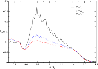
Figure 2: The interband transition for $(Q_{\parallel},Q_{\perp})=(\pi,\pi/2)$ found by exact diagonalization of a $J_{\parallel}=0.25J_{\perp}$ ladder system of $L=8$ rungs. The thermal broadening is much greater than $\eta=0.01$.

III Low Temperature Expansion

In what follows, we use the fact that for $J_{\parallel}\ll J_{\perp}$ states can still be labelled by their triplon number for $J_{\parallel}=0$, although it ceases to be a good quantum number for $J_{\parallel}\neq 0$. Subsequently, we will refer to the perturbative eigenstates as “$r$-particle states” $\left|{\gamma_{r}}\right\rangle$, where the terminology indicates that they reduce to $r$-triplon states when $J_{\parallel}$ is taken to zero. Here, $\gamma_{r}$ is a complete set of quantum numbers uniquely identifying the state under consideration. Using this notation, we rewrite Equation (7) as

$$\chi^{zz}(\omega,\mathbf{Q})\equiv\frac{1}{Z}\sum_{r,s=0}^{\infty}E_{r,s}+F_{r,s},$$

$$E_{r,s}=\frac{L}{2}\sum_{\gamma_{r},\gamma_{s}}\frac{e^{-\beta\epsilon_{\gamma_{r}}}}{\omega+i\eta+\epsilon_{\gamma_{r}}-\epsilon_{\gamma_{s}}}\delta_{Q_{\parallel}+p_{\gamma_{r}},p_{\gamma_{s}}}M_{\gamma_{r},\gamma_{s}},$$

$$F_{r,s}=-\frac{L}{2}\sum_{\gamma_{r},\gamma_{s}}\frac{e^{-\beta\epsilon_{\gamma_{s}}}}{\omega+i\eta+\epsilon_{\gamma_{r}}-\epsilon_{\gamma_{s}}}\delta_{Q_{\parallel}+p_{\gamma_{r}},p_{\gamma_{s}}}M_{\gamma_{r},\gamma_{s}}.$$ (8)

For sufficiently small $J_{\parallel}\ll J_{\perp}$, we may associate a formal temperature dependence with $E_{r,s}$ and $F_{r,s}$

$$E_{r,s}=\mathcal{O}\Bigl{(}e^{-\beta rJ_{\perp}}\Bigr{)},F_{r,s}=\mathcal{O}\Bigl{(}e^{-\beta sJ_{\perp}}\Bigr{)}.$$ (9)

Equation (I) becomes

$$M_{\gamma_{r},\gamma_{s}}=2\left|\left\langle{\gamma_{r}}\right|S^{z}_{0,0}\left|{\gamma_{s}}\right\rangle\right|^{2}\left(1+(-1)^{r-s}\cos(Q_{\perp})\right),$$ (10)

because due to the leg exchange symmetry

$$\left\langle{\gamma_{r}}\right|S^{z}_{0,0}(0)\left|{\gamma_{s}}\right\rangle=(-1)^{r-s}\left\langle{\gamma_{r}}\right|S^{z}_{1,0}(0)\left|{\gamma_{s}}\right\rangle.$$ (11)

The quantities $E_{r,s}$ and $F_{r,s}$ as well as the partition function $Z$ diverge in the thermodynamic limit. We therefore reorder the spectral sum in the spirit of a linked-cluster expansion following Ref. [EK09, ]. To do so, we express the partition function as

$$Z=\sum_{n=0}^{\infty}Z_{n},$$ (12)

where $Z_{n}$ is the contribution of $n$-particle states. It is furthermore convenient to combine quantities with the same formal temperature dependence as

$$G_{r,s}=E_{r,s}+F_{s,r}.$$ (13)

We then define the quantities

$$\mathcal{C}_{0}= \sum_{j=1}^{\infty}G_{0,j},$$

$$\mathcal{C}_{1}= G_{1,0}+\sum_{j=1}^{\infty}\Big{(}G_{1,j}-Z_{1}G_{0,j-1}\Big{)},$$

$$\mathcal{C}_{2}= G_{2,0}+\Big{(}G_{2,1}-Z_{1}G_{1,0}\Big{)}$$

$$+\sum_{m=2}^{\infty}\Big{(}G_{2,m}-Z_{1}G_{1,m-1}+(Z_{1}^{2}-Z_{2})G_{0,m-2}\Big{)},$$

$$\mathcal{C}_{3}= \dots$$ (14)

The $\mathcal{C}_{n}$ are the sums of all cluster functions with the same formal temperature dependence. Hence we obtain by construction that (as the triplon bandwidth is small compared to the triplon gap)

$$\mathcal{C}_{n}=\mathcal{O}(e^{-\beta nJ_{\perp}}).$$ (15)

We can then re-express the spectral sum in (5) as

$$\chi^{zz}(\omega,{\bf Q})=\frac{1}{Z}\sum_{r,s=0}^{\infty}\left(E_{r,s}+F_{r,s}\right)=\sum_{n=0}^{\infty}\mathcal{C}_{n}.$$ (16)

Now we postulate that $\mathcal{C}_{n}$ are finite in the thermodynamic limit and (16) constitutes a low-temperature expansion. This assumption is valid in the limit of non-interacting dimers $J_{\parallel}=0$. We furthermore verify it by explicit calculation for the leading contribution $\mathcal{C}_{1}$ for $J_{\parallel}\neq 0$. By virtue of the existence of a spectral gap $\Delta$ the contribution of $\mathcal{C}_{n}$ is seen to be proportional to $e^{-n\Delta/T}$, so that (16) constitutes a low-temperature expansion in the small parameter $e^{-\Delta/T}$, which can be viewed as the density of triplons in the state of thermal equilibrium.

III.1 Divergences

As we will see, the expansion (16) exhibits “infrared” divergences at

1. $\omega\to\pm\epsilon(Q_{\parallel})$. These occur in the “interband transition” terms $G_{j,j+1}$.

2. $\omega\to\pm 2J_{\parallel}\sin(Q_{\parallel}/2)$. These occur in the “intraband transition” terms $G_{j,j}$.

In order to deal with these divergences, we need to sum up an infinite number of terms in the low-temperature expansion. This can be done by following Refs. [EK08, ; JEK08, ].

III.1.1 “Interband” processes

The expansion (16) contains as the leading term the $T=0$ result, which diverges when the external frequency $\omega$ approaches the single-triplon dispersion $\epsilon(Q_{\parallel})$ like

$$\frac{1}{(\omega+i\eta)^{2}-\epsilon^{2}(Q_{\parallel})}.$$ (17)

This corresponds to the coherent propagation of a single triplon at $T=0$ and leads to a contribution proportional to $\delta(\omega^{2}-\epsilon^{2}(Q_{\parallel}))$ in the DSF. On the other hand, for any finite temperature we expect this delta-function to be broadened. This is a non-perturbative effect and cannot be captured in any finite order in the expansion (16). The fact that a broadening occurs emerges from the occurrence of “infrared” divergences in (16), i.e. singularities when the external frequency $\omega$ approaches the single-triplon dispersion $\epsilon(Q_{\parallel})$. For example, we show below that the first sub-leading contribution $\mathcal{C}_{1}$ exhibits a divergence

$$\left(\frac{1}{(\omega+i\eta)^{2}-\epsilon^{2}(Q_{\parallel})}\right)^{2}.$$ (18)

We expect the higher terms in the expansion to exhibit ever stronger divergences of this type, which need to be summed up in order to obtain a physically meaningful result. This can be achieved by employing a self-energy formalism EK08 ; JEK08 . To deal specifically with the divergence at $\omega^{2}=\epsilon^{2}(Q_{\parallel})$, we divide the expansion (16) for the susceptibility into a singular (for $\omega^{2}\to\epsilon^{2}(Q_{\parallel})$) and a regular piece as follows

$$\chi^{zz}(\omega,\mathbf{Q})=\chi^{zz}_{\mathrm{sing},1}(\omega,\mathbf{Q})+\chi^{zz}_{\mathrm{reg}}(\omega,\mathbf{Q}).$$ (19)

We then introduce a self-energy $\Sigma_{1}(\omega,\mathbf{Q})$ by expressing the singular contribution to the dynamical susceptibility in the form of

$$\chi^{zz}_{\mathrm{sing},1}(\omega,\mathbf{Q}) =\frac{G_{0,1}(\omega,\mathbf{Q})}{1-G_{0,1}(\omega,\mathbf{Q})\Sigma_{1}(\omega,\mathbf{Q})}$$

$$=G_{0,1}(\omega,\mathbf{Q})+G_{0,1}^{2}(\omega,\mathbf{Q})\Sigma_{1}(\omega,\mathbf{Q})+\cdots.$$ (20)

Here $G_{0,1}(\omega,\mathbf{Q})$ is the singular contribution to the leading term $\mathcal{C}_{0}$ in the expansion (16). Matching (III.1.1) to (16) then yields a low-temperature expansion of both $\chi_{\mathrm{reg}}(\omega,{\bf Q})$ and the self-energy

$$\Sigma_{1}(\omega,\mathbf{Q})=\sum_{j=1}^{\infty}\Sigma_{1}^{(j)}(\omega,\mathbf{Q}),$$ (21)

where the formal temperature dependence of the $n^{\mathrm{th}}$ contribution is

$$\Sigma_{1}^{(n)}(\omega,\mathbf{Q})=\mathcal{O}\Bigl{(}e^{-n\beta\Delta}\Bigr{)}.$$ (22)

III.1.2 “Intraband” Processes

In the intraband processes $G_{j,j}(\omega,\mathbf{Q})$ ($j=1,2$), we encounter singularities of the form

$$\Big{[}4J_{\parallel}^{2}\sin^{2}(Q_{\parallel}/2)-(\omega+i\eta)^{2}\Big{]}^{-j-1/2}.$$ (23)

We can deal with these singularities by employing a self-energy formalism in a way completely analogous to the way we proceeded for the interband processes. This results in a two-self-energy formalism for the dynamical susceptibility. We express $\chi^{zz}(\omega,\mathbf{Q})$ as a sum of three terms

$$\chi^{zz}(\omega,\mathbf{Q})=\chi^{zz}_{\mathrm{sing},1}(\omega,\mathbf{Q})+\chi^{zz}_{\mathrm{sing},2}(\omega,\mathbf{Q})+\chi^{zz}_{\mathrm{reg}}(\omega,\mathbf{Q}),$$ (24)

where $\chi^{zz}_{\mathrm{sing},1}(\omega,\mathbf{Q})$ and $\chi^{zz}_{\mathrm{sing},2}(\omega,\mathbf{Q})$ denote the contributions of all terms singular for $\omega^{2}\to\epsilon^{2}(Q_{\parallel})$ and $\omega^{2}\to 4J^{2}_{\parallel}\sin^{2}(Q_{\parallel}/2)$ respectively. The contribution $\chi^{zz}_{\mathrm{sing},2}(\omega,\mathbf{Q})$ defines a self-energy $\Sigma_{2}(\omega,\mathbf{Q})$ by

$$\chi^{zz}_{\mathrm{sing},2}(\omega,\mathbf{Q}) =\frac{G_{1,1}(\omega,\mathbf{Q})}{1-G_{1,1}(\omega,\mathbf{Q})\Sigma_{2}(\omega,\mathbf{Q})}$$

$$=G_{1,1}(\omega,\mathbf{Q})+G_{1,1}^{2}(\omega,\mathbf{Q})\Sigma_{2}(\omega,\mathbf{Q})+\dots$$

Matching the expansions (III.1.2) to the low-temperature expansion for $\chi^{zz}_{\mathrm{sing},2}(\omega,\mathbf{Q})$ generates a low-temperature expansion for the self-energy $\Sigma_{2}(\omega,\mathbf{Q})$.

IV Excited states in the limit of weak interdimer coupling

IV.1 Single triplon excited states

We start with the Hamiltonian (I). $\mathcal{H}_{0}$ is the dominant part of the Hamiltonian, which describes $L$ uncoupled dimers. The eigenstates of $\mathcal{H}_{0}$ are tensor products of singlet and triplet states at sites $n=0,\ldots,L-1$. The unique ground state of $\mathcal{H}_{0}$ is thus a series of singlet states on every site $n$. There are $3L$ degenerate first excited states that consist of $L-1$ singlets and one triplet. We treat $\mathcal{H}_{1}$ as a perturbation to $\mathcal{H}_{0}$ and construct a basis for one- and two-particle excited states.

We define an operator $d_{a}(m)$, which creates a triplet at site $a$ with $z$-component of spin $m$ when acting on the ground state $\left|{0}\right\rangle$. Single particle states with a definite value of momentum $p$ that carry spin-$1$ are constructed as

$$\left|{p,m}\right\rangle=\frac{1}{\sqrt{L}}\sum_{n=0}^{L-1}e^{ipn}d_{n}(m)\left|{0}\right\rangle.$$ (26)

With periodic boundary conditions $S_{L}\equiv S_{0}$, translational invariance makes momentum a good quantum number and the above states are orthogonal, which enables us to use non-degenerate perturbation theory to calculate the single particle energy shifts. To first order in $\alpha=J_{\parallel}/J_{\perp}$, the dispersion is given by

$$\epsilon_{p}=J_{\bot}+J_{\parallel}\cos(pa_{\parallel}),$$ (27)

where $a_{\parallel}$ is the separation between the dimers. Imposing periodic boundary conditions leads to the quantization of one-particle momenta

$$e^{ipL}=1.$$ (28)

IV.2 Two-triplon excited states

We now construct a basis of two particle states in which $\mathcal{H}_{1}$ is diagonal. To lowest order in $\alpha$, the two-particle states can be written as as

$$\left|{p_{1},p_{2},S,m}\right\rangle=\mathcal{N}_{S}(p_{1},p_{2})\sum_{a=1}^{L-1}\sum_{b=0}^{a-1}\psi^{S}_{a,b}(p_{1},p_{2})\phi^{S,m}_{a,b}\left|{0}\right\rangle,$$ (29)

where

$$\phi^{S,m}_{a,b}=\sum_{m_{1},m_{2}}\Phi^{S,m}_{m_{1},m_{2}}d_{a}(m_{1})d_{b}(m_{2}).$$ (30)

Here $\Phi^{S,m}$ are Clebsch-Gordan coefficients. The total spin takes values $S=0,1,2$ and the normalization $\mathcal{N}_{S}(p_{1},p_{2})$ depends on spin and linear momenta in general. The spatial part of the wavefunction is given by

$$\psi^{S}_{a,b}(p_{1},p_{2})=e^{i(p_{1}a+p_{2}b)}+A^{S}_{p_{1},p_{2}}e^{i(p_{1}b+p_{2}a)},$$ (31)

where the phase-shifts $A^{S}_{p_{1},p_{2}}$ encode triplon-triplon interactions. The boundary condition $\psi^{S}_{L-1,b}(p_{1},p_{2})\equiv(-1)^{S}\psi^{S}_{b,0}(p_{1},p_{2})$, where the sign is due to odd $S$ states being antisymmetric, leads to non-trivial quantization of two-particle momenta

$$(-1)^{S}A^{S}_{p_{1},p_{2}}=e^{ip_{1}L}=e^{-ip_{2}L}.$$ (32)

These equations require a numerical solution. Since for real momenta $A^{S}_{p_{1},p_{2}}$ is a pure phase, we introduce the notation

$$\delta^{S}_{p_{1},p_{2}}=-i\ln\left(A^{S}_{p_{1},p_{2}}\right).$$ (33)

The normalization of two-particle states is given by

$$\mathcal{N}_{S}(p_{1},p_{2})=\left[L\left(L-1\right)\right.\\ -\left.L\frac{\sin\left(\frac{1}{2}(p_{1}-p_{2})-\delta_{p_{1}p_{2}}^{S}\right)}{\sin\left(\frac{1}{2}(p_{1}-p_{2})\right)}\right]^{-1/2}.$$ (34)

The two-particle states have degeneracy $3^{2}\binom{L}{2}$. A basis of the two-particle subspace in which $\mathcal{H}_{1}$ is diagonal is constructed by requiring that

$$\mathcal{P}_{2}\mathcal{H}_{1}\left|{p_{1},p_{2},S,m}\right\rangle=(\epsilon_{p_{1}}+\epsilon_{p_{2}})\left|{p_{1},p_{2},S,m}\right\rangle.$$ (35)

Here $\mathcal{P}_{2}$ is the projection operator onto two-particle states. This leads to a condition on $A^{S}_{p_{1},p_{2}}$. When the triplets in the sum (27) are not on adjacent rungs, this condition is satisfied for any $A$. Considering the case of neighbouring triplets, we find

$$A^{0}_{p_{1},p_{2}} =-\frac{1+e^{-i(p_{1}+p_{2})}+2e^{-ip_{2}}}{1+e^{-i(p_{1}+p_{2})}+2e^{-ip_{1}}}$$

$$A^{1}_{p_{1},p_{2}} =-\frac{1+e^{-i(p_{1}+p_{2})}+e^{-ip_{2}}}{1+e^{-i(p_{1}+p_{2})}+e^{-ip_{1}}}$$

$$A^{2}_{p_{1},p_{2}} =-\frac{1+e^{-i(p_{1}+p_{2})}-e^{-ip_{2}}}{1+e^{-i(p_{1}+p_{2})}-e^{-ip_{1}}}.$$ (36)

The procedure for solving Equation (IV.2) is outlined in Appendix B. Without affecting the result in the thermodynamic limit, we simplify the calculation by considering $L$ to be even.

V Matrix elements

Table 1: Non-zero matrix elements of $S^{z}_{j,0}$ to order $\alpha$. For the definitions see (V.2), (V.3) and (A).

$\left\langle{0}\right|$$S^{z}_{j,0}$	$\left|{p,0}\right\rangle$	$(-1)^{j+1}\frac{1}{2\sqrt{L}}\left(1-\frac{\alpha}{2}\cos(p)\right)$
$\left\langle{p^{\prime},\pm 1}\right|$$S^{z}_{j,0}$	$\left|{p,\pm 1}\right\rangle$	$\pm\frac{1}{2L}$
$\left\langle{p_{1},p_{2},0,0}\right|$$S^{z}_{j,0}$	$\left|{p,0}\right\rangle$	$(-1)^{j+1}\sqrt{\frac{1}{12L^{3}}}\left(U_{0}(p,p_{1},p_{2})-\frac{\alpha}{2}V_{0}(p,p_{1},p_{2})\right)$
$\left\langle{p_{1},p_{2},1,\pm 1}\right|$$S^{z}_{j,0}$	$\left|{p,\pm 1}\right\rangle$	$\pm(-1)^{j}\sqrt{\frac{1}{8L^{3}}}\left(U_{1}(p,p_{1},p_{2})-\frac{\alpha}{2}V_{1}(p,p_{1},p_{2})\right)$
$\left\langle{p_{1},p_{2},2,0}\right|$$S^{z}_{j,0}$	$\left|{p,0}\right\rangle$	$(-1)^{j}\sqrt{\frac{1}{6L^{3}}}\left(U_{2}(p,p_{1},p_{2})-\frac{\alpha}{2}V_{2}(p,p_{1},p_{2})\right)$
$\left\langle{p_{1},p_{2},2,\pm 1}\right|$$S^{z}_{j,0}$	$\left|{p,\pm 1}\right\rangle$	$(-1)^{j}\sqrt{\frac{1}{8L^{3}}}\left(U_{2}(p,p_{1},p_{2})-\frac{\alpha}{2}V_{2}(p,p_{1},p_{2})\right)$
$\left\langle{p^{\prime}_{1},p^{\prime}_{2},1,\pm 1}\right|$$S^{z}_{j,0}$	$\left|{p_{1},p_{2},1,\pm 1}\right\rangle$	$\mp\frac{1}{4L^{2}}W_{1,1}(p^{\prime}_{1},p^{\prime}_{2},p_{1},p_{2})$
$\left\langle{p^{\prime}_{1},p^{\prime}_{2},2,\pm 2}\right|$$S^{z}_{j,0}$	$\left|{p_{1},p_{2},2,\pm 2}\right\rangle$	$\mp\frac{1}{2L^{2}}W_{2,2}(p^{\prime}_{1},p^{\prime}_{2},p_{1},p_{2})$
$\left\langle{p^{\prime}_{1},p^{\prime}_{2},2,\pm 1}\right|$$S^{z}_{j,0}$	$\left|{p_{1},p_{2},2,\pm 1}\right\rangle$	$\pm\frac{1}{4L^{2}}W_{2,2}(p^{\prime}_{1},p^{\prime}_{2},p_{1},p_{2})$
$\left\langle{p^{\prime}_{1},p^{\prime}_{2},2,\pm 1}\right|$$S^{z}_{j,0}$	$\left|{p_{1},p_{2},1,\pm 1}\right\rangle$	$\pm\frac{1}{4L^{2}}W_{2,1}(p^{\prime}_{1},p^{\prime}_{2},p_{1},p_{2})$
$\left\langle{p^{\prime}_{1},p^{\prime}_{2},2,0}\right|$$S^{z}_{j,0}$	$\left|{p_{1},p_{2},1,0}\right\rangle$	$\frac{1}{2\sqrt{3}L^{2}}W_{2,1}(p^{\prime}_{1},p^{\prime}_{2},p_{1},p_{2})$
$\left\langle{p^{\prime}_{1},p^{\prime}_{2},1,0}\right|$$S^{z}_{j,0}$	$\left|{p_{1},p_{2},0,0}\right\rangle$	$\frac{1}{2L^{2}}\sqrt{\frac{2}{3}}W_{1,0}(p^{\prime}_{1},p^{\prime}_{2},p_{1},p_{2})$

V.1 Selection rules

At low temperatures $T\ll J_{\perp}$, the leading terms in the expansion (16) involve states with at most two triplons (in the aforementioned sense that the corresponding states reduce to states with at most two triplets in the $J_{\parallel}=0$ limit). In the following we compute the matrix elements which link $0,1$ and $2$-particle states.

The operator $S^{z}_{j,l}$ acts on a single site, thus changing the triplon number by $\Delta n=0$ or $1$. To first order in $\alpha$, $\mathcal{H}_{1}$ mixes states with those differing in triplon number by $\Delta n=\pm 2$. As however we will only consider the modulus squared of the matrix elements, this correction is only relevant in the case that the matrix element is non-zero to leading order. The rule remains valid. $S^{z}_{j,l}$ conserves the total $S^{z}$ which we have used to label states, so $\Delta S^{z}=0$. The total spin $S$ has to obey the triangle rule. The operator under consideration is a vector, thus $|\Delta S|\leq 1$ and a transition where $S=0$ in both initial and final state is forbidden. As the operator is acting on a single site, when $\Delta S=0$ the $S^{z}=0$ states have a zero matrix element.

V.2 Interband matrix elements

The matrix elements will be expressed in terms of $U_{S}(p,p_{1},p_{2})$. There are several cases to consider for each of the types of solution listed in Appendix B, and their respective contributions are shown in Appendix C.1. The form for a real solution is

$$U_{S}(p,p_{1},p_{2})\equiv L\mathcal{N}_{S}(p_{1},p_{2})e^{-\frac{i}{2}\delta^{S}_{p_{1},p_{2}}}e^{i\frac{\pi}{2}S}$$

$$\times\left[\frac{\sin\left(\frac{1}{2}(p-p_{1}+\delta^{S}_{p_{1},p_{2}}-\pi S)\right)}{\sin\left(\frac{1}{2}(p-p_{1})\right)}\right.$$

$$+\left.\frac{\sin\left(\frac{1}{2}(p-p_{2}-\delta^{S}_{p_{1},p_{2}}-\pi S)\right)}{\sin\left(\frac{1}{2}(p-p_{2})\right)}\right].$$ (37)

We also calculate the perturbative correction to the matrix elements to order $\mathcal{O}\left(\alpha\right)$ in Appendix C.3. The relevant matrix elements are given in Table 1.

V.3 Intraband matrix elements

In the two triplon sector, transitions are possible between most combinations of states listed in Appendix B. The full list is shown in Appendix C.2. The result for transitions between real states is

$$W_{S^{\prime},S}(p^{\prime}_{1},p^{\prime}_{2},p_{1},p_{2})=$$

$$\qquad L^{2}\mathcal{N}_{S}(p_{1},p_{2})\mathcal{N}_{S^{\prime}}(p^{\prime}_{1},p^{\prime}_{2})e^{\frac{i}{2}(\delta^{S}_{p_{1},p_{2}}-\delta^{S^{\prime}}_{p^{\prime}_{1},p^{\prime}_{2}}+(S^{\prime}-S)\pi)}$$

$$\times\biggl{[}\frac{\sin(\frac{1}{2}(p_{1}-p^{\prime}_{1}-\delta^{S}_{p_{1},p_{2}}+\delta^{S^{\prime}}_{p^{\prime}_{1},p^{\prime}_{2}}-(S^{\prime}-S)\pi))}{\sin(\frac{1}{2}(p_{1}-p^{\prime}_{1}))}$$

$$+\frac{\sin(\frac{1}{2}(p_{1}-p^{\prime}_{2}-\delta^{S}_{p_{1},p_{2}}-\delta^{S^{\prime}}_{p^{\prime}_{1},p^{\prime}_{2}}-(S^{\prime}-S)\pi))}{\sin(\frac{1}{2}(p_{1}-p^{\prime}_{2}))}$$

$$+\frac{\sin(\frac{1}{2}(p_{2}-p^{\prime}_{1}+\delta^{S}_{p_{1},p_{2}}+\delta^{S^{\prime}}_{p^{\prime}_{1},p^{\prime}_{2}}-(S^{\prime}-S)\pi))}{\sin(\frac{1}{2}(p_{2}-p^{\prime}_{1}))}$$

$$+\frac{\sin(\frac{1}{2}(p_{2}-p^{\prime}_{2}+\delta^{S}_{p_{1},p_{2}}-\delta^{S^{\prime}}_{p^{\prime}_{1},p^{\prime}_{2}}-(S^{\prime}-S)\pi))}{\sin(\frac{1}{2}(p_{2}-p^{\prime}_{2}))}\biggr{]}.$$ (38)

In the cases that either of the momenta in the first state equals either of those in the second, the corresponding fraction needs to be replaced by

$$-(L-1)e^{\frac{i}{2}(\pm\delta^{S}_{p_{1},p_{2}}\mp\delta^{S^{\prime}}_{p^{\prime}_{1},p^{\prime}_{2}}-(S^{\prime}-S)\pi)}.$$

VI Spectral representation and resummation

The leading contributions to the low-temperature expansion for the dynamical susceptibility are given by $G_{0,1}=E_{0,1}+F_{1,0}$. Using the matrix elements from Table 1, we find that to order $\alpha$ we have

$$G_{0,1}= \frac{(1-\cos{Q_{\perp}})}{4}(1-\alpha\cos{Q_{\parallel}})$$

$$\times\left(\frac{1}{\omega+i\eta-\epsilon_{Q_{\parallel}}}-\frac{1}{\omega+i\eta+\epsilon_{Q_{\parallel}}}\right).$$ (39)

These give rise to a delta function peak located at the one-triplon excitation energy. The intraband term $G_{1,1}$ is given by

$$G_{1,1}=\frac{(1+\cos{Q_{\perp}})}{2L}\sum_{p}\frac{e^{-\beta\epsilon_{p}}-e^{-\beta\epsilon_{Q_{\parallel}+p}}}{\omega+i\eta+\epsilon_{p}-\epsilon_{Q_{\parallel}+p}}.$$ (40)

Similarly, we find the interband terms

$$G_{1,2}= \frac{(1-\cos{Q_{\perp}})}{4L^{2}}\sum_{p_{1}>p_{2}}(e^{-\beta\epsilon_{Q_{\parallel}+p_{1}+p_{2}}}$$

$$\times\left(\frac{1}{\omega+i\eta+\epsilon_{Q_{\parallel}+p_{1}+p_{2}}-\epsilon_{p_{1}}-\epsilon_{p_{2}}}\right.$$

$$-\left.\frac{1}{\omega+i\eta+\epsilon_{p_{1}}+\epsilon_{p_{2}}-\epsilon_{Q_{\parallel}+p_{1}+p_{2}}}\right)$$

$$\times\sum_{S}\frac{2S+1}{3}(|U_{S}^{2}-\alpha U_{S}V_{S}|).$$ (41)

The sum over $p_{1},p_{2}$ is taken over all momenta that satisfy the boundary conditions (32), and these momenta depend on $S$. The leading term in $G_{1,2}$ scales with $L$, but cancels against the “disconnected” contribution $Z_{1}G_{0,1}$. The low-temperature expansion of the dynamical susceptibility now takes the form

$$\chi^{zz}(\omega,\mathbf{Q})\approx\mathcal{C}_{0}+\mathcal{C}_{1}+\mathcal{C}_{2},$$ (42)

where

$$\mathcal{C}_{0}(\omega,{\bf Q}) \approx G_{0,1},$$

$$\mathcal{C}_{1}(\omega,{\bf Q}) \approx G_{1,0}+G_{1,1}+\Bigl{(}G_{1,2}-Z_{1}G_{0,1}\Bigr{)},$$

$$\mathcal{C}_{2}(\omega,{\bf Q}) \approx G_{2,2}-Z_{1}G_{1,1}.$$ (43)

Here $Z_{1}=3\sum_{p}e^{-\beta\epsilon_{p}}$ is the single particle contribution to the partition function. We note that in $\mathcal{C}_{2}$ we only have taken into account the intraband processes. We observe the following divergences in $\mathcal{C}_{n}$:

$$\mathcal{C}_{n}(\omega,Q_{\parallel})\propto\begin{cases}\left(\frac{1}{(\omega+i\eta)^{2}-\epsilon^{2}(Q_{\parallel})}\right)^{1+n}&\omega^{2}\approx\epsilon^{2}_{Q_{\parallel}},\cr\left(\frac{1}{\varepsilon^{2}(Q_{\parallel})-(\omega+i\eta)^{2}}\right)^{n-1/2}&\omega^{2}\approx\varepsilon^{2}_{Q_{\parallel}},\cr\end{cases}$$ (44)

where we have defined

$$\varepsilon(k)=2J_{\parallel}\sin(Q_{\parallel}/2).$$ (45)

The first (second) kind of singularity is seen to be present in $\mathcal{C}_{n}$ for $n=0,1$ ($n=1,2$). We expect (44) to hold for $n\geq 2$ as well. Following the procedure set out in Section III.1, we define

$$\chi^{zz}_{\mathrm{sing},2} \approx G_{1,1}+(G_{2,2}-Z_{1}G_{1,1}),$$

$$\chi^{zz}_{\mathrm{sing},1} \approx G_{0,1}+G_{1,0}+(G_{1,2}-Z_{1}G_{0,1}).$$ (46)

The leading orders in the low-temperature expansions of the self-energies then take the form

$$\Sigma_{1}(\omega,\mathbf{Q}) =G_{0,1}^{-2}(\omega,\mathbf{Q})\left[G_{1,2}(\omega,\mathbf{Q})-Z_{1}G_{0,1}(\omega,\mathbf{Q})\right],$$

$$\Sigma_{2}(\omega,\mathbf{Q}) =G_{1,1}^{-2}(\omega,\mathbf{Q})\left[G_{2,2}(\omega,\mathbf{Q})-Z_{1}G_{1,1}(\omega,\mathbf{Q})\right].$$

Our approximate result for the DSF is then

$$S^{zz}(\omega,\mathbf{Q})= -\lim_{\eta\rightarrow 0}\frac{1}{\pi}\frac{1}{1-e^{-\beta\omega}}$$

$$\times\Im\Biggl{[}\frac{G_{1,1}(\omega,\mathbf{Q})}{1-G_{1,1}(\omega,\mathbf{Q})\Sigma_{2}(\omega,\mathbf{Q})}$$

$$\qquad+\frac{G_{0,1}(\omega,\mathbf{Q})}{1-G_{0,1}(\omega,\mathbf{Q})\Sigma_{1}(\omega,\mathbf{Q})}\Biggr{]}.$$ (48)

VII Results and discussion

In order to present explicit results, we choose $\alpha=0.1$ and perform numerical calculations on a system of $L=1000$ dimers. Doubling the number did not change the results significantly. The limit $\eta\rightarrow 0$ is approximated by choosing a value larger than the spacing of the momentum values due to finite size, which is of order $\mathcal{O}(\frac{4\pi}{L}J_{\parallel})$, but small compared to the thermal broadening $J_{\parallel}e^{-\beta J_{\perp}}$, so that the shape of the response is not changed significantly. One problem we encounter is that to the order in $J_{\parallel}/J_{\perp}$ we are working in, the bound state contributions to $\mathcal{C}_{1}$ give rise to sharp peaks for kinematic reasons. These features will be suppressed once higher orders in perturbation theory are taken into account, even if we do not sum higher order terms in the low-temperature expansion (which would lead to a further broadening). Given that the sharp bound state peaks are an artifact of the order in perturbation theory considered, we choose to suppress them in the various plots by specifying a sufficiently large broadening $\eta=0.01$. This also facilitates comparison to the ED results. The choice of $Q_{\perp}$ affects the mixing between the intraband ($\propto\cos^{2}\frac{1}{2}Q_{\perp}$) and interband ($\propto\sin^{2}\frac{1}{2}Q_{\perp}$) responses. Hence plots are given for $Q_{\perp}=\pi/2$, where both types of transition are allowed with equal weight.

VII.1 Broadening of the triplon line

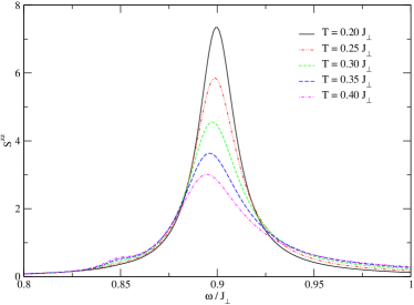
Figure 3: The interband transition for $(Q_{\parallel},Q_{\perp})=(\pi,\pi/2)$ and $L=1000$ sites. The asymmetry grows as $T$ increases.

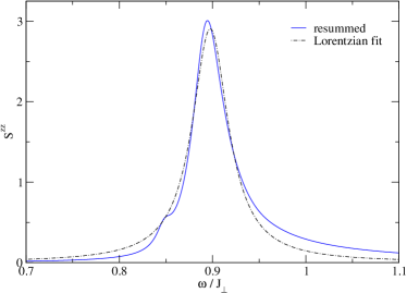
Figure 4: The resummed interband transition lineshape for $T=0.4J_{\perp}$, $Q_{\perp}=\pi/2$, $Q_{\parallel}=\pi$, $\eta=0.01$ and $L=1000$ together with a Lorentzian best fit demonstrating the asymmetric lineshape.

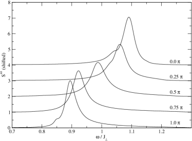
Figure 5: Dependence of the interband transition at $T=0.5J_{\perp}$ on $Q_{\parallel}$. $Q_{\perp}$ is fixed at $\pi/2$ and $L=1000$. The graphs are offset by $n$ for $Q_{\parallel}=n\pi/4$.

We first consider the temperature evolution of the triplon line. At $T=0$ the DSF features a delta function line following the triplon dispersion. In Fig. 3, we plot $S^{zz}(\omega,{\bf Q})$ as a function of frequency for wave vector ${\bf Q}=(\pi,\pi/2)$ and temperatures in the range $0.2J_{\perp}\leq T\leq 0.4J_{\perp}$. We see that the line broadens asymmetrically in energy as the temperature increases. On the other hand, at sufficiently low temperatures we expect the lineshape to be well approximated by a Lorentzian damle . In Fig. 4, we show a comparison of the actual result to a Lorentzian fit

$$S_{\mathrm{Lor}}(\omega,\mathbf{Q})=A(\mathbf{Q})\frac{1/\tau_{\phi}}{(\omega-\epsilon(Q_{\parallel}))^{2}+1/\tau_{\phi}^{2}}.$$ (49)

Fig. 5 shows the dependence of the asymmetry on $Q_{\parallel}$. The falloff is slower towards the centre of the dispersion. In order to establish the temperature range in which our low-temperature expansion provides accurate results, we compare (48) to numerical results obtained by a direct diagonalization of the Hamiltonian for short chains. To obtain a continuous curve for the DSF, we convolve the numerical results with a Lorentzian of width $\eta=0.02$. Fig. 6 shows such a comparison for $T=0.4J_{\perp}$, $Q_{\perp}=\pi/2$, $Q_{\parallel}=\pi$ and $L=1000$. We see that there is good agreement between the two methods.

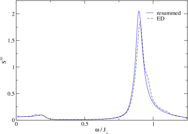
Figure 6: A comparison of the resummed spectral function for $T=0.4J_{\perp}$, $Q_{\perp}=\pi/2$, $Q_{\parallel}=\pi$, $\eta=0.02$ and $L=1000$ to the ED result for a $L=8$ system.

VII.2 Finite temperature resonance at low frequencies

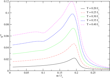
Figure 7: The intraband transition at a series of temperatures. $Q_{\perp}=\pi/2$, $Q_{\parallel}=\pi$, $\eta=0.01$ and $L=1000$.

As in the state of thermal equilibrium there is a finite density of triplons, incident neutrons can scatter off them with energy transfers small compared to the gap. Accordingly at finite temperatures there is a spin response at energies $\omega\sim 0$. To leading contribution to this “intraband response” is

$$-\frac{1}{\pi}\frac{1}{1-e^{-\beta\omega}}\Im G_{1,1}=\frac{1+\cos(Q_{\perp})}{2\pi}\frac{e^{-\beta(J-\omega/2)}}{\sqrt{\varepsilon^{2}(Q_{\parallel})-\omega^{2}}}$$

$$\times\cosh\left(\frac{\beta\cot(Q_{\parallel}/2)}{2}\sqrt{\varepsilon^{2}(Q_{\parallel})-\omega^{2}}\right)\theta\left(\varepsilon^{2}(Q_{\parallel})-\omega^{2}\right),$$ (50)

where $\varepsilon(Q_{\parallel})$ is given by (45). This contribution contains square root singularities for $\omega\to\pm\varepsilon(Q_{\parallel})$, which get smoothened once we resum terms following Section III.1.2. In Fig. 7 we plot the DSF at low frequencies for several temperatures in the range $0.2J_{\perp}\leq T\leq 0.4J_{\perp}$. We see that the integrated intensity increases with temperature, while a strong peak at $\omega\approx\varepsilon(Q_{\parallel})$ remains. This is very similar to what happens in the spin-$\frac{1}{2}$ Heisenberg-Ising chain JGE , where this feature was first predicted by Villain villain .

VII.3 Summary

In this work we have determined the low temperature dynamical structure factor of the two-leg spin-$\frac{1}{2}$ Heisenberg ladder in the limit where the leg coupling is weak compared to the rung exchange. We have shown that the sharp delta-function line following the triplon dispersion at $T=0$ gets broadened in an asymmetric way at $T>0$. The dominant processes at low $T$ involve scattering from one-triplon to two-triplon states in the presence of a “thermal background”, as described in Section III. We have also determined the temperature activated contribution to the DSF at low frequencies. Here the dominant processes at low $T$ involve scattering between different two-triplon states in the presence of a “thermal background”. Our analysis is based on the method developed in Ref. [JEK08, ] for the case of the alternating spin-$\frac{1}{2}$ Heisenberg chain. We have gone beyond Ref. [JEK08, ] in two important aspects. Firstly, we have taken into account all perturbative corrections to the various matrix elements to order $\mathcal{O}\left(J_{\parallel}/J_{\perp}\right)$. This establishes that higher order perturbation theory in $J_{\parallel}/J_{\perp}$ can be combined with the low-temperature expansion of Ref. [JEK08, ]. Secondly, we have included the order $\mathcal{O}\left(e^{-2\beta J_{\perp}}\right)$ correction $G_{2,2}-Z_{1}G_{1,1}$ to the intraband contribution. This allows us to describe the low-frequency temperature induced “resonance” in a significantly larger temperature window and demonstrates the difficulties encountered when dealing with higher orders in the low-temperature expansion. It would be interesting to compare our results to experiments on ladder materials. Perhaps the best candidate is $\rm(C_{5}H_{12}N)_{2}CuBr_{4}$, which is a highly one-dimensional two-leg ladder material with $\alpha\approx 0.256$ RueggA ; RueggB ; RueggC . Experimental studies of the temperature evolution of the DSF for this material are under way Ruegg2 .

Appendix A Linked-cluster expansion for $J_{\parallel}=0$

For $J_{\parallel}=0$ we are dealing with an ensemble of uncoupled dimers. The dynamical susceptibility can then be calcuated by elementary means in the Matsubara formalism. After analytic continuation we obtain

$$\chi^{zz}(\omega>0,\mathbf{Q})=\frac{J_{\perp}}{2}\frac{1-e^{-\beta J_{\perp}}}{1+3e^{-\beta J_{\perp}}}\frac{1-\cos(Q_{\perp})}{(\omega+i0)^{2}-J_{\perp}^{2}}.$$ (51)

The temperature dependent factor can be expanded at low temperatures

$$\frac{1-e^{-\beta J_{\perp}}}{1+3e^{-\beta J_{\perp}}}=1-4e^{-\beta J_{\perp}}+12e^{-2\beta J_{\perp}}+\ldots.$$ (52)

We have calculated the first few terms of the low-temperature expansion (16) by working in a product basis of dimer triplet and singlet states. The leading contribution is

$$\mathcal{C}_{0}=G_{0,1}=\frac{J_{\perp}}{2}\frac{1-\cos(Q_{\perp})}{(\omega+i0)^{2}-J_{\perp}^{2}},$$ (53)

which correctly reproduces the $T=0$ limit of (51). The next term is

$$\mathcal{C}_{1}=G_{1,0}+(G_{1,2}-Z_{1}G_{0,1}).$$ (54)

We find by explicit calculation that

$$G_{1,2}-Z_{1}G_{0,1}=-3e^{-\beta J_{\perp}}G_{0,1}.$$ (55)

This results in

$$\mathcal{C}_{1}=-4e^{-\beta J_{\perp}}G_{0,1},$$ (56)

which correctly reproduces the first subleading term in (51). The next term is

$$\mathcal{C}_{2}= (G_{2,1}-Z_{1}G_{1,0})$$

$$+(G_{2,3}-Z_{1}G_{1,2}+(Z_{1}^{2}-Z_{2})G_{0,1}).$$ (57)

We find that

$$G_{2,1}-Z_{1}G_{1,0} =-3e^{-\beta J_{\perp}}G_{0,1},$$

$$G_{2,3}-Z_{1}G_{1,2}+(Z_{1}^{2}-Z_{2})G_{0,1} =9e^{-2\beta J_{\perp}}G_{0,1},$$ (58)

which gives

$$\mathcal{C}_{2}=12e^{-\beta J_{\perp}}G_{0,1}.$$ (59)

This correctly reproduces the second subleading term in (51). We note that in the limit $J_{\parallel}=0$ the low-temperature expansion (16) is well defined and does not suffer from the kind of “infrared” divergences present for $J_{\parallel}\neq 0$. This is as expected since the spectral function of the full result (51) features a sharp delta-function line even at $T>0$.

Appendix B Solutions of the BAE

B.1 Real solutions

To find the two-triplon momenta allowed by the quantization condition (32), we follow the approach outlined by James et al. JEK08 . We choose a suitable branch cut such that the solutions are enumerated by

$$Lp_{1,2}=\mp i\ln(-A^{S}_{p_{1},p_{2}})+2\pi\left[I_{1,2}+\frac{1+(-1)^{S}}{4}\right],$$ (60)

where $I_{1,2}$ are integers used to parametrize the equation. This gives $L(L-1)/2$ possible solutions. To satisfy $p_{1}>p_{2}$ we need $I_{1}\geq I_{2}$. In the case of $I_{1}\neq I_{2}$ this is easily solved numerically, although care must be taken not to double-count solutions.

One must be careful with those solutions where the phase shift is zero. The momenta are then equal to the single triplon momenta and so the matrix elements can be of order $\mathcal{O}(L)$. These solutions occur only for $S=0$ or $2$. For these states the normalization is

$$\mathcal{N}_{S}=\left[L(L-2)\right]^{-\frac{1}{2}}.$$ (61)

The procedure above does not identify all real solutions in the $S=0$ sector. The remaining roots are found following Ref. [essxxx, ]. For large systems Equation (60) has solutions where $I_{1}=I_{2}$. Whereas the trivial solution $p_{1}=p_{2}$ is forbidden by the Pauli principle, another solution appears very close to the trivial one. Due to the proximity of the two zeros, the numerical solution of the equation is difficult. One method is to rewrite the BAE as a single equation in $x=p_{1}-p_{2}$ and to then divide by $x$ to eliminate the trivial zero, after which the root finder converges reliably on the desired solution.

B.2 Bound states

There also exist complex solutions $p_{1,2}=x\pm iy$, where the amplitude decays exponentially as a function of the separation of triplons, corresponding to bound states. For these the S-matrix elements are real, and equation (32) becomes

$$e^{ixL}e^{-yL}+(-1)^{S}\frac{2\cos(x)+(2-\frac{S}{2}(S+1))e^{-y}}{2\cos(x)+(2-\frac{S}{2}(S+1))e^{y}}=0.$$ (62)

For each $x=n\pi/L$ there may exist a zero, and the number of solutions scales as $L$. The matrix elements for these roots require special treatment and are given as previously in terms of

$$\mathcal{N}_{S}(p_{1},p_{1}^{*}) =\left[L(L-1)A^{S}_{p_{1},p_{1}^{*}}(-1)^{S}\right.$$

$$+\left.L\frac{e^{-y}-e^{y}(A^{S}_{p_{1},p_{1}^{*}})^{2}}{2\sinh(y)}\right]^{-\frac{1}{2}}.$$ (63)

B.3 Singular solutions (type I)

At this point we still miss $4$ solutions, which occur at singularities of the quantization conditions. Such a solution was described for the spin-$\frac{1}{2}$ XXX model in Ref. [essxxx, ]. For each $S$ sector there is a solution at $p_{1,2}=\pi/2\pm i\infty$, corresponding to a vanishing S-matrix eigenvalue. By introducing a twist angle $\phi$ the quantization conditions become

$$A^{S}_{p_{1},p_{2}}e^{i\phi/2} =(-1)^{S}e^{iLp_{1}},$$

$$e^{i\phi} =e^{iL(p_{1}+p_{2})}.$$ (64)

This renders the momenta finite, but they cease to be complex conjugate to one another. Normalizing the wave function and then taking the limit $\phi\rightarrow 0$ we obtain

$$\psi^{S}_{a,b}=(-1)^{b}(\delta_{a-1,b}-(-1)^{S}\delta_{a,L-1}\delta_{b,0}).$$ (65)

It can be verfied by direct calculation that this gives an eigenstate of the Hamiltonian. The normalization of the state is

$$\mathcal{N}_{S}=L^{-\frac{1}{2}}.$$ (66)

B.4 Singular solutions (type II)

Finally, there is another singular solution in the $S=0$ sector with $p_{1}=p_{2}=\pi$. This solution gives rise to an eigenstate despite the fact that the two momenta are the same because the phase shift is ill-defined. Again the limiting wave function can be calculated by introducing a twist angle, normalizing the state and then taking the twist angle to zero. The result for the wavefunction and its normalization is

$$\psi^{0}_{a,b} =(-1)^{a+b}$$ (67)

$$\mathcal{N}_{0} =\left(\frac{L(L-1)}{2}\right)^{-\frac{1}{2}}$$ (68)

Appendix C Matrix elements

C.1 Interband matrix elements

The interband matrix elements for the different types of solution are as follows:

1. Real solutions with zero phase shift:

   $$U_{S}(p,p_{1},p_{2})=-L\mathcal{N}_{S}\left(L\left(\delta_{p_{1},p}+\delta_{p_{2},p}\right)-2\right).$$ (69)

2. Bound states:

   $$U_{S}(p,p_{1},p_{1}^{*})= L\mathcal{N}_{S}(p_{1},p_{1}^{*})e^{i\frac{\pi S}{2}}\frac{1}{\cosh(y)-\cos(x-p)}$$

   $$\times\Biggl{[}(1+A^{S}_{p_{1},p_{1}^{*}})\cos(x-p-\frac{\pi S}{2})$$

   $$\qquad-(e^{-y}+A^{S}_{p_{1},p_{1}^{*}}e^{y})\cos(\frac{\pi S}{2})\Biggr{]}.$$ (70)

3. Singular solutions (type I):

   $$U_{S}(p)=2iL\mathcal{N}_{S}\sin(p).$$ (71)

4. Singular solution (type II):

   $$U_{0}(p)=L\mathcal{N}_{0}.$$ (72)

C.2 Intraband matrix elements

The intraband matrix elements are as follows for transitions between different types of states in the two triplon sector:

1. Real $\rightarrow$ Bound:

   $$W_{S^{\prime},S}(p^{\prime}_{1},{p^{\prime}}^{*}_{1},p_{1},p_{2})\equiv$$

   $$\qquad L^{2}\mathcal{N}_{S}(p_{1},p_{2})\mathcal{N}_{S^{\prime}}(p^{\prime}_{1},{p^{\prime}}^{*}_{1})e^{\frac{i}{2}(S^{\prime}-S)\pi}e^{\frac{i}{2}\delta^{S}_{p_{1},p_{2}}}$$

   $$\times\biggl{[}\frac{(A^{S^{\prime}}_{p^{\prime}_{1},{p^{\prime}}^{*}_{1}}e^{y}+e^{-y})\cos((S-S^{\prime})\frac{\pi}{2}+\frac{1}{2}\delta^{S}_{p_{1},p_{2}})}{\cos(p_{1}-x)-\cosh(y)}$$

   $$-\frac{(A^{S^{\prime}}_{p^{\prime}_{1},{p^{\prime}}^{*}_{1}}+1)\cos(x-p_{1}-(S-S^{\prime})\frac{\pi}{2}-\frac{1}{2}\delta^{S}_{p_{1},p_{2}})}{\cos(p_{1}-x)-\cosh(y)}$$

   $$+\frac{(A^{S^{\prime}}_{p^{\prime}_{1},{p^{\prime}}^{*}_{1}}e^{y}+e^{-y})\cos((S-S^{\prime})\frac{\pi}{2}-\frac{1}{2}\delta^{S}_{p_{1},p_{2}})}{\cos(p_{2}-x)-\cosh(y)}$$

   $$-\frac{(A^{S^{\prime}}_{p^{\prime}_{1},{p^{\prime}}^{*}_{1}}+1)\cos(x-p_{2}-(S-S^{\prime})\frac{\pi}{2}+\frac{1}{2}\delta^{S}_{p_{1},p_{2}})}{\cos(p_{2}-x)-\cosh(y)}\biggr{]}.$$ (73)

2. Real $\rightarrow$ Singular (type I):

   $$W_{S^{\prime},S}(\frac{\pi}{2},\frac{\pi}{2},p_{1},p_{2})\equiv$$

   $$\qquad L^{2}\mathcal{N}_{S}(p_{1},p_{2})\mathcal{N}_{S^{\prime}}e^{\frac{i}{2}(\delta^{S}_{p_{1},p_{2}}+(S^{\prime}-S)\pi)}$$

   $$\times 2\biggl{[}\cos\left(p_{1}-\frac{\delta^{S}_{p_{1},p_{2}}}{2}-(S^{\prime}-S)\frac{\pi}{2}\right)$$

   $$\qquad+\cos\left(p_{2}+\frac{\delta^{S}_{p_{1},p_{2}}}{2}-(S^{\prime}-S)\frac{\pi}{2}\right)\biggr{]}.$$ (74)

3. Real $\rightarrow$ Singular (type II):

   $$W_{0,1}(\pi,\pi,p_{1},p_{2})\equiv$$

   $$\qquad-iL^{2}\mathcal{N}_{1}(p_{1},p_{2})\mathcal{N}_{0}e^{\frac{i}{2}\delta^{S}_{p_{1},p_{2}}}$$

   $$\times\cos\frac{\delta^{S}_{p_{1},p_{2}}}{2}\left[\tan\frac{p_{1}}{2}+\tan\frac{p_{2}}{2}\right].$$ (75)

4. Bound $\rightarrow$ Bound:

   $$W_{S^{\prime},S}(p^{\prime}_{1},{p^{\prime}}^{*}_{1},p_{1},p^{*}_{1})\equiv$$

   $$\qquad L^{2}\mathcal{N}_{S}(p_{1},p^{*}_{1})\mathcal{N}_{S^{\prime}}(p^{\prime}_{1},{p^{\prime}}^{*}_{1})e^{i(x-x^{\prime})}$$

   $$\times\biggl{[}e^{-y-y^{\prime}}\frac{1-(-1)^{S+S^{\prime}}A^{S}_{p_{1},{p}^{*}_{1}}A^{S^{\prime}}_{p^{\prime}_{1},{p^{\prime}}^{*}_{1}}e^{-i(x-x^{\prime})+y+y^{\prime}}}{1-e^{i(x-x^{\prime})-y-y^{\prime}}}$$

   $$+e^{-y+y^{\prime}}\frac{A^{S^{\prime}}_{p^{\prime}_{1},{p^{\prime}}^{*}_{1}}-(-1)^{S+S^{\prime}}A^{S}_{p_{1},{p}^{*}_{1}}e^{-i(x-x^{\prime})+y-y^{\prime}}}{1-e^{i(x-x^{\prime})-y+y^{\prime}}}$$

   $$+e^{y-y^{\prime}}\frac{A^{S}_{p_{1},{p}^{*}_{1}}-(-1)^{S+S^{\prime}}A^{S^{\prime}}_{p^{\prime}_{1},{p^{\prime}}^{*}_{1}}e^{-i(x-x^{\prime})-y+y^{\prime}}}{1-e^{i(x-x^{\prime})+y-y^{\prime}}}$$

   $$+e^{y+y^{\prime}}\frac{A^{S}_{p_{1},{p}^{*}_{1}}A^{S^{\prime}}_{p^{\prime}_{1},{p^{\prime}}^{*}_{1}}-(-1)^{S+S^{\prime}}e^{-i(x-x^{\prime})-y-y^{\prime}}}{1-e^{i(x-x^{\prime})+y+y^{\prime}}}\biggr{]}.$$ (76)

5. Bound $\rightarrow$ Singular (type I):

   $$W_{S^{\prime},S}(\frac{\pi}{2},\frac{\pi}{2},p_{1},p_{2})\equiv$$

   $$\qquad L^{2}\mathcal{N}_{S}(p_{1},{p}^{*}_{1})\mathcal{N}_{S^{\prime}}e^{\frac{i}{2}(S^{\prime}-S)\pi}$$

   $$\times 2\cos(x-(S^{\prime}-S)\frac{\pi}{2})\left(e^{-y}+A^{S}_{p_{1},{p}^{*}_{1}}e^{y}\right).$$ (77)

6. Bound $\rightarrow$ Singular (type II):

   $$W_{1,0}(p_{1},p^{*}_{1},\pi,\pi)\equiv iL^{2}\mathcal{N}_{1}\mathcal{N}_{0}\frac{\sin(x)\left(1+A^{1}_{p_{1},{p}^{*}_{1}}\right)}{\cos(x)+\cosh(y)}.$$ (78)

7. Singular (type I) $\rightarrow$ Singular (type I):

   $$W_{S^{\prime},S}(\frac{\pi}{2},\frac{\pi}{2},\frac{\pi}{2},\frac{\pi}{2})\equiv 2L^{2}\mathcal{N}_{S}\mathcal{N}_{S^{\prime}}\delta_{S,S^{\prime}}.$$ (79)

8. Singular (type I) $\rightarrow$ Singular (type II):

   $$W_{0,1}(\pi,\pi,\frac{\pi}{2},\frac{\pi}{2})\equiv-2L^{2}\mathcal{N}_{1}\mathcal{N}_{0}.$$ (80)

C.3 Corrections to the interband matrix elements to first order in $\alpha$

We expand the states to first order in $\alpha$ and calculate the corrections to the matrix elements. Firstly we note that $\mathcal{H}_{1}$ can only induce transitions between states where the particle number differs by at most $2$, since each term in the sum only acts on a pair of adjacent rungs. Secondly, the Hamiltonian is symmetric under leg-exchange, while a state $\left|{\gamma_{s}}\right\rangle$ with $s$ particles picks up a sign of $(-1)^{L-s}$. This implies $\langle\gamma_{r}|\mathcal{H}_{1}|\gamma_{s}\rangle=0$ if $|r-s|$ is odd. Hence the only contributions to first order are from states with a particle number different by $2$.

C.3.1 Ground state corrections

These are given by

$$\left|{0}\right\rangle^{\prime} =\left|{0}\right\rangle+\sum_{\left|{\gamma_{2}}\right\rangle}\frac{\left\langle{\gamma_{2}}\right|\mathcal{H}_{1}\left|{0}\right\rangle}{-2J_{\perp}}\left|{\gamma_{2}}\right\rangle+\mathcal{O}(\alpha^{2})$$

$$=\left|{0}\right\rangle+\frac{\surd 3}{4}\alpha\sum_{a=0}^{L-1}\phi_{a+1,a}^{0,0}\left|{0}\right\rangle+\mathcal{O}(\alpha^{2}).$$ (81)

C.3.2 Single particle state corrections

There are the following contributions from three-particle states

$$\left|{p,m}\right\rangle^{(1)} =\sum_{\left|{\gamma_{3}}\right\rangle}\frac{\left\langle{\gamma_{3}}\right|\mathcal{H}_{1}\left|{p,m}\right\rangle}{-2J_{\perp}}\left|{\gamma_{3}}\right\rangle$$

$$=-\frac{\alpha\surd 3}{4\sqrt{L}}\sum_{a=0}^{L-1}\sum_{b\neq a,a-1}e^{ipa}\mathrm{d}_{a}(m)\phi_{b,b+1}^{0,0}\left|{0}\right\rangle.$$ (82)

C.3.3 Two-particle state corrections

In the two-particle sector there are contributions from four-particle states and from the ground state. The former do not contribute to any of the matrix elements used in the subsequent calculation to first order, so they are not calculated. As the Hamiltonian conserves $S$ and $m$, only the $\left|{p_{1},p_{2},S=0,m=0}\right\rangle$ state will have a correction from the ground state. For real solutions this is given by

$$\left|{p_{1},p_{2},0,0}\right\rangle^{(1)} =\frac{\left\langle{0}\right|\mathcal{H}_{1}\left|{p_{1},p_{2},0,0}\right\rangle}{2J_{\perp}}\left|{0}\right\rangle$$

$$=-\delta_{p_{1}+p_{2},0}\sqrt{\frac{L}{L-1}}\frac{\surd 3}{4}\alpha(e^{ip_{1}}-1)\left|{0}\right\rangle.$$ (83)

Hence the corrections to the matrix elements are:

1. Real solutions:

   $$V_{S}(p,p_{1},p_{2})\equiv L\mathcal{N}_{S}(p_{1},p_{2})e^{-\frac{i}{2}\delta^{S}_{p_{1},p_{2}}}e^{i\frac{\pi}{2}S}$$

   $$\times\left[\frac{\sin\left(\frac{1}{2}(p-p_{1}+\delta^{S}_{p_{1},p_{2}}-\pi S)\right)}{\sin\left(\frac{1}{2}(p-p_{1})\right)}\cos\left(\frac{p_{1}+2p_{2}-p}{2}\right)\right.$$

   $$+\frac{\sin\left(\frac{1}{2}(p-p_{2}-\delta^{S}_{p_{1},p_{2}}-\pi S)\right)}{\sin\left(\frac{1}{2}(p-p_{2})\right)}\cos\left(\frac{2p_{1}+p_{2}-p}{2}\right)$$

   $$+3\delta_{S0}\left(2\cos\left(\frac{p_{1}-p_{2}-\delta^{0}_{p1,p2}}{2}\right)\cos\left(\frac{p_{1}+p_{2}}{2}\right)\right.$$

   $$\qquad\left.\left.+L\delta_{p_{1}+p_{2},0}\left(\cos\left(\frac{2p_{1}-\delta^{0}_{p_{1},p_{2}}}{2}\right)-1\right)\right)\right].$$ (84)

2. Real solutions with zero phase shift:

   $$V_{0,2}(p,p_{1},p_{2})\equiv L\mathcal{N}_{S}$$

   $$\times\biggl{[}\left(2\cos(\frac{p-p_{1}}{2})-L\delta_{p_{1},p}\right)\cos(\frac{p-p_{1}}{2}-p_{2})$$

   $$\qquad+\left(2\cos(\frac{p-p_{2}}{2})-L\delta_{p_{2},p}\right)\cos(\frac{p-p_{2}}{2}-p_{1})$$

   $$\qquad+\delta_{S0}6\cos(\frac{p_{1}+p_{2}}{2})\cos(\frac{p_{1}-p_{2}}{2})\biggr{]}.$$ (85)

3. Bound states:

   $$V_{S}(p,p_{1},p_{1}^{*})\equiv\frac{1}{2}L\mathcal{N}_{S}(p_{1},p_{1}^{*})$$

   $$\qquad\times\biggl{[}3(\delta_{S,0}\delta_{2x,0}L+1)\cos x(e^{-y}+A^{S}_{p_{1},p_{1}^{*}}e^{y})$$

   $$+\frac{(1+A^{S}_{p_{1},p_{1}^{*}})\cos(2p-3x)}{\cosh(y)-\cos(x-p)}$$

   $$+\frac{(e^{-y}+A^{S}_{p_{1},p_{1}^{*}}e^{y})(\cos(p-\pi S)-\cos(p-2x))}{\cosh(y)-\cos(x-p)}$$

   $$-\frac{(e^{-2y}+A^{S}_{p_{1},p_{1}^{*}}e^{2y})\cos(x-\pi S)}{\cosh(y)-\cos(x-p)}\biggr{]}.$$ (86)

4. Singular solutions (type I):

   $$V_{0,2}(p,\frac{\pi}{2},\frac{\pi}{2}) \equiv iL\mathcal{N}_{S}\sin(2p).$$ (87)

5. Singular solutions (type II):

   $$V_{0}(p,\pi,\pi) \equiv L\mathcal{N}_{S}\left[3+2\sin^{2}\frac{p}{2}\right].$$ (88)

The matrix elements with their corrections can be found in Table 1. There is also a non-zero correction to the matrix elements contributing to $E_{0,2}$ and $F_{0,2}$, but since this term is zero to leading order the correction to the modulus squared of the matrix element is only second order.

References

- (1) N. Haga, and S. Suga, Phys. Rev. B, 66, 132415 (2002).
- (2) C. Knetter, K. P. Schmidt, and G. S. Uhrig, Eur. Phys. J. B, 36, 525 (2003).
- (3) K. P. Schmidt and G. S. Uhrig, Mod. Phys. Lett. B, 19, 1179 (2005).
- (4) D. G. Shelton, A. A. Nersesyan, and A. M. Tsvelik, Phys. Rev. B, 53, 8521 (1996).
- (5) S. Gopalan, T. M. Rice, and M. Sigrist, Phys. Rev. B, 49, 8901 (1994).
- (6) E. Dagotto, J. Riera, and D. Scalapino, Phys. Rev. B, 45, 5744 (1992).
- (7) K. Hida, J. Phys. Soc. Jpn., 60, 1347 (1991).
- (8) T. Barnes and J. Riera, Phys. Rev. B, 50, 6817 (1994).
- (9) J. Oitmaa, R. R. P. Singh, and W. Zheng, Phys. Rev. B, 54, 1009 (1996).
- (10) V. N. Kotov, O. P. Sushkov, and R. Eder, Phys. Rev. B, 59, 6266 (1999).
- (11) S. Notbohm, P. Ribeiro, B. Lake, D. A. Tennant, K. P. Schmidt, G. S. Uhrig, C. Hess, R. Klingeler, G. Behr, B. Büchner, M. Reehuis, R. I. Bewley, C. D. Frost, P. Manuel, and R. S. Eccleston, Phys. Rev. Lett., 98, 027403 (2007).
- (12) B. Lake, A. M. Tsvelik, S. Notbohm, D. A. Tennant, T. G. Perring, M. Reehuis, C. Sekar, G. Krabbes, and B. Büchner, Nat. Phys., 6, 50 (2010).
- (13) K. Damle and S. Sachdev, Phys. Rev. B, 57, 8307 (1998).
- (14) R. M. Konik, Phys. Rev. B, 68, 104435 (2003).
- (15) K. Damle and S. Sachdev, Phys. Rev. Lett., 95, 187201 (2005).
- (16) B. Doyon, J. Stat. Mech, 11, 6 (2005).
- (17) B. Doyon, SIGMA, 3 (2007).
- (18) Á. Rapp and G. Zaránd, Phys. Rev. B, 74, 014433 (2006).
- (19) S. A. Reyes and A. M. Tsvelik, Phys. Rev. B, 73, 220405 (2006).
- (20) B. L. Altshuler, R. M. Konik, and A. M. Tsvelik, Nucl. Phys. B, 739, 311 (2006).
- (21) B. Doyon and A. Gamsa, J. Stat. Mech, 3, 12 (2008).
- (22) H. J. Mikeska and C. Luckmann, Phys. Rev. B, 73, 184426 (2006).
- (23) F. H. L. Essler and R. M. Konik, Phys. Rev. B, 78, 100403 (2008).
- (24) A. J. A. James, F. H. L. Essler, and R. M. Konik, Phys. Rev. B, 78, 094411 (2008).
- (25) M. Kenzelmann, R. A. Cowley, W. J. L. Buyers, R. Coldea, J. S. Gardner, M. Enderle, D. F. McMorrow, and S. M. Bennington, Phys. Rev. Lett., 87, 017201 (2001).
- (26) M. Kenzelmann, R. A. Cowley, W. J. L. Buyers, Z. Tun, R. Coldea, and M. Enderle, Phys. Rev. B, 66, 024407 (2002).
- (27) M. Kenzelmann, R. A. Cowley, W. J. L. Buyers, R. Coldea, M. Enderle, and D. F. McMorrow, Phys. Rev. B, 66, 174412 (2002).
- (28) M. Kenzelmann, R. A. Cowley, W. J. L. Buyers, and D. F. McMorrow, Phys. Rev. B, 63, 134417 (2001).
- (29) G. Xu, C. Broholm, D. H. Reich, and M. A. Adams, Phys. Rev. Lett., 84, 4465 (2000).
- (30) G. Xu, C. Broholm, Y. Soh, G. Aeppli, J. F. DiTusa, Y. Chen, M. Kenzelmann, C. D. Frost, T. Ito, K. Oka, and H. Takagi, Science, 317, 1049 (2007).
- (31) A. Zheludev, V. O. Garlea, L.-P. Regnault, H. Manaka, A. Tsvelik, and J.-H. Chung, Phys. Rev. Lett., 100, 157204 (2008).
- (32) D. A. Tennant, S. Notbohm, B. Lake, A. J. A. James, F. H. L. Essler, H. Mikeska, J. Fielden, P. Kögerler, P. C. Canfield, and M. T. F. Telling, ArXiv e-prints (2009).
- (33) F. H. L. Essler and R. M. Konik, J. Stat. Mech, 9, 18 (2009).
- (34) A. J. A. James, W. D. Goetze, and F. H. L. Essler, Phys. Rev. B, 79, 214408 (2009).
- (35) J. Villain, Physica B, 79, 1 (1975).
- (36) B. C. Watson, V. N. Kotov, M. W. Meisel, D. W. Hall, G. E. Granroth, W. T. Montfrooij, S. E. Nagler, D. A. Jensen, R. Backov, M. A. Petruska, G. E. Fanucci, and D. R. Talham, Phys. Rev. Lett., 86, 5168 (2001).
- (37) Ch. Rüegg, K. Kiefer, B. Thielemann, D. F. McMorrow, V. S. Zapf, B. Normand, M. B. Zvonarev, P. Bouillot, C. Kollath, T. Giamarchi, S. Capponi, D. Poilblanc, D. Biner, and K. W. Krämer, Phys. Rev. Lett., 101, 247202 (2008).
- (38) B. Thielemann, Ch. Rüegg, K. Kiefer, H. M. Rønnow, B. Normand, P. Bouillot, C. Kollath, E. Orignac, R. Citro, T. Giamarchi, A. M. Läuchli, D. Biner, K. W Krämer, F. Wolff-Fabris, V. S. Zapf, M. Jaime, J. Stahn, N. B. Christensen, B. Grenier, D. F. McMorrow, and J. Mesot, Phys. Rev. B, 79, 020408 (2009).
- (39) Ch. Rüegg et al., unpublished.
- (40) F. H. L. Essler, V. E. Korepin, and K. Schoutens, J. Phys. A, 25, 4115 (1992).