Central limit theorems for the excursion set volumes of weakly dependent random fields

Abstract

The multivariate central limit theorems (CLT) for the volumes of excursion sets of stationary quasi-associated random fields on $\mathbb{R}^{d}$ are proved. Special attention is paid to Gaussian and shot noise fields. Formulae for the covariance matrix of the limiting distribution are provided. A statistical version of the CLT is considered as well. Some numerical results are also discussed.

, and

1 Introduction

An important research domain of modern probability theory is the investigation of geometric characteristics of random surfaces (see, e.g., [1, 2, 3]). The origin of interest often roots not only in pure mathematical challenges but also in various applications, including those in industry. We mention one motivating example for our study.

The contemporary method of papermaking goes back to the Han Dynasty period. Nowadays, the method is essentially the same, but machines in modern pulp and paper mills operate much faster. The surface structure of the paper during the forming process determines the quality of the production.

To model the paper surface, stationary random fields, say, shot noise (cf. [4]) or Gaussian, can be a reasonable first choice. Comparing by eye real paper image data and simulated realizations of such fields, one easily concludes that the similarities are striking. But it is hard to quantify how different these two images really are. To test whether the available image data originate from a realization of a specified stationary random field, the excursion sets can be considered.

We prove the central limit theorem (CLT) for volumes of excursion sets of a stationary field $X=\{X(t),t\in T\}$, $T\subset\mathbb{R}^{d}$, to characterize the surface generated by $X$. It is reasonable to assume that the field $X$ could possess a dependence structure more general than positive or negative association used in a number of stochastic models; see, for example, [7]. Our main results yield uni- and multivariate CLT for quasi-associated random fields. The CLT is generalized in [12], page 80, having been obtained by other methods for volumes of excursion sets of stationary and isotropic Gaussian random fields. We also discuss the consistent estimators for the asymptotic covariance matrix that arises in the limiting distribution.

Note that we do not tackle here the interesting problems concerning the study of moving levels for excursion sets, the estimate of the convergence rate to the limit law and the analysis of the functionals in Gaussian random fields based on the Dobrushin–Major techniques. In this regard, we refer, to [12, 16, 17, 15].

As to the problem of characterizing the paper quality taking into account the “hills” and “valleys” of its surface discernible with the help of microscope, it is by no means simple. In fact, we have to specify the admissible (average) number of such hills along with their size. Moreover, the thickness of the paper should be controlled as well (no holes or high peaks). Thus the study of the excursion sets for random fields is the first natural step to investigate such random surfaces. The application to paper surface image data will appear in a separate paper.

The present paper is organized as follows. Section 2 provides preliminaries on dependence concepts related to association and excursion sets for random fields. The CLT for the volumes of excursions of quasi-associated stationary random fields over one or finitely many levels are formulated and proved in Section 3. The special cases of stationary shot noise and Gaussian random fields are treated in more detail. Section 4 contains a statistical version of the limit theorems mentioned above where the (unknown) limiting covariance matrix is consistently estimated. Numerical results illustrating the limit theorem of Section 3 are given in Section 5. Finally, we conclude with the discussion of some open problems.

2 Preliminaries

In this section, we recall some dependence concepts for systems of random variables. Various examples can be found in [7]. After that, we introduce the excursion sets that are the main objects of this study. Then we consider the sequences of regular growing sets forming observation windows.

2.1 Dependence concepts for random fields

Consider a family, $X=\{X(t),t\in T\},$ of real-valued random variables, $X(t),$ defined on a probability space, $(\Omega,\mathcal{F},\mathsf{P})$. A set, $T,$ will be a subset of $\mathbb{R}^{d}$ or $\mathbb{Z}^{d}$. For $I\subset T$ let $X_{I}=\{X(t),t\in I\}$. Introduce the class $\mathcal{M}(n)$ consisting of real-valued, bounded, coordinate-wise non-decreasing Borel functions on $\mathbb{R}^{n},n\in\mathbb{N}$. The cardinality of a finite set, $U,$ will be denoted by $\operatorname{\mathsf{card}}U$.

Definition 1.

A real-valued random field $X=\{X(t),t\in T\}$ is called positively associated $($we write $X\in\mathsf{PA})$ if, for every disjoint finite set $I,J\subset T$ and any functions $f\in\mathcal{M}(\operatorname{\mathsf{card}}I)$ and $g\in\mathcal{M}(\operatorname{\mathsf{card}}J),$ one has

$$\operatorname{\mathsf{cov}}(f(X_{I}),g(X_{J}))\geq 0.$$ (1)

Here, we use any permutation of (coordinates of) the column vector $(X(t_{1}),\ldots,X(t_{n}))^{\top}$ for $X_{I}$, $I=\{t_{1},\ldots,t_{n}\}\subset T$ (and the analogous notation is employed for $X_{J}$); $\top$ stands for transposition. Definition 1, given for any (not necessarily disjoint) subsets $I$ and $J\subset T$, introduces the family of associated random variables ($X\in\mathsf{A}$). The change of the sign of inequality (1) leads to the definition of negative association (one writes $X\in\mathsf{NA})$. Clearly, $X\in\mathsf{A}$ implies $X\in\mathsf{PA}$. Any collection of independent random variables is automatically $\mathsf{PA}$ and $\mathsf{NA}$. Due to Pitt [19], a Gaussian family $X=\{X(t),t\in T\}$ of random variables is associated if and only if $\operatorname{\mathsf{cov}}(X(s),X(t))\geq 0$ for all $s,t\in T$. For such families, the concepts of $\mathsf{A}$ and $\mathsf{PA}$ coincide. A theorem by Joag-Dev and Proschan [13] states that a Gaussian family $X=\{X(t),t\in T\}\in\mathsf{NA}$ if and only if $\operatorname{\mathsf{cov}}(X(s),X(t))\leq 0$ for $s,t\in T$, $s\neq t$.

Let $\mathit{BL}(n)$ denote the class of bounded Lipschitz functions $f\mathchoice{\nobreak\,\colon}{\nobreak\,\colon}{\nobreak\,\colon\;}{\nobreak\,\colon\;}\mathbb{R}^{n}\to\mathbb{R}$ ($n\in\mathbb{N}$) and

$$\operatorname{\mathsf{Lip}}(f)=\sup_{x\neq y}\frac{|f(x)-f(y)|}{\|x-y\|_{1}}<\infty,\qquad\|x\|_{1}=\sum_{k=1}^{n}|x_{k}|,\ x=(x_{1},\ldots,x_{n})^{\top}\in\mathbb{R}^{n}.$$

Since all norms are equivalent in $\mathbb{R}^{n}$, we sometimes use the Euclidean norm $\|x\|_{2}=(\sum_{k=1}^{n}x^{2}_{k})^{1/2}$ and the supremum norm $\|x\|_{\infty}=\max_{k=1,\ldots,n}|x_{k}|$ of $x\in\mathbb{R}^{n}$ for the sake of convenience.

Definition 2.

A random field $X=\{X(t),t\in T\}$ consisting of random variables $X(t)$ with $\mathsf{E}X(t)^{2}<\infty$ is called quasi-associated $(X\in\mathsf{QA})$ if

$$|\operatorname{\mathsf{cov}}(f(X_{I}),g(X_{J}))|\leq\operatorname{\mathsf{Lip}}(f)\operatorname{\mathsf{Lip}}(g)\sum_{s\in I}\sum_{t\in J}|\operatorname{\mathsf{cov}}(X(s),X(t))|$$ (2)

for all disjoint finite sets $I,J\subset T$ and any Lipschitz functions

$$f\mathchoice{\nobreak\,\colon}{\nobreak\,\colon}{\nobreak\,\colon\;}{\nobreak\,\colon\;}\mathbb{R}^{\operatorname{\mathsf{card}}I}\to\mathbb{R}\quad\mbox{and}\quad g\mathchoice{\nobreak\,\colon}{\nobreak\,\colon}{\nobreak\,\colon\;}{\nobreak\,\colon\;}\mathbb{R}^{\operatorname{\mathsf{card}}J}\to\mathbb{R}.$$

If $X\in\mathsf{PA}$ or $X\in\mathsf{NA}$ and $\mathsf{E}X(t)^{2}<\infty$ for all $t\in T,$ then (2) holds as was proved in [9]. Every Gaussian random field $X$ (with covariance function taking both positive and negative values) is quasi-associated; see [20] and references therein.

Definition 3.

A real-valued random field $X=\{X(t),t\in\mathbb{Z}^{d}\}$ is called $(\mathit{BL},\theta)$-dependent $(X\in(\mathit{BL},\theta))$ if there exists a non-increasing sequence $\theta=(\theta_{r})_{r\in{\mathbb{N}}},\theta_{r}\rightarrow 0$ as $r\to\infty$, such that, for any finite disjoint sets $I$, $J\subset\mathbb{Z}^{d}$ with $\operatorname{\mathsf{dist}}(I,J)=r$ and any functions $f\in\mathit{BL}(\operatorname{\mathsf{card}}I)$, $g\in\mathit{BL}(\operatorname{\mathsf{card}}J),$ one has

$$|\operatorname{\mathsf{cov}}(f(X_{I}),g(X_{J}))|\leq\operatorname{\mathsf{Lip}}(f)\operatorname{\mathsf{Lip}}(g)(\operatorname{\mathsf{card}}I\wedge\operatorname{\mathsf{card}}J)\theta_{r},$$ (3)

where $\operatorname{\mathsf{dist}}(I,J)=\min\{\|s-t\|_{\infty}\colon\ s\in I,t\in J\}$.

If $X=\{X(t),t\in\mathbb{Z}^{d}\}\in\mathsf{QA}$, then $X\in(\mathit{BL},\theta)$ whenever the Cox–Grimmett coefficient

$$u_{r}:=\sup_{s\in\mathbb{Z}^{d}}\sum_{t\colon\ \|s-t\|_{\infty}\geq r}|\operatorname{\mathsf{cov}}(X_{s},X_{t})|$$ (4)

tends to zero as $r\to\infty$. In this case, one can take $\theta_{r}=u_{r}$ in (3).

For a random field $X=\{X(t),t\in\mathbb{R}^{d}\}$ we use (see [5]) the following extension of (3). Let $T(\Delta)=\{(j_{1}/\Delta,\ldots,j_{d}/\Delta)\colon\ (j_{1},\ldots,j_{d})\in\mathbb{Z}^{d}\},$ where $\Delta>0$.

Definition 4.

A real-valued random field $X=\{X(t),t\in\mathbb{R}^{d}\}$ is called $(\mathit{BL},\theta)$-dependent if there exists a non-increasing function $\theta=(\theta_{r})_{r>0},\theta_{r}\rightarrow 0$ as $r\rightarrow\infty$, such that, for all $\Delta$ large enough and any finite disjoint sets $I$, $J\subset T(\Delta)$ with $\operatorname{\mathsf{dist}}(I,J)=r$, and any functions $f\in\mathit{BL}(\operatorname{\mathsf{card}}I)$, $g\in\mathit{BL}(\operatorname{\mathsf{card}}J)$, one has

$$|\operatorname{\mathsf{cov}}(f(X_{I}),g(X_{J}))|\leq\operatorname{\mathsf{Lip}}(f)\operatorname{\mathsf{Lip}}(g)(\operatorname{\mathsf{card}}I\wedge\operatorname{\mathsf{card}}J)\Delta^{d}\theta_{r}.$$ (5)

In many cases, one can use the integral analog of (4) for $\theta_{r}$. Thus for a (wide-sense) stationary random field $X=\{X(t),t\in\mathbb{R}^{d}\}\in\mathsf{QA}$, having covariance function $R(t)$, $t\in\mathbb{R}^{d}$, absolutely directly integrable in the Riemann sense (i.e., when $d=1;$ see, e.g., Feller [11], page 362. For $d>1,$ the definition is quite similar. One takes the partition of $\mathbb{R}^{d}$ generated by partitions of each coordinate axis and forms the corresponding upper and lower Riemann sums.), relation (5) holds with

$$\theta_{r}=2\int_{\|x\|_{\infty}\geq r}|R(t)|\,\mathrm{d}t,\qquad r>0;$$ (6)

see [5]. We shall also write $\theta(X)=\theta_{r}(X)$ to emphasize that $\theta$ in (3) or (5) refers to the field $X$.

2.2 Excursion sets

Now we recall the definition of an excursion set and illustrate it by Figure 1.

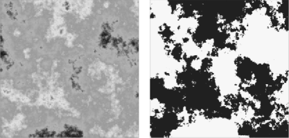
Figure 1: Realization of a stationary centered Gaussian random field $X$ with covariance function $\operatorname{\mathsf{cov}}(X(0),X(t))=\exp(-\|t\|_{2})$ (left figure), bright colours indicate high values of $X$. The excursion set $A_{u}(X,T)$ for $u=0$ is shown in black (right figure).

For a real-valued random field $X=\{X(t),t\in\mathbb{R}^{d}\},$ we assume the measurability of $X(\cdot)$ as a function on $\mathbb{R}^{d}\times\Omega$ endowed with the $\sigma$-algebra $\mathcal{B}(\mathbb{R}^{d})\otimes\mathcal{F}$.

Definition 5.

Let $X$ be a measurable real-valued function on $\mathbb{R}^{d}$ and $T\subset\mathbb{R}^{d}$ be a $($Lebesgue$)$ measurable subset. Then, for each $u\in\mathbb{R,}$

$$A_{u}(X,T)=\{t\in T\colon\ X(t)\geq u\}$$

is called the excursion set of $X$ in $T$ over the level $u$.

Let $\nu_{d}(B)$ be the volume (i.e., the Lebesgue measure) of a measurable set $B\subset\mathbb{R}^{d}$ and $\mathbb{I}\{C\}$ denote the indicator of a set $C$.

Since $X$ is measurable, the volume of the excursion set

$$\nu_{d}(A_{u}(X,T))=\int_{T}\mathbb{I}\{X(t)\geq u\}\,\mathrm{d}t\vspace*{-1pt}$$

is a random variable for each $u\in\mathbb{R}$ and any measurable set $T\subset\mathbb{R}^{d}$.

2.3 Growing sets

Denote the boundary of a set $B\subset\mathbb{R}^{d}$ by $\partial B$. The Minkowski sum of two sets, $A$, $B\subset\mathbb{R}^{d}$, is given by $A\oplus B=\{x+y\colon\ x\in A,y\in B\}$. The following concept of “regular growth” for a family of subsets in $\mathbb{R}^{d}$ will be used in the sequel.

Definition 6.

A sequence, $(W_{n})_{n\in\mathbb{N}}$, of bounded measurable sets, $W_{n}\subset\mathbb{R}^{d}$, tends to infinity in the Van Hove sense $($VH-growing$)$ if, for any ${\varepsilon}>0$, one has

$$\nu_{d}(W_{n})\to\infty\quad\mbox{and}\quad\frac{\nu_{d}(\partial W_{n}\oplus B_{{\varepsilon}}(0))}{\nu_{d}(W_{n})}\to 0\vspace*{-1pt}$$ (7)

as $n\to\infty$, where $B_{{\varepsilon}}(0)=\{x\in\mathbb{R}^{d}\colon\ \|x\|_{2}\leq{\varepsilon}\}$ is the closed ball in $\mathbb{R}^{d}$ with center at the origin $0\in\mathbb{R}^{d}$ and radius ${\varepsilon}$.

If $W_{n}=(a(n),b(n)]=(a_{1}(n),b_{1}(n)]\times\cdots\times(a_{d}(n),b_{d}(n)]$ is a parallelepiped, then $W_{n}\to\infty$ in the Van Hove sense if and only if $b_{k}(n)-a_{k}(n)\to\infty$ as $n\to\infty$ for $k=1,\ldots,d$.

Definition 7.

A sequence of finite sets $U_{n}\subset\mathbb{Z}^{d}$ tends to infinity in a regular way if

$$\frac{\operatorname{\mathsf{card}}\delta U_{n}}{\operatorname{\mathsf{card}}U_{n}}\to 0\qquad\mbox{as }n\to\infty;\vspace*{-1pt}$$ (8)

cf. (7). Here $\delta U_{n}=\{j\in\mathbb{Z}^{d}\setminus U_{n}\colon\ \operatorname{\mathsf{dist}}(j,U_{n})=1\}$ and $\operatorname{\mathsf{dist}}(j,U_{n})=\min_{k\in U_{n}}\|j-k\|_{\infty}$.

3 Central limit theorem

Now we state and prove a CLT for the volume of excursion sets of random fields. Ivanov and Leonenko [12] studied stationary and isotropic Gaussian random fields. In our approach, the isotropy of Gaussian fields is not required. Moreover, we consider a more general class of random fields possessing the quasi-association property. To avoid long formulations, we introduce the following two conditions for a random field $X=\{X(t),t\in\mathbb{R}^{d}\}$. (

• B)]

• $X$ is quasi-associated and strictly stationary such that $X(0)$ has a bounded density. Assume that the covariance function of $X$ is continuous and there exists some $\alpha>3d$ such that

  $$|\operatorname{\mathsf{cov}}(X(0),X(t))|=\mathrm{O}(\|t\|_{2}^{-\alpha})\qquad\mbox{as }\|t\|_{2}\to\infty.\vspace*{-1pt}$$ (9)

• $X$ is Gaussian and stationary. Suppose that its continuous covariance function satisfies (9) for some $\alpha>d$.

Notice that continuity of the covariance function of $X$ implies the existence of a measurable modification of this field. We consider only such versions of $X$. We exclude the trivial case when $X(t)=$ const a.s. for all $t\in\mathbb{R}^{d}$.

3.1 Quasi-associated random fields

To prove the CLT for the volume of excursion sets of a random field satisfying condition (A), we need the following auxiliary result.

Lemma 1 (([7], Lemma 7.3.4))

Let $\{U,V\}\in\mathsf{QA,}$ where random variables $U$ and $V$ are square-integrable and have densities bounded by $a>0$. Then

$$|\operatorname{\mathsf{cov}}(\mathbb{I}\{U\geq u\},\mathbb{I}\{V\geq v\})|\leq 3\cdot 2^{2/3}a^{2/3}|\operatorname{\mathsf{cov}}(U,V)|^{1/3}\vspace*{-1pt}$$

for arbitrary $u,v\in\mathbb{R}$.

Theorem 1

Let $X=\{X(t),t\in\mathbb{R}^{d}\}$ be a random field satisfying condition (A). Then, for any sequence of VH-growing sets $W_{n}\subset\mathbb{R}^{d}$ and each $u\in\mathbb{R}$, one has

$$\frac{\nu_{d}(A_{u}(X,W_{n}))-\nu_{d}(W_{n}){\mathsf{P}}(X(0)\geq u)}{\sqrt{\nu_{d}(W_{n})}}\stackrel{{\scriptstyle d}}{{\rightarrow}}Y_{u}\sim\mathcal{N}(0,\sigma^{2}(u)),\qquad n\to\infty.\vspace*{-1pt}$$ (10)

Here $\stackrel{{\scriptstyle d}}{{\rightarrow}}$ denotes convergence in distribution, $Y_{u}$ being a Gaussian random variable with mean zero and variance

$$\sigma^{2}(u)=\int_{\mathbb{R}^{d}}\operatorname{\mathsf{cov}}\bigl{(}\mathbb{I}\{X(0)\geq u\},\mathbb{I}\{X(t)\geq u\}\bigr{)}\,\mathrm{d}t\in\mathbb{R}_{+}.\vspace*{-1pt}$$ (11)

Proof.

Fix any $u\in\mathbb{R}$ and transform a random field $X$ into a field $Z=\{Z(j),j\in\mathbb{Z}^{d}\},$ setting

$$Z(j)=\int_{Q_{j}}\mathbb{I}\{X(t)\geq u\}\,\mathrm{d}t-{\mathsf{P}}\bigl{(}X(0)\geq u\bigr{)},\vspace*{-1pt}$$ (12)

where the unit cubes

$$Q_{j}=\{x=(x_{1},\ldots,x_{d})^{\top}\in\mathbb{R}^{d}\colon\ 0<x_{k}\leq 1,k=1,\ldots,d\}\oplus\{j\},\qquad j=(j_{1},\ldots,j_{d})^{\top}\in\mathbb{Z}^{d}.$$

The Fubini theorem implies $\mathsf{E}Z(j)=0$ for any $j\in\mathbb{Z}^{d}$. It is easily seen that the field $Z$ is strictly stationary and square-integrable. Introduce

$$J_{n}^{-}=\{j\in\mathbb{Z}^{d}\colon\ Q_{j}\subset W_{n}\},\qquad J_{n}^{+}=\{j\in\mathbb{Z}^{d}\colon\ Q_{j}\cap W_{n}\neq\varnothing\}$$ (13)

and

$$W_{n}^{-}=\bigcup_{j\in J_{n}^{-}}Q_{j},\qquad W_{n}^{+}=\bigcup_{j\in J_{n}^{+}}Q_{j}.$$

Due to (7), we conclude (see [7], Lemma 3.1.2) that

$$\nu_{d}(W_{n}^{-})\to\infty\quad\mbox{and}\quad\nu_{d}(W_{n}^{-})/\nu_{d}(W_{n}^{+})\to 1\qquad\mbox{as }n\to\infty.$$ (14)

Write

$$\frac{\nu_{d}(A_{u}(X,W_{n}))-\nu_{d}(W_{n}){\mathsf{P}}(X(0)\geq u)}{\sqrt{\nu_{d}(W_{n})}}$$

$$\quad=\frac{\nu_{d}(A_{u}(X,W_{n}^{-}))-\nu_{d}(W_{n}^{-}){\mathsf{P}}(X(0)\geq u)}{\sqrt{\nu_{d}(W_{n})}}$$ (15)

$$\qquad{}+\frac{\nu_{d}(A_{u}(X,W_{n}))-\nu_{d}(A_{u}(X,W_{n}^{-}))-(\nu_{d}(W_{n})-\nu_{d}(W_{n}^{-})){\mathsf{P}}(X(0)\geq u)}{\sqrt{\nu_{d}(W_{n})}}.$$

We prove that the second term on the right-hand side in (3.1) tends to zero in probability. By Chebyshev’s inequality, it suffices to show that

$$\operatorname{\mathsf{var}}\bigl{(}\nu_{d}(A_{u}(X,W_{n}))-\nu_{d}(A_{u}(X,W_{n}^{-}))\bigr{)}/\nu_{d}(W_{n})\to 0,\qquad n\to\infty.$$

Set

$$Y_{n}(j)=\int_{Q_{j}\cap W_{n}}\mathbb{I}\{X(t)\geq u\}\,\mathrm{d}t-\nu_{d}(Q_{j}\cap W_{n}){\mathsf{P}}\bigl{(}X(0)\geq u\bigr{)}\qquad\mbox{for }j\in\mathbb{Z}^{d},\ n\in\mathbb{N}.$$

Note that $Y_{n}(j)=Z(j)$ for $j\in J_{n}^{-}$ and $n\in\mathbb{N}$ (clearly $Y_{n}(j)$ and $Z(j)$ depend on $u$ as well). Applying the Fubini theorem and Lemma 1, we get

$$\operatorname{\mathsf{var}}\bigl{(}\nu_{d}(A_{u}(X,W_{n}))-\nu_{d}(A_{u}(X,W_{n}^{-}))\bigr{)}$$

$$\quad=\operatorname{\mathsf{var}}\biggl{(}\sum_{j\in J_{n}^{+}\setminus J_{n}^{-}}Y_{n}(j)\biggr{)}$$

$$\quad\leq\sum_{j,m\in J_{n}^{+}\setminus J_{n}^{-}}\int_{Q_{j}\times Q_{m}}\bigl{|}\operatorname{\mathsf{cov}}\bigl{(}\mathbb{I}\{X(s)\geq u\},\mathbb{I}\{X(t)\geq u\}\bigr{)}\bigr{|}\,\mathrm{d}s\,\mathrm{d}t$$ (16)

$$\quad\leq\nu_{d}(W_{n}^{+}\setminus W_{n}^{-})\sum_{j\in\mathbb{Z}^{d}}\int_{Q_{0}\times Q_{j}}C_{1}|\operatorname{\mathsf{cov}}(X(s),X(t))|^{1/3}\,\mathrm{d}s\,\mathrm{d}t$$

$$\quad\leq\nu_{d}(W_{n}^{+}\setminus W_{n}^{-})\Biggl{(}C_{2}+C_{3}\sum_{r=r_{0}}^{\infty}\sum_{j\in\mathbb{Z}^{d}\colon\ \|j\|_{\infty}=r}\int_{Q_{0}\times Q_{j}}\|s-t\|_{2}^{-\alpha/3}\,\mathrm{d}s\,\mathrm{d}t\Biggr{)}$$

$$\quad\leq\nu_{d}(W_{n}^{+}\setminus W_{n}^{-})\Biggl{(}C_{2}+C_{4}\sum_{r=1}^{\infty}r^{d-1}r^{-\alpha/3}\Biggr{)}=C_{5}\nu_{d}(W_{n}^{+}\setminus W_{n}^{-})$$

for some $r_{0}>0$ and all $n\in\mathbb{N}$. The factors $C_{i}$ do not depend on $n$. We used the inequality $|\operatorname{\mathsf{cov}}(X(s),X(t))|\leq\tau^{2}$ for all $s,t\in\mathbb{R}^{d}$, which is satisfied as $\operatorname{\mathsf{var}}X(t)=\tau^{2}$ for any $t\in\mathbb{R}^{d}$. We also took into account that

$$\operatorname{\mathsf{card}}\{j\in\mathbb{Z}^{d}\colon\ \|j\|_{\infty}=r\}\leq C_{6}r^{d-1}$$

for each $r\in\mathbb{N}$ and employed the inequality (9) with $\alpha>3d$.

By (14), (3.1) and in view of the relation $\nu_{d}(W_{n}^{-})\leq\nu_{d}(W_{n})\leq\nu_{d}(W_{n}^{+}),$ we get

$$\operatorname{\mathsf{var}}\bigl{(}\bigl{(}\nu_{d}(A_{u}(X,W_{n}))-\nu_{d}(A_{u}(X,W_{n}^{-}))\bigr{)}/\sqrt{\nu_{d}(W_{n})}\bigr{)}\to 0,\qquad n\to\infty.$$

Now we show that $J_{n}^{-}$, introduced in (13), tends to infinity in a regular way as $n\to\infty$. Indeed, $J_{n}^{-}\subset J_{n}\subset J_{n}^{+}$, where $J_{n}:=W_{n}\cap\mathbb{Z}^{d}$, $n\in\mathbb{Z}^{d}$. Due to [7], Lemma 3.1.5, $J_{n}$ tends to infinity in a regular way. Thus, it suffices to mention that $\delta J_{n}^{-}\subset\delta J_{n}\cup(J_{n}\setminus J_{n}^{-})$ and apply the relations $\operatorname{\mathsf{card}}\delta J_{n}/\operatorname{\mathsf{card}}J_{n}\to 0$ and $\operatorname{\mathsf{card}}J_{n}^{+}/\operatorname{\mathsf{card}}J_{n}^{-}\to 1$ as $n\to\infty$. Lemma 3.1.6 of [7] implies that $W_{n}^{-}=\bigcup_{j\in J_{n}^{-}}Q_{j}$ tends to infinity in the Van Hove sense as $n\to\infty$.

So, while establishing (10), we can assume w.l.g. that $W_{n}=W_{n}^{-}$, that is, $W_{n}$ is a finite union of cubes $Q_{j}$ $(n\in\mathbb{N})$ and the sequence $(W_{n})_{n\in\mathbb{N}}$ is VH-growing.

Observe that

$$\frac{\nu_{d}(A_{u}(X,W_{n}))-\nu_{d}(W_{n}){\mathsf{P}}(X(0)\geq u)}{\sqrt{\nu_{d}(W_{n})}}=\frac{\sum_{j\in W_{n}\cap\mathbb{Z}^{d}}Z(j)}{\sqrt{\nu_{d}(W_{n})}}:=S_{n}.$$

As $X=\{X(t),t\in\mathbb{R}^{d}\}\in\mathsf{QA}$, it follows from (6) and (9) that $X\in(\mathit{BL},\theta)$ with

$$\theta_{r}(X)=\mathrm{O}(r^{-\alpha+d})\qquad\mbox{as }r\to\infty(r>0).$$

For $\gamma>0$ (and $u$ fixed) introduce the Lipschitz functions $h_{\gamma}\mathchoice{\nobreak\,\colon}{\nobreak\,\colon}{\nobreak\,\colon\;}{\nobreak\,\colon\;}\mathbb{R}\rightarrow\mathbb{R}$ by the formula

$$h_{\gamma}(x)=\cases{\displaystyle 0,&\quad if $x\leq u-\gamma$,\cr\displaystyle(x-u+\gamma)/\gamma,&\quad if $u-\gamma<x\leq u$,\cr\displaystyle 1,&\quad otherwise.}$$ (17)

Superposition of two Lipschitz functions is also a Lipschitz one. Thus, for $n\in\mathbb{N}$ and $\gamma>0$, the random field $Z_{n,\gamma}=\{Z_{n,\gamma}(j),j=(j_{1},\ldots,j_{d})^{\top}\in\mathbb{Z}^{d}\}\in(\mathit{BL},\theta),$ where

$$Z_{n,\gamma}(j)=\frac{1}{n^{d}}\sum_{k_{1},\ldots,k_{d}=1}^{n}h_{\gamma}\biggl{(}X\biggl{(}j_{1}+\frac{k_{1}}{n},\ldots,j_{d}+\frac{k_{d}}{n}\biggr{)}\biggr{)}-{\mathsf{E}}h_{\gamma}(X(0))$$ (18)

and the terms of a sequence $\theta(Z_{n,\gamma})$ admit the estimate

$$\theta_{r}(Z_{n,\gamma})\leq C_{7}\gamma^{-2}r^{-\alpha+d},\qquad r\in\mathbb{N},$$ (19)

with $C_{7}$ depending neither on $\gamma$ nor on $n$.

It is not difficult to verify that the finite-dimensional distributions of the fields $Z_{n,\gamma}$ weakly converge to the corresponding ones of the field $Z_{\gamma}$ as $n\to\infty,$ where

$$Z_{\gamma}(j)=\int_{Q_{j}}h_{\gamma}(X(t))\,\mathrm{d}t-{\mathsf{E}}h_{\gamma}(X(0)),\qquad j\in\mathbb{Z}^{d}.$$ (20)

Consequently (see [7], Lemma 1.5.16), we can claim that $Z_{\gamma}\in(\mathit{BL},\theta)$ and $\theta_{r}(Z_{\gamma})$ is bounded by the right-hand side of inequality (19). Theorem 3.1.12 of [7], guarantees that, for each $\gamma>0$,

$$S_{n}(\gamma):=\frac{\sum_{j\in W_{n}\cap\mathbb{Z}^{d}}Z_{\gamma}(j)}{\sqrt{\nu_{d}(W_{n})}}\stackrel{{\scriptstyle d}}{{\to}}Y_{u,\gamma}\sim\mathcal{N}(0,\sigma^{2}(u,\gamma)),\qquad n\to\infty,$$ (21)

where

$$\sigma^{2}(u,\gamma)=\sum_{j\in\mathbb{Z}^{d}}\operatorname{\mathsf{cov}}(Z_{\gamma}(0),Z_{\gamma}(j))=\int_{\mathbb{R}^{d}}\operatorname{\mathsf{cov}}(h_{\gamma}(X(0)),h_{\gamma}(X(t)))\,\mathrm{d}t\in\mathbb{R}_{+}.$$

Therefore, to prove (10), two steps remain. First of all, we estimate the difference of the characteristic functions of the random variables $S_{n}(\gamma)$ and $S_{n}$ and show that it tends to zero as $\gamma\to 0+$. After that, we verify that

$$\sigma^{2}(u,\gamma)\to\sigma^{2}(u)\qquad\mbox{as }\gamma\to 0+.$$ (22)

Set $h(x)=\mathbb{I}\{x\geq u\}$ and $H_{\gamma}(x)=h_{\gamma}(x)-h(x),$ where $x\in\mathbb{R}$ (and $u\in\mathbb{R}$ is fixed). Then, for each $\lambda\in\mathbb{R}$, one has

$$\bigl{|}\mathsf{E}\mathrm{e}^{\mathrm{i}\lambda S_{n}(\gamma)}-\mathsf{E}\mathrm{e}^{\mathrm{i}\lambda S_{n}}\bigr{|}\leq|\lambda|\mathsf{E}|S_{n}(\gamma)-S_{n}|\leq|\lambda|\biggl{(}\frac{V_{n}(\gamma)}{\nu_{d}(W_{n})}\biggr{)}^{1/2},$$ (23)

where $\mathrm{i}^{2}=-1$ and

$$V_{n}(\gamma)=\mathsf{E}\biggl{(}\sum_{j\in W_{n}\cap\mathbb{Z}^{d}}\int_{Q_{j}}\bigl{(}H_{\gamma}(X(t))-\mathsf{E}H_{\gamma}(X(t))\bigr{)}\,\mathrm{d}t\biggr{)}^{2}.$$

It is easily seen that

$$V_{n}(\gamma)\leq\nu_{d}(W_{n})\int_{\mathbb{R}^{d}}|\operatorname{\mathsf{cov}}(H_{\gamma}(X(0)),H_{\gamma}(X(t)))|\,\mathrm{d}t.$$ (24)

Furthermore, we have

$$|\operatorname{\mathsf{cov}}(H_{\gamma}(X(0)),H_{\gamma}(X(t)))|\leq(\mathsf{E}(H_{\gamma}(X(0)))^{2}\mathsf{E}(H_{\gamma}(X(t)))^{2})^{1/2}\leq a\gamma,$$

where $a$ is a constant that bounds the density of $X(0)$. If $|\operatorname{\mathsf{cov}}(X(0),X(t))|^{1/3}\leq\gamma$, then reasoning similar to that proving Lemma 1 leads to the inequality

$$|\operatorname{\mathsf{cov}}(H_{\gamma}(X(0)),H_{\gamma}(X(t)))|\leq C(a)|\operatorname{\mathsf{cov}}(X(0),X(t))|^{1/3}$$ (25)

with some $C(a)>0$. Write $\alpha=3(d+\mu)$, $\mu>0$, and take $R=c\gamma^{-{1}/({d+\mu})}$, where $c>0$. Then, in view of (9) and due to the appropriate choice of $c$, one can conclude that for all $\gamma>0$ small enough,

$$F(\gamma) := \int_{\mathbb{R}^{d}}|\operatorname{\mathsf{cov}}(H_{\gamma}(X(0)),H_{\gamma}(X(t)))|\,\mathrm{d}t$$

$$\leq a\gamma\omega_{d}R^{d}+C_{8}\int_{\|t\|_{2}\geq R}\|t\|_{2}^{-\alpha/3}\,\mathrm{d}t\leq C_{9}\gamma^{{\mu}/({d+\mu})},$$

where $\omega_{d}=\pi^{d/2}/(\Gamma(d/2+1))$ is the volume of the unit ball in $\mathbb{R}^{d}$ with the Euclidean norm. Consequently, inequalities (23), (24) and (3.1) imply that the laws of $S_{n}(\gamma)$ and $S_{n}$ are close for all $n$ large enough if $\gamma>0$ is small enough.

Next, we proceed to (22). By the arguments leading to (3.1) and invoking Lemma 1, we deduce that $\sigma^{2}(u)<\infty$. Similar to (25), one shows that if $|\operatorname{\mathsf{cov}}(X(s),X(t))|^{1/3}\leq\gamma$, then

$$|\operatorname{\mathsf{cov}}(h(X(s)),H_{\gamma}(X(t)))|\leq D(a)|\operatorname{\mathsf{cov}}(X(s),X(t))|^{1/3}$$ (27)

with $D(a)>0$ depending on $a$ only. The absolute value of $\sigma^{2}(u,\gamma)-\sigma^{2}(u)$ does not exceed the following expression:

$$F(\gamma)+\int_{\mathbb{R}^{d}}|\operatorname{\mathsf{cov}}(h(X(0)),H_{\gamma}(X(t)))|\,\mathrm{d}t+\int_{\mathbb{R}^{d}}|\operatorname{\mathsf{cov}}(H_{\gamma}(X(0)),h(X(t)))|\,\mathrm{d}t.$$

Taking into account the above upper bound and relations (3.1) and (27), we complete the proof of (22). The asymptotic (finite) variances $\sigma^{2}(u,\gamma)$ are non-negative, whence one concludes that $\sigma^{2}(u)\geq 0$.

In view of (21)–(23), the proof is complete. ∎

Now we turn to the multidimensional CLT for random vectors,

$$S_{\vec{u}}(X,W_{n})=(\nu_{d}(A_{u_{1}}(X,W_{n})),\ldots,\nu_{d}(A_{u_{r}}(X,W_{n})))^{\top},\qquad n\in\mathbb{N},$$ (28)

where $\vec{u}=(u_{1},\ldots,u_{r})^{\top}\in\mathbb{R}^{r}$.

Theorem 2

Let $X=\{X(t),t\in\mathbb{R}^{d}\}$ be a random field satisfying condition (A). Then, for each $\vec{u}=(u_{1},\ldots,u_{r})^{\top}\in\mathbb{R}^{r}$ and any VH-growing sequence $(W_{n})_{n\in\mathbb{N}}$ of subsets of $\mathbb{R}^{d}$, one has

$$\nu_{d}(W_{n})^{-1/2}\bigl{(}S_{\vec{u}}(X,W_{n})-\nu_{d}(W_{n})P(\vec{u})\bigr{)}\stackrel{{\scriptstyle d}}{{\rightarrow}}V_{\vec{u}}\sim\mathcal{N}(0,\Sigma(\vec{u}))\qquad\mbox{as }n\to\infty,$$ (29)

where

$$P(\vec{u})=\bigl{(}{\mathsf{P}}\bigl{(}X(0)\geq u_{1}\bigr{)},\ldots,{\mathsf{P}}\bigl{(}X(0)\geq u_{r}\bigr{)}\bigr{)}^{\top}$$

and $\Sigma(\vec{u})=(\sigma_{lm}(\vec{u}))_{l,m=1}^{r}$ is an $(r\times r)$-matrix having the elements

$$\sigma_{lm}(\vec{u})=\int_{\mathbb{R}^{d}}\operatorname{\mathsf{cov}}\bigl{(}\mathbb{I}\{X(0)\geq u_{l}\},\mathbb{I}\{X(t)\geq u_{m}\}\bigr{)}\,\mathrm{d}t.$$ (30)

Proof.

Observe that the convergence of all $r^{2}$ integrals in (30) is proved in the same way as that of the integral representing $\sigma^{2}(u)$ in the one-dimensional case. The result follows by using the Cramér–Wold device. We omit further details that are quite similar to those in the proof of Theorem 1. ∎

The last theorem entails:

Corollary 1.

Let $X=\{X(t),t\in\mathbb{R}^{d}\}$ be a random field satisfying condition (A). Assume that $\Sigma(\vec{u})$ is non-degenerate for some $\vec{u}\in\mathbb{R}^{r}$. Then, for this $\vec{u}$ and any sequence $(W_{n})_{n\in\mathbb{N}}$ of VH-growing subsets of $\mathbb{R}^{d}$, one has

$$\nu_{d}(W_{n})^{-1/2}\Sigma(\vec{u})^{-1/2}\bigl{(}S_{\vec{u}}(X,W_{n})-\nu_{d}(W_{n})P(\vec{u})\bigr{)}\stackrel{{\scriptstyle d}}{{\rightarrow}}V\sim\mathcal{N}(0,\mathrm{I})\qquad\mbox{as }n\to\infty;$$

here I denotes the unit $(r\times r)$-matrix.

3.2 Shot noise random fields

We verify the conditions of Theorem 1 for shot noise random fields. These fields appear naturally in the theory of disordered structures. Let $\mathcal{B}({\mathbb{R}}^{d})$ (resp., $\mathcal{B}_{0}({\mathbb{R}}^{d})$) be the family of all (bounded) Borel sets in ${\mathbb{R}}^{d}$. A shot noise random field $X=\{X(t),t\in{\mathbb{R}}^{d}\}$ is defined by the relation

$$X(t)=\sum_{i\in{\mathbb{N}}}\xi_{i}\varphi(t-x_{i}),$$

where $\{\xi_{i}\}$ is a family of i.i.d. non-negative random variables and $\{x_{i}\}$ is a homogeneous Poisson point process in ${\mathbb{R}}^{d}$ with intensity $\lambda\in(0,\infty)$, that is, $\{x_{i}\}$ is the support set of a random Poisson counting measure $\{N_{B},B\in\mathcal{B}({\mathbb{R}}^{d})\},$ where $N_{B}=\#\{i\colon\ x_{i}\in B\}$ has the following properties: (

• ii)]

• $N_{B_{1}},N_{B_{2}},\ldots$ are independent for pairwise disjoint $B_{1},B_{2},\ldots\in\mathcal{B}_{0}({\mathbb{R}}^{d})$,

• $N_{B}\sim\operatorname{Pois}(\lambda\nu_{d}(B))$ for all $B\in\mathcal{B}_{0}({\mathbb{R}}^{d})$.

Suppose that $\{\xi_{i}\}$, $N_{(\cdot)}$ are independent, ${\mathsf{E}}\xi_{i}^{2}<\infty$ and $\varphi\mathchoice{\nobreak\,\colon}{\nobreak\,\colon}{\nobreak\,\colon\;}{\nobreak\,\colon\;}{\mathbb{R}}^{d}\to{\mathbb{R}}_{+}$ is a Borel function.

For the shot-noise field $X$ introduced above, we impose the condition:

(C) $X(0)$ has a bounded density and for a function $\varphi$ bounded and uniformly continuous on ${\mathbb{R}}^{d},$

$$\varphi(t)\leq\varphi_{0}(\|t\|_{2})=\mathrm{O}(\|t\|_{2}^{-\alpha})\qquad\mbox{as }\|t\|_{2}\to\infty,$$ (31)

where $\alpha>3d$ and $\varphi_{0}\mathchoice{\nobreak\,\colon}{\nobreak\,\colon}{\nobreak\,\colon\;}{\nobreak\,\colon\;}{\mathbb{R}}_{+}\to{\mathbb{R}}_{+}$.

Proposition 1

The statement of Theorem 1 holds for a random field $X$ satisfying condition (C).

Proof.

By [7], Theorem 1.3.8, $X$ is associated and hence quasi-associated. Moreover, it is strictly stationary with covariance function given, for example, in [7], Theorem 2.3.6. The continuity of the covariance function follows from the inequality

$$|\operatorname{\mathsf{cov}}(X(0),X(s))-\operatorname{\mathsf{cov}}(X(0),X(t))|\leq\lambda\mathsf{E}\xi_{1}^{2}\sup_{y\in{\mathbb{R}}^{d}}|\varphi(t-y)-\varphi(s-y)|\int_{{\mathbb{R}}^{d}}|\varphi(y)|\,\mathrm{d}y$$

and the uniform continuity of $\varphi$. Corollary 2.3.7 of [7] yields the desired bound for the covariance function in condition (A). The proof is complete. ∎

Note that the characteristic function of $X(0)$, provided by [7], Lemma 1.3.7, is integrable if

$$\int_{{\mathbb{R}}}\biggl{|}\exp\biggl{\{}\lambda\int_{{\mathbb{R}}^{d}}\bigl{(}\varphi_{\xi}(s\varphi(t))-1\bigr{)}\,\mathrm{d}t\biggr{\}}\biggr{|}\,\mathrm{d}s<\infty.$$ (32)

Thus, (32) guarantees the existence of the bounded density of $X(0)$.

Condition (32) can be easily verified in a number of special cases; for instance, if $\xi_{1}=\operatorname{const}>0$ a.s. and $\varphi(t)=a\exp\{-b\|t\|_{2}\}$ or $\varphi(t)=a\min\{1,\|t\|_{2}^{-b}\}$ with $a,b>0$.

3.3 Gaussian random fields

In contrast to Lemma 1, we obtain a sharper estimate for the covariance of indicator functions in the Gaussian case. Our result extends formula (2.7.1) of [12]. Let $\Phi$ and $\Psi$ stand for the cumulative distribution function and the tail distribution function of a standard Gaussian random variable, respectively.

Lemma 2

Let $(U,V)^{\top}$ be a Gaussian random vector in $\mathbb{R}^{2}$ such that $U\sim\mathcal{N}(a,\tau^{2})$, $V\sim\mathcal{N}(a,\tau^{2}),$ where $a\in\mathbb{R}$, $\tau>0$ and correlation coefficient $\operatorname{\mathsf{corr}}(U,V)=\rho$. Then, for any $u,v\in{\mathbb{R}}$ and $\rho\in(-1,1)$, the following equality holds:

$$\operatorname{\mathsf{cov}}(\mathbb{I}\{U\geq u\},\mathbb{I}\{V\geq v\})$$

(33)

$$\quad=\frac{1}{2\uppi}\int_{0}^{\rho}\frac{1}{\sqrt{1-r^{2}}}\exp\biggl{\{}-\frac{(u-a)^{2}-2r(u-a)(v-a)+(v-a)^{2}}{2\tau^{2}(1-r^{2})}\biggr{\}}\,\mathrm{d}r.$$

In particular, for $u=v$, one has

$$\operatorname{\mathsf{cov}}(\mathbb{I}\{U\geq u\},\mathbb{I}\{V\geq u\})=\frac{1}{2\uppi}\int_{0}^{\rho}\frac{1}{\sqrt{1-r^{2}}}\exp\biggl{\{}-\frac{(u-a)^{2}}{\tau^{2}(1+r)}\biggr{\}}\,\mathrm{d}r.$$

Moreover, for any $u,v\in{\mathbb{R}}$ and $\rho\in[-1,1]$, one has the inequality

$$|\operatorname{\mathsf{cov}}(\mathbb{I}\{U\geq u\},\mathbb{I}\{V\geq v\})|\leq|\rho|/4.$$ (34)

Proof.

Using the transformation $x\mapsto(x-a)/\tau$, $x\in\mathbb{R,}$ we can assume w.l.g. that $U\sim\mathcal{N}(0,1)$ and $V\sim\mathcal{N}(0,1)$. Let $\rho\in(-1,1)$. The probability density

$$f_{U,V}(x,y)=\frac{1}{2\uppi\sqrt{1-\rho^{2}}}\exp\biggl{\{}-\frac{x^{2}-2\rho xy+y^{2}}{2(1-\rho^{2})}\biggr{\}}$$

of the bivariate Gaussian random variable $(U,V)^{\top}$ is invariant under the transformation $x\mapsto-x$ and $y\mapsto-y$, $(x,y)^{\top}\in{\mathbb{R}}^{2}$. Therefore,

$$\operatorname{\mathsf{cov}}(\mathbb{I}\{U\geq u\},\mathbb{I}\{V\geq v\})=\operatorname{\mathsf{cov}}(\mathbb{I}\{U\leq-u\},\mathbb{I}\{V\leq-v\}),\qquad u,v\in{\mathbb{R}}.$$

It is well known (see, e.g., [10], formulae (21.12.5) and (21.12.6)) that

$$f_{U,V}(x,y)=\sum_{k=0}^{\infty}\frac{\Phi^{(k+1)}(x)\Phi^{(k+1)}(y)}{k!}\rho^{k},\qquad x,y\in\mathbb{R},$$

where $\Phi^{(k)}(x)=\mathrm{d}^{k}\Phi(x)/\mathrm{d}x^{k}$ and, for any $u,v\in\mathbb{R}$,

$$\int_{-\infty}^{u}\int_{-\infty}^{v}f_{U,V}(x,y)\,\mathrm{d}x\,\mathrm{d}y=\sum_{k=0}^{\infty}\frac{\Phi^{(k)}(u)\Phi^{(k)}(v)}{k!}\rho^{k}.$$

Hence, for each $u,v\in\mathbb{R}$,

$$\mathsf{E}\mathbb{I}\{U\leq-u\}\mathbb{I}\{V\leq-v\} = \int_{-\infty}^{-u}\int_{-\infty}^{-v}f_{U,V}(x,y)\,\mathrm{d}x\,\mathrm{d}y=\sum_{k=0}^{\infty}\frac{\Phi^{(k)}(-u)\Phi^{(k)}(-v)}{k!}\rho^{k}$$

$$= \Phi(-u)\Phi(-v)+\sum_{k=1}^{\infty}\frac{\Phi^{(k)}(-u)\Phi^{(k)}(-v)}{k!}\rho^{k}$$

$$= \Phi(-u)\Phi(-v)+\int_{0}^{\rho}\sum_{k=0}^{\infty}\frac{\Phi^{(k+1)}(-u)\Phi^{(k+1)}(-v)}{k!}r^{k}\,\mathrm{d}r$$

$$= \Phi(-u)\Phi(-v)+\int_{0}^{\rho}f_{U(r),V(r)}(u,v)\,\mathrm{d}r,$$

where $(U(r),V(r))^{\top}$ is a centered bivariate Gaussian vector with $\mathsf{E}U(r)^{2}=\mathsf{E}V(r)^{2}=1$ and $\operatorname{\mathsf{cov}}(U(r),V(r))=r$. Consequently, we get

$$\operatorname{\mathsf{cov}}(\mathbb{I}\{U\leq-u\},\mathbb{I}\{V\leq-v\}) = \int_{0}^{\rho}f_{U(r),V(r)}(u,v)\,\mathrm{d}r$$

$$= \frac{1}{2\uppi}\int_{0}^{\rho}\frac{1}{\sqrt{1-r^{2}}}\mathrm{e}^{-({u^{2}-2ruv+v^{2}})/({2(1-r^{2})})}\,\mathrm{d}r.$$

Passing to random variables $U$ and $V$ with arbitrary mean $a$ and variance $\tau^{2}>0$ gives the formula (2).

To prove inequality (34) for $\rho\in(-1,1)$, write

$$|\operatorname{\mathsf{cov}}(\mathbb{I}\{U\leq-u\},\mathbb{I}\{V\leq-v\})|\leq\frac{1}{2\uppi}\int_{0}^{|\rho|}\frac{1}{\sqrt{1-r^{2}}}\,\mathrm{d}r\leq\frac{1}{2\uppi}\arcsin|\rho|$$

and notice that $\arcsin|\rho|\leq\uppi|\rho|/2$.

The case $|\rho|=1$ is trivial, as $|\mathsf{P}(A\cap B)-\mathsf{P}(A)\mathsf{P}(B)|\leq 1/4$ for any $A,B\in\mathcal{F}$. ∎

The following result generalizes the corresponding one established in [12] (see page 80), where the isotropy of the Gaussian random field was assumed. A central limit theorem for nonlinear transformations of a homogeneous Gaussian random field was used there.

Theorem 3

Let $X=\{X(t),t\in{\mathbb{R}}^{d}\}$ be a Gaussian stationary random field satisfying condition (B) and $X(0)\sim\mathcal{N}(a,\tau^{2})$. Then, for each $u\in{\mathbb{R}}$ and any sequence of $VH$-growing sets $W_{n}\subset{\mathbb{R}}^{d}$, one has

$$\frac{\nu_{d}(A_{u}(X,W_{n}))-\nu_{d}(W_{n})\Psi((u-a)/\tau)}{\sqrt{\nu_{d}(W_{n})}}\stackrel{{\scriptstyle d}}{{\rightarrow}}Y_{u}\sim\mathcal{N}(0,\sigma^{2}(u))$$

as $n\to\infty$. The variance $\sigma^{2}(u)$ introduced in (11) can be written in the following form:

$$\sigma^{2}(u)=\frac{1}{2\uppi}\int_{{\mathbb{R}}^{d}}\int_{0}^{\rho(t)}\frac{1}{\sqrt{1-r^{2}}}\exp\biggl{\{}-\frac{(u-a)^{2}}{\tau^{2}(1+r)}\biggr{\}}\,\mathrm{d}r\,\mathrm{d}t,$$ (35)

where $\rho(t)=\operatorname{\mathsf{corr}}(X(0),X(t))$. In particular,

$$\sigma^{2}(a)=\frac{1}{2\uppi}\int_{{\mathbb{R}}^{d}}\arcsin(\rho(t))\,\mathrm{d}t.\vspace*{-3pt}$$

Proof.

For the Gaussian field $X,$ we have ${\mathsf{P}}(X(0)\geq u)=\Psi((u-a)/\tau)$. Now we apply the upper bound (34) to obtain $|\operatorname{\mathsf{cov}}(X(0),X(t))|$ instead of $|\operatorname{\mathsf{cov}}(X(0),X(t))|^{1/3}$ in the estimates used in the proof of Theorem 1. This leads to the hypothesis that $\alpha>d$ in (9), whereas in condition (A) we assumed $\alpha>3d$. Note that Gaussian fields are quasi-associated [20].

Finally, we express $\sigma^{2}(u)$ (see (11)) in terms of the covariance function of $X$ as in the proof of Lemma 2, and this yields (35). The proof is complete. ∎

Theorem 4

Let $X=\{X(t),t\in{\mathbb{R}}^{d}\}$ be a random field satisfying condition (B) and $X(0)\sim\mathcal{N}(a,\tau^{2})$. Then, for each $\vec{u}=(u_{1},\ldots,u_{r})^{\top}\in{\mathbb{R}}^{r}$ and any sequence $(W_{n})_{n\in{\mathbb{N}}}$ of VH-growing subsets of $\mathbb{R}^{d}$, one has

$$\nu_{d}(W_{n})^{-1/2}\bigl{(}S_{\vec{u}}(X,W_{n})-\nu_{d}(W_{n})\Psi(\vec{u})\bigr{)}\stackrel{{\scriptstyle d}}{{\rightarrow}}V_{\vec{u}}\sim\mathcal{N}(0,\Sigma(\vec{u}))\qquad\mbox{as }n\to\infty.$$ (36)

Here, $\Psi(\vec{u})=(\Psi((u_{1}-a)/\tau),\ldots,\Psi((u_{r}-a)/\tau))^{\top}$ and $\Sigma(\vec{u})=(\sigma_{lm}(\vec{u}))_{l,m=1}^{r}$ is a matrix having the elements

$$\sigma_{lm}(\vec{u})=\frac{1}{2\uppi}\int_{{\mathbb{R}}^{d}}\int_{0}^{\rho(t)}g(r)\,\mathrm{d}r\,\mathrm{d}t,$$ (37)

where

$$g(r)=\frac{1}{\sqrt{1-r^{2}}}\exp\biggl{\{}-\frac{(u_{l}-a)^{2}-2r(u_{l}-a)(u_{m}-a)+(u_{m}-a)^{2}}{2\tau^{2}(1-r^{2})}\biggr{\}}$$

and $\rho(t)=\operatorname{\mathsf{corr}}(X(0),X(t))$. If $\Sigma(\vec{u})$ is non-degenerate, we obtain by virtue of $(\ref{eq:multiclt2})$

$$\nu_{d}(W_{n})^{-1/2}\Sigma(\vec{u})^{-1/2}\bigl{(}S_{\vec{u}}(X,W_{n})-\nu_{d}(W_{n})\Psi(\vec{u})\bigr{)}\stackrel{{\scriptstyle d}}{{\rightarrow}}\mathcal{N}(0,\mathrm{I}),\qquad n\to\infty,$$

where I is the unit $(r\times r)$-matrix.

Proof.

Employing Lemma 2, one can repeat the reasoning proving Theorem 2. Clearly, ${\mathsf{P}}(X(0)\geq u_{l})=\Psi((u_{l}-a)/\tau)$, $l=1,\ldots,r$. The matrix elements $\sigma_{lm}(\vec{u})$ for $l,m=1,\ldots,r$ can be calculated by way of (2). ∎

Formulae in the isotropic case

For the isotropic case, we use the change of variables (passing from $t=(t_{1},\ldots,t_{d})^{\top}$ to spherical coordinates) in integrals (35) and (37) to obtain the following statement.

Corollary 2.

Let the random field $X=\{X(t),t\in{\mathbb{R}}^{d}\}$ satisfying the conditions of Theorem 3 be isotropic $(d\geq 2)$. Then

$$\sigma^{2}(u)=\frac{\mathrm{d}\omega_{d}}{2\uppi}\int_{0}^{\infty}v^{d-1}\int_{0}^{\rho(v)}\frac{1}{\sqrt{1-r^{2}}}\exp\biggl{\{}-\frac{(u-a)^{2}}{\tau^{2}(1+r)}\biggr{\}}\,\mathrm{d}r\,\mathrm{d}v,$$

where $\rho(v)=\operatorname{\mathsf{corr}}(X(0),X(t))$ if $|t|=v$. For $u=a,$ one has

$$\sigma^{2}(a)=\frac{\mathrm{d}\omega_{d}}{2\uppi}\int_{0}^{\infty}v^{d-1}\arcsin(\rho(v))\,\mathrm{d}v.$$

In the multivariate case, (37) can be written as follows:

$$\sigma_{lm}(\vec{u})=\frac{\mathrm{d}\omega_{d}}{2\uppi}\int_{0}^{\infty}v^{d-1}\int_{0}^{\rho(v)}g(r)\,\mathrm{d}r\,\mathrm{d}v$$

for $l,m=1,\ldots,r$.

4 Statistical version of the CLT

Now we provide a statistical version of the CLT involving random self-normalization. Let $r\in{\mathbb{N}}$ be the number of levels to observe.

Theorem 5

Let $X=\{X(t),t\in{\mathbb{R}}^{d}\}$ be a random field satisfying condition (A). Let $u_{k}\in{\mathbb{R}}$, $k=1,\ldots,r$ and $(W_{n})_{n\in{\mathbb{N}}}$ be a sequence of VH-growing sets. Furthermore, let $\hat{C}_{n}=(\hat{c}_{nlm})_{l,m=1}^{r}$ be statistical estimates for non-degenerate asymptotic covariance matrix $\Sigma$ with elements $\sigma_{lm}$ given by (30). Assume that $\hat{c}_{nlm}\stackrel{{\scriptstyle p}}{{\rightarrow}}\sigma_{lm}$ as $n\to\infty$ for any $l,m=1,\ldots,r,$ where $\stackrel{{\scriptstyle p}}{{\rightarrow}}$ denotes convergence in probability. Then

$$\hat{C}_{n}^{-1/2}\nu_{d}(W_{n})^{-1/2}\bigl{(}S(W_{n})-\nu_{d}(W_{n})P(\vec{u})\bigr{)}\stackrel{{\scriptstyle d}}{{\rightarrow}}\mathcal{N}(0,\mathrm{I})\qquad\mbox{as }n\to\infty.\vspace*{-2pt}$$

Proof.

It suffices to use Theorem 2 and elementary properties of the convergence in probability and in law for random vectors. ∎

One feasible estimator for the asymptotic covariance matrix $\Sigma$ that arose in the multivariate CLT, see Theorem 2, can be called a subwindow estimator [18] and is constructed as follows. Let $(V_{n})_{n\in{\mathbb{N}}}$ and $(W_{n})_{n\in{\mathbb{N}}}$ be sequences of VH-growing sets (not necessarily rectangles) such that $V_{n}\subset W_{n}$, $n\geq 1$. Consider $N(n)$ subwindows $V_{n,1},\ldots,V_{n,N(n)}$, where $(N(n))_{n\in{\mathbb{N}}}$ is an increasing sequence of integers with $\lim_{n\to\infty}N(n)=\infty$, and $V_{n,j}=V_{n}\oplus\{h_{n,j}\}$ are subwindows that are translated by certain vectors $h_{n,j}\in{\mathbb{R}}^{d}$, $j=1,\ldots,N(n)$. Assume that $\bigcup_{j=1}^{N(n)}V_{n,j}\subseteq W_{n}$ for each $n\in{\mathbb{N}}$ and there exists some $r>0$ such that

$$V_{n,j}\cap V_{n,i}\subset\partial V_{n,j}\oplus B_{r}(0)\qquad\mbox{for }i,j\in\{1,\ldots,N(n)\}\mbox{ with }i\neq j.\vspace*{-2pt}$$

Denote by

$$\hat{\mu}^{(j)}_{nk}=\frac{1}{\nu_{d}(V_{n})}\int_{V_{n,j}}\mathbb{I}\{X(t)\geq u_{k}\}\,\mathrm{d}t,\qquad j=1,\ldots,N(n),\vspace*{-2pt}$$

the estimator of $\mu_{k}={\mathsf{P}}(X(0)\geq u_{k})$ based on observations within $V_{n,j}$, and by

$$\bar{\mu}_{nk}=\frac{1}{N(n)}\sum_{j=1}^{N(n)}\hat{\mu}^{(j)}_{nk},\qquad n\in\mathbb{N},\ k=1,\ldots,r,\vspace*{-2pt}$$

the average of these estimators. After all, we define the estimator $\hat{\Sigma}_{n}=(\hat{\sigma}_{nlm})_{l,m=1}^{r}$ for the covariance matrix $\Sigma$. Set

$$\hat{\sigma}_{nlm}=\frac{\nu_{d}(V_{n})}{N(n)-1}\sum_{j=1}^{N(n)}\bigl{(}\hat{\mu}^{(j)}_{nl}-\bar{\mu}_{nl}\bigr{)}\bigl{(}\hat{\mu}^{(j)}_{nm}-\bar{\mu}_{nm}\bigr{)}.\vspace*{-2pt}$$ (38)

We recall the following result.

Theorem 6 (([18], Theorem 3))

Let $X=\{X(t),t\in{\mathbb{R}}^{d}\}$ be a strictly stationary random field such that

$$\int_{{\mathbb{R}}^{3d}}\bigl{|}c_{lm}^{(2,2)}(x,y,z)\bigr{|}\,\mathrm{d}x\,\mathrm{d}y\,\mathrm{d}z<\infty,\qquad l,m=1,\ldots,r,\vspace*{-2pt}$$ (39)

where the fourth-order cumulant function

$$c_{lm}^{(2,2)}(x,y,z) = {\mathsf{E}}\bigl{(}[Z_{l}(0)-\mu_{l}][Z_{m}(x)-\mu_{m}][Z_{l}(y)-\mu_{l}][Z_{m}(z)-\mu_{m}]\bigr{)}$$

$${}-\operatorname{\mathsf{cov}}_{lm}(x)\operatorname{\mathsf{cov}}_{lm}(z-y)-\operatorname{\mathsf{cov}}_{ll}(y)\operatorname{\mathsf{cov}}_{mm}(x-z)-\operatorname{\mathsf{cov}}_{lm}(z)\operatorname{\mathsf{cov}}_{ml}(x-y)\vspace*{-2pt}$$

and $\operatorname{\mathsf{cov}}_{lm}(t)=\operatorname{\mathsf{cov}}(\mathbb{I}\{X(0)\geq u_{l}\},\mathbb{I}\{X(t)\geq u_{m}\})$, $l,m=1,\ldots,r$. Then $\hat{\Sigma}$ introduced in (38) is mean-square consistent.

Relation (39) holds for a random field $X$ with finite dependence range. In this case, the estimator $\hat{\Sigma}_{n}$ is mean-square consistent. Among other estimators for the asymptotic covariance matrix, there are two worth mentioning. One estimator that, under certain assumptions, meets the conditions of Theorem 5 is introduced in [8, 6] and involves local averaging. A major disadvantage is tedious calculation in the case of a large observation window. The same problem arises for an estimator based on the covariance function estimation for the underlying random field; see [18] (cf. [12], Chapter 4).

5 Discussion

A very important issue for applications of the estimator $\hat{\Sigma}_{n}$ is the choice of an appropriate size of the (e.g., rectangular) subwindow $V_{n}$. The subwindow size is related to both the covariance structure of the considered random field and the size of the observation window. We will discuss these problems while considering a simple example. The data used consist of $100$ mutually independent realizations of stationary and centered Gaussian random field $X$ with covariance function

$$\operatorname{\mathsf{cov}}(X(0),X(t))=\biggl{(}1-\frac{3\|t\|_{2}}{2a}+\frac{\|t\|_{2}^{3}}{2a^{3}}\biggr{)}\mathbb{I}\{\|t\|_{2}\in[0,a]\},\qquad t\in{\mathbb{R}}^{2},$$

for some $a>0$ according to the spherical covariance model (see [21], page 244), which is often applied in geostatistics. The correlation range $a$ in our simulation study has to be small enough in comparison with the size of the observation window to make the CLT argument work. Here, we take, for example, $a=10$. The fields are simulated in the observation window $W=[0,2000)\times[0,2000)$ on the grid with mesh size one. That means every realization provides $4$ million data points. To generate level sets, we consider the thresholds $u_{1}=-1.0$, $u_{2}=0.0$ and $u_{3}=1.0$. Then

$$\Sigma=\pmatrix{4.6432&&\cr 5.9938&10.5564&\cr 2.7962&5.9938&4.6432}.$$

An appropriate subwindow size can be found focusing only on the threshold $u_{2}=0.0$, since for other threshold values the obtained results differ from this one only slightly. The estimator provides the best result for $\Sigma$ as the edge length of the rectangular subwindow equals $15$. In general, the optimal choice of this length is an open non-trivial problem. After this preliminary step, we are able to apply the subwindow estimator to the simulated data. The following two matrices show averaged estimation results for $\Sigma$ by means of $\hat{\Sigma}$. On the left-hand side, the averaged value of each estimated matrix element is computed out of 100 samples. On the right-hand side, the mean error to the theoretical value is provided.

$$\frac{1}{100}\sum_{k=1}^{100}\hat{\Sigma}_{k}=\pmatrix{\displaystyle 4.6556&&\cr\displaystyle 5.9710&10.5524&\cr\displaystyle 2.8156&5.9934&4.6762\cr},\qquad\mathrm{ME}=\pmatrix{\displaystyle 0.27\%&&\cr\displaystyle-0.38\%&-0.04\%&\cr\displaystyle 0.69\%&\approx 0.00\%&0.71\%\cr}.$$

It would be interesting to propose a statistical hypothesis test based on the established statistical version of the CLT in order to apply it to data concerning the paper production. We will deal with this topic in a separate paper.

6 Open problems

The research area of limit theorems for level sets of random surfaces still offers an abundance of open problems. Let us mention just a few. It would be desirable to prove limit theorems for joint distributions of various surface characteristics of different classes of random fields. For instance, one could consider stable fields. Further on, one can study random fields possessing more strong dependence structure; for example, satisfying condition (A) with $\alpha\leq d$. In this case, the normalizing factors have to be changed and the limiting distributions can be non-Gaussian. Certain results for problems of this type can be found in [12, 15]. One could also prove a functional limit theorem for an innumerable set of thresholds. As our main result could also be called the CLT for the first Minkowski functional, it might be of interest to prove limit theorems involving other Minkowski functionals for level sets such as the boundary length or the Euler characteristics. It is worth mentioning that, for a stationary two-dimensional Gaussian field, this has already been done for the second Minkowski functional in [14].

References

- [1] {bbook}[mr] \bauthor\bsnmAdler, \bfnmRobert J.\binitsR.J. (\byear1981). \btitleThe Geometry of Random Fields. \baddressChichester: \bpublisherWiley. \bidmr=0611857 \endbibitem
- [2] {bbook}[mr] \bauthor\bsnmAdler, \bfnmRobert J.\binitsR.J. &\bauthor\bsnmTaylor, \bfnmJonathan E.\binitsJ.E. (\byear2007). \btitleRandom Fields and Geometry. \baddressNew York: \bpublisherSpringer. \bidmr=2319516 \endbibitem
- [3] {bincollection}[auto:STB—2011-03-03—12:04:44] \bauthor\bsnmBelyaev, \bfnmYu.\binitsY. (\byear1972). \btitleThe general formulae for the mean number of crossings for random processes and fields. In \bbooktitleBursts of Random Fields \bpages38–45. \baddressMoscow: \bpublisherMoscow Univ. Press. \bnote(In Russian.) \endbibitem
- [4] {barticle}[mr] \bauthor\bsnmBrown, \bfnmPatrick E.\binitsP.E., \bauthor\bsnmDiggle, \bfnmPeter J.\binitsP.J. &\bauthor\bsnmHenderson, \bfnmRobin\binitsR. (\byear2003). \btitleA non-Gaussian spatial process model for opacity of flocculated paper. \bjournalScand. J. Statist. \bvolume30 \bpages355–368. \biddoi=10.1111/1467-9469.00335, issn=0303-6898, mr=1983130 \endbibitem
- [5] {bincollection}[mr] \bauthor\bsnmBulinski, \bfnmAlexander\binitsA. (\byear2010). \btitleCentral limit theorem for random fields and applications. In \bbooktitleAdvances in Data Analysis. \bseriesStat. Ind. Technol. \bpages141–150. \baddressBoston, MA: \bpublisherBirkhäuser. \biddoi=10.1007/978-0-8176-4799-5_13, mr=2641266 \endbibitem
- [6] {barticle}[mr] \bauthor\bsnmBulinski, \bfnmAlexander\binitsA. &\bauthor\bsnmKryzhanovskaya, \bfnmNatalya\binitsN. (\byear2006). \btitleConvergence rate in CLT for vector-valued random fields with self-normalization. \bjournalProbab. Math. Statist. \bvolume26 \bpages261–281. \bidissn=0208-4147, mr=2325308 \endbibitem
- [7] {bbook}[auto:STB—2011-03-03—12:04:44] \bauthor\bsnmBulinski, \bfnmA. V.\binitsA.V. &\bauthor\bsnmShashkin, \bfnmA. P.\binitsA.P. (\byear2007). \btitleLimit Theorems for Associated Random Fields and Related Systems. \baddressSingapore: \bpublisherWorld Scientific. \endbibitem
- [8] {barticle}[auto:STB—2011-03-03—12:04:44] \bauthor\bsnmBulinskiĭ, \bfnmA. V.\binitsA.V. (\byear2004). \btitleA statistical version of the central limit theorem for vector-valued random fields. \bjournalMath. Notes \bvolume76 \bpages455–464. \endbibitem
- [9] {barticle}[mr] \bauthor\bsnmBulinskiĭ, \bfnmA. V.\binitsA.V. &\bauthor\bsnmShabanovich, \bfnmÈ.\binitsÈ. (\byear1998). \btitleAsymptotic behavior of some functionals of positively and negatively dependent random fields. \bjournalFundam. Prikl. Mat. \bvolume4 \bpages479–492. \bidissn=1560-5159, mr=1801168 \endbibitem
- [10] {bbook}[mr] \bauthor\bsnmCramér, \bfnmHarald\binitsH. (\byear1946). \btitleMathematical Methods of Statistics. \bseriesPrinceton Mathematical Series \bvolume9. \baddressPrinceton, NJ: \bpublisherPrinceton Univ. Press. \bidmr=0016588 \endbibitem
- [11] {bbook}[mr] \bauthor\bsnmFeller, \bfnmWilliam\binitsW. (\byear1971). \btitleAn Introduction to Probability Theory and Its Applications. Vol. II, \bedition2nd ed. \baddressNew York: \bpublisherWiley. \bidmr=0270403 \endbibitem
- [12] {bbook}[mr] \bauthor\bsnmIvanov, \bfnmA. V.\binitsA.V. &\bauthor\bsnmLeonenko, \bfnmN. N.\binitsN.N. (\byear1989). \btitleStatistical Analysis of Random Fields. \bseriesMathematics and Its Applications (Soviet Series) \bvolume28. \baddressDordrecht: \bpublisherKluwer. \bidmr=1009786 \endbibitem
- [13] {barticle}[mr] \bauthor\bsnmJoag-Dev, \bfnmKumar\binitsK. &\bauthor\bsnmProschan, \bfnmFrank\binitsF. (\byear1983). \btitleNegative association of random variables, with applications. \bjournalAnn. Statist. \bvolume11 \bpages286–295. \biddoi=10.1214/aos/1176346079, issn=0090-5364, mr=0684886 \endbibitem
- [14] {barticle}[mr] \bauthor\bsnmKratz, \bfnmMarie F.\binitsM.F. &\bauthor\bsnmLeón, \bfnmJosé R.\binitsJ.R. (\byear2001). \btitleCentral limit theorems for level functionals of stationary Gaussian processes and fields. \bjournalJ. Theoret. Probab. \bvolume14 \bpages639–672. \biddoi=10.1023/A:1017588905727, issn=0894-9840, mr=1860517 \endbibitem
- [15] {bbook}[auto:STB—2011-03-03—12:04:44] \bauthor\bsnmLeonenko, \bfnmN.\binitsN. (\byear1990). \btitleLimit Theorems for Random Fields with Singular Spectrum. \baddressDordrecht: \bpublisherKluwer. \endbibitem
- [16] {barticle}[auto:STB—2011-03-03—12:04:44] \bauthor\bsnmLeonenko, \bfnmN. N.\binitsN.N. (\byear1987). \btitleLimit distributions of the characteristics of exceeding of a level by a Gaussian random field. \bjournalMath. Notes \bvolume41 \bpages339–345. \endbibitem
- [17] {barticle}[mr] \bauthor\bsnmLeonenko, \bfnmN. N.\binitsN.N. (\byear1988). \btitleSharpness of the normal approximation of functionals of strongly correlated Gaussian random fields. \bjournalMath. Notes \bvolume43 \bpages161–171. \biddoi=10.1007/BF01152556, issn=0025-567X, mr=0939529 \endbibitem
- [18] {barticle}[mr] \bauthor\bsnmPantle, \bfnmUrsa\binitsU., \bauthor\bsnmSchmidt, \bfnmVolker\binitsV. &\bauthor\bsnmSpodarev, \bfnmEvgeny\binitsE. (\byear2010). \btitleOn the estimation of integrated covariance functions of stationary random fields. \bjournalScand. J. Stat. \bvolume37 \bpages47–66. \biddoi=10.1111/j.1467-9469.2009.00663.x, issn=0303-6898, mr=2675939 \endbibitem
- [19] {barticle}[mr] \bauthor\bsnmPitt, \bfnmLoren D.\binitsL.D. (\byear1982). \btitlePositively correlated normal variables are associated. \bjournalAnn. Probab. \bvolume10 \bpages496–499. \bidissn=0091-1798, mr=0665603 \endbibitem
- [20] {barticle}[mr] \bauthor\bsnmShashkin, \bfnmA. P.\binitsA.P. (\byear2002). \btitleQuasi-associatedness of a Gaussian system of random vectors. \bjournalRuss. Math. Surv. \bvolume57 \bpages1243–1244. \biddoi=10.1070/RM2002v057n06ABEH000591, issn=0042-1316, mr=1991881 \endbibitem
- [21] {bbook}[auto:STB—2011-03-03—12:04:44] \bauthor\bsnmWackernagel, \bfnmH.\binitsH. (\byear1998). \btitleMultivariate Geostatistics. \baddressBerlin: \bpublisherSpringer. \endbibitem