Positioning in a flat two-dimensional space-time: the delay master equation

Abstract

The basic theory on relativistic positioning systems in a two-dimensional space-time has been presented in two previous papers [Phys. Rev. D 73, 084017 (2006); 74, 104003 (2006)], where the possibility of making relativistic gravimetry with these systems has been analyzed by considering specific examples. Here we study generic relativistic positioning systems in the Minkowski plane. We analyze the information that can be obtained from the data received by a user of the positioning system. We show that the accelerations of the emitters and of the user along their trajectories are determined by the sole knowledge of the emitter positioning data and of the acceleration of only one of the emitters. Moreover, as a consequence of the so called master delay equation, the knowledge of this acceleration is only required during an echo interval, i.e., the interval between the emission time of a signal by an emitter and its reception time after being reflected by the other emitter. We illustrate these results with the obtention of the dynamics of the emitters and of the user from specific sets of data received by the user.

I Introduction

A relativistic positioning system is defined by four clocks $\gamma_{A}$ (emitters) in arbitrary motion broadcasting their proper times $\tau^{A}$ in some region of a (four-dimensional) space-time coll-1 ; cfm-a ; cfm-b ; coll-pozo-1 ; Minko . Then, every event reached by the signals is naturally labeled by the four times $\{\tau^{A}\}:$ the emission coordinates of this event. The first to propose such physical construction of emission coordinates seem to have been B. Coll coll-2 . Up-to-date references on this concept and its applications and a brief report on relativistic positioning can be found in white .

Although some explicit results have been obtained for generic four-dimensional relativistic positioning coll-pozo-1 ; Minko ; pozo ; bini ; NosERE08 ; Pacome , a full development of the theory requires a previous training on simple and particular situations. A two-dimensional approach to relativistic positioning systems allows the use of precise and explicit diagrams which improve the qualitative comprehension of general four-dimensional positioning systems. The basic features of this two-dimensional approach and the explicit relation between emission coordinates and any given null coordinate system has been presented in cfm-a . There, we have also studied in detail the positioning system defined in flat space-time by geodesic emitters.

In a subsequent work cfm-b we have studied the possibility of making relativistic gravimetry or, more generally, the possibility of obtaining the dynamics of the emitters and/or of the user, as well as the detection of the absence or presence of a gravitational field and its measure. This possibility is examined by means of a (non geodesic) stationary positioning system constructed in two different scenarios: Minkowski and Schwarzschild planes.

In this work we go further in the analysis of two-dimensional positioning problems. Until now cfm-b we have considered stationary or geodesic positioning systems in which the user had, a priory, a partial or full information about the gravitational field and a partial or full information about the positioning system. Here we consider a new situation: the user knows the space-time where he is immersed (flat, Schwarzschild,…) but he has no information about the positioning system. Can the data received by the user determine the characteristics of the positioning system? Can the user obtain information on his local units of time and distance and on his acceleration?

The answer to these questions is still an open problem for a generic space-time, but in this work we undertake this query for Minkowski plane and we analyze the minimum set of data that determine all the user and system information. A remarkable result is that the data received by a user of the positioning system are not independent quantities because of they are submitted to what we call the public data constraints. A consequence of these constraints is the delay master equation which implies that the accelerations of the emitters and of the user along their trajectories are determined by the sole knowledge of the emitter positioning data and of the acceleration of only one of the emitters and only during a (causal) echo interval, i.e., the interval between the emission time of a signal by an emitter and its reception time after being reflected by the other emitter.

In order to better understand our results we illustrate them with two specific situations, the positioning systems defined, respectively, by two inertial emitters or by two (stationary) uniformly accelerated emitters. In them, starting from a partial set of user data, we obtain the proper time and acceleration of the user and we determine the full dynamical properties of the positioning system.

The work is organized as follows. In Sec. II we summarize the basic concepts and notation about relativistic positioning systems in a two-dimensional space-time. In Sec. III we obtain some constraint conditions which restrict the user data and show that all the user and system information can be obtained from the emitter positioning data and the acceleration of only one of the emitters. Sec. IV and Sec. V are devoted to illustrate these general results by considering the above mentioned particular situations. In Sec. VI we deduce stronger restrictions on the user data, the delay master equation, and we clarify the role that this equation plays by applying it to the positioning systems considered before. We finish in Sec. VII with a short discussion about the present results and comments on prospective work.

A short communication of some results of this work was presented in the Spanish Relativity meeting ERE-2007 ere2007 .

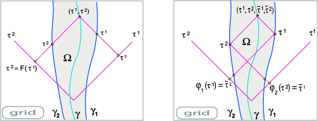
Figure 1: (a) Geometric interpretation of the emission coordinates: the proper times $\{\tau^{1},\tau^{2}\}$ received by a user $\gamma$ give his emission coordinates. These user positioning data $\{\tau^{1},\tau^{2}\}$ allow the user to know his trajectory $\tau^{2}=F(\tau^{1})$ in emission coordinates and he can draw it in the grid $\{\tau^{1}\}\times\{\tau^{2}\}$. (b) The emitter positioning data $\{\tau^{1},\tau^{2};\bar{\tau}^{1},\bar{\tau}^{2}\}$ allow the user to know the emitter trajectories $\varphi_{1}(\tau^{1})$, $\varphi_{2}(\tau^{2})$ in emission coordinates.

II Two-dimensional approach

In a two-dimensional space-time, a relativistic positioning system is defined by two clocks, with world lines $\gamma_{1}$ and $\gamma_{2}$ (emitters), broadcasting their proper times $\tau^{1}$ and $\tau^{2}$ by mean of electromagnetic signals. In the region $\Omega$ between both emitters, the past light cone of every event cuts the emitter world lines at $\gamma_{1}(\tau^{1})$ and $\gamma_{2}(\tau^{2})$, respectively. Then $\{\tau^{1},\tau^{2}\}$ are the emission coordinates of the event: the two proper time signals received by any observer at the event from the two clocks (see Fig. 1(a)). Nevertheless, the signals $\tau^{1}$ and $\tau^{2}$ do not constitute coordinates for the events in the outside region cfm-a .

The plane $\{\tau^{1}\}\times\{\tau^{2}\}$ ($\tau^{1},\tau^{2}\in\mathbb{R}$) in which the different data of the positioning system can be transcribed is the grid of the positioning system. In this grid, the trajectories of the two emitters define an interior region and two exterior ones. This interior region in the grid is in one-to-one correspondence with the interior region in the space-time, i.e. with the set $\Omega$ of events that can be distinguished by the pair of times $(\tau^{1},\tau^{2})$ that reach them. But the exterior regions in the grid have no physical meaning (see cfm-b for more details on the grid).

An observer $\gamma,$ traveling throughout an emission coordinate domain $\Omega$ and equipped with a receiver reading the received proper times $(\tau^{1},\tau^{2})$ at each point of his trajectory, is called a user of the positioning system.

We consider in this work auto-locating positioning systems, which are systems in which every emitter clock not only broadcasts its proper time but also the proper time that it receives from the other. Thus, the physical components of an auto-locating positioning system are cfm-a :

a spatial segment constituted by two emitters $\gamma_{1}$, $\gamma_{2}$ broadcasting their proper times $\tau^{1},$ $\tau^{2}$ and the proper times $\bar{\tau}^{2}$, $\bar{\tau}^{1}$ that they receive each one from the other, and

a user segment constituted by the set of all users traveling in an internal domain $\Omega$ and receiving these four broadcast times $\{\tau^{1},\tau^{2};\bar{\tau}^{1},\bar{\tau}^{2}\}$.

Any user receiving continuously the user positioning data $\{\tau^{1},\tau^{2}\}$ can extract the equation $F$ of his trajectory in the grid (see Fig. 1(a)):

$$\tau^{2}=F(\tau^{1})\,.$$ (1)

On the other hand, any user receiving continuously the emitter positioning data $\{\tau^{1},\tau^{2};\bar{\tau}^{1},\bar{\tau}^{2}\}$ may extract from them not only the equation (1) of his trajectory, but also the equations of the trajectories of the emitters in the grid (see Fig. 1(b)):

$$\varphi_{1}(\tau^{1})=\bar{\tau}^{2}\,,\qquad\varphi_{2}(\tau^{2})=\bar{\tau}^{1}\,.$$ (2)

Eventually, the emitters $\gamma_{1}$, $\gamma_{2}$ could carry accelerometers and broadcast their acceleration $\alpha_{1}$, $\alpha_{2}$, meanwhile the users $\gamma$ could be endowed with receivers able to read the broadcast emitter accelerations $\{\alpha_{1},\alpha_{2}\}$. These new elements allow any user to know the acceleration scalar of the emitters:

$$\alpha_{1}=\alpha_{1}(\tau^{1})\,,\qquad\alpha_{2}=\alpha_{2}(\tau^{2})\,.$$ (3)

Users can also generate their own data, carrying a clock to measure their proper time $\tau$ and/or an accelerometer to measure their proper acceleration $\alpha$. The user’s clock allows any user to know his proper time function $\tau(\tau^{1})$ (or $\tau(\tau^{2})$) and, consequently by using (1), to obtain the proper time parametrization of his trajectory:

$$\gamma\equiv\{\,\tau^{1}=\psi^{1}(\tau)\,;\ \tau^{2}=\psi^{2}(\tau)\}\,.$$ (4)

The user’s accelerometer allows any user to know his proper acceleration scalar:

$$\alpha=\alpha(\tau)\,.$$

Thus, a relativistic positioning system may generate the user data:

$$\{\tau^{1},\tau^{2};\bar{\tau}^{1},\bar{\tau}^{2};\alpha_{1},\alpha_{2};\tau,\alpha\}\,.$$ (5)

The emitter trajectories (2) and the emitter accelerations (3) do not depend on the user that receives them. Thus, among the user data (5) we can distinguish the subsets:

• emitter positioning data $\{\tau^{1},\tau^{2};\bar{\tau}^{1},\bar{\tau}^{2}\}$,

• public data $\{\tau^{1},\tau^{2};\bar{\tau}^{1},\bar{\tau}^{2};\alpha_{1},\alpha_{2}\}$,

• user proper data $\{\tau,\alpha\}$.

The purpose of the (relativistic) theory of positioning systems is to develop the techniques necessary to determine the space-time metric as well as the dynamics of emitters and users from (a subset of) the user data.

In order to study specific positioning systems in known space-times, it is useful to obtain the explicit expression of the emission coordinates in terms of arbitrary null coordinates $\{\texttt{u},\texttt{v}\}$. The general method to obtain this transformation has been exposed in cfm-a and, in next section, we apply it to the inertial null coordinates in flat space-time.

III Positioning in flat space-time

In the development of the two-dimensional approach we have analyzed situations cfm-a ; cfm-b under the assumption that the user has a priory information about the positioning system, that is, the user knows, at least partially, the dynamics of the emitters. Now, we work under the weaker assumption that the user knows the space-time where he is immersed but he has no a priory information about the positioning system. Then, we want to analyze if the public data received by the user afford information about: (i) his local unities of time (ii) his acceleration, (iii) the metric in emission coordinates, (iv) the coordinate transformation from emission coordinates to a characteristic coordinate system of the given space-time, and (v) his trajectory and emitter trajectories in this characteristic coordinate system.

Although some results obtained elsewhere cfm-b for the Schwarzschild plane suggest that many of the results that we present here could be generalized to non-flat space-times, from now on we focus on the flat case.

III.1 From emission to inertial coordinates

Let us consider the positioning system defined by the emitters $\gamma_{1}$ and $\gamma_{2}$ in the Minkowski plane, and let us assume for the moment that the proper time history of the emitters is known in an inertial null coordinate system $\{\texttt{u},\texttt{v}\}$:

$$\gamma_{1}\equiv\begin{cases}\texttt{u}=u_{1}(\tau^{1})\\ \texttt{v}=v_{1}(\tau^{1})\,,\end{cases}\qquad\gamma_{2}\equiv\begin{cases}\texttt{u}=u_{2}(\tau^{2})\\ \texttt{v}=v_{2}(\tau^{2})\,.\end{cases}$$ (6)

The transformation from emission coordinates $\{\tau^{1},\tau^{2}\}$ to the inertial null system $\{\texttt{u},\texttt{v}\}$ is given by cfm-a :

$$\begin{array}[]{l}\texttt{u}=u_{1}(\tau^{1})\\ \texttt{v}=v_{2}(\tau^{2})\,,\end{array}\qquad\quad\begin{array}[]{l}\tau^{1}=u_{1}^{-1}(\texttt{u})=\tau^{1}(\texttt{u})\\ \tau^{2}=v_{2}^{-1}(\texttt{v})=\tau^{2}(\texttt{v})\,.\end{array}$$ (7)

Note that relations (7) define emission coordinates in the emission coordinate domain $\Omega$ between both emitters. But outside this region the transformation (7) also determines null coordinates, but they are not emission coordinates for our positioning system, i.e. they cannot be constructed by means of signals broadcasted by its two clocks cfm-a .

In emission coordinates, the emitter trajectories take the expression:

$$\gamma_{1}\equiv\begin{cases}\tau^{1}=\tau^{1}\\ \tau^{2}=\varphi_{1}(\tau^{1})\,,\end{cases}\qquad\gamma_{2}\equiv\begin{cases}\tau^{1}=\varphi_{2}(\tau^{2})\\ \tau^{2}=\tau^{2}\,.\end{cases}$$ (8)

where, from (6) and (7), the functions $\varphi_{i}$ are given by:

$$\varphi_{1}=v_{2}^{-1}\circ v_{1}\,,\qquad\varphi_{2}=u_{1}^{-1}\circ u_{2}\,.$$ (9)

Conversely, from this last formulas, we obtain:

$$v_{1}=v_{2}\circ\varphi_{1}\,,\qquad\quad u_{2}=u_{1}\circ\varphi_{2}\,.$$ (10)

As obtained in (2), the emitter positioning data determine the emitter trajectories $\varphi_{i}(\tau^{i})$ in the grid. Then, taking into account (6) and the expression of the transformation (7), relations (10) give the precise expression of the following simple fact:
Statement 1.– If one knows the transformation from emission to inertial coordinates, the emitter positioning data $\{\tau^{1},\tau^{2};\bar{\tau}^{1},\bar{\tau}^{2}\}$ determine the proper time history of the emitters in inertial coordinates.

III.2 Metric in emission coordinates

From the metric line element in inertial null coordinates $\{\texttt{u},\texttt{v}\}$, $\,ds^{2}=d\texttt{u}\,d\texttt{v}$, and the coordinate transformation (7), we obtain that the metric tensor in emission coordinates $\{\tau^{1},\tau^{2}\}$ takes the expression:

$$\begin{array}[]{c}ds^{2}=m(\tau^{1},\tau^{2})d\tau^{1}d\tau^{2}\,,\\[5.69054pt] m(\tau^{1},\tau^{2})=u_{1}^{\prime}(\tau^{1})v_{2}^{\prime}(\tau^{2})\,.\end{array}$$ (11)

Can the functions $u_{1}(\tau^{1})$ and $v_{2}(\tau^{2})$ be determined from the public data? Besides the emitter positioning data $\{\tau^{1},\tau^{2};\bar{\tau}^{1},\bar{\tau}^{2}\}$, the user needs dynamical information of the system. Let us suppose, for the moment, that he also receives the two emitter accelerations $\{\alpha_{1},\alpha_{2}\}$. Then, the acceleration scalar functions, $\alpha_{i}(\tau^{i})$, $i=1,2$, can be known from the public data, and the emitter shift parameters $s_{i}$ can be calculated by means of (see (49)):

$$s_{i}(\tau^{i})=\exp\left(\int\alpha_{i}(\tau^{i})\,d\tau^{i}\right)\,.$$ (12)

Now we particularize the dynamic equation (48) for the the emitter $\gamma_{1}$ (resp., $\gamma_{2}$) by taking $\tau=\tau^{1}$, $\psi_{1}(\tau^{1})=\tau^{1}$, $\psi_{2}(\tau^{1})=\varphi_{1}(\tau^{1})$ (resp., $\tau=\tau^{2}$, $\psi_{1}(\tau^{2})=\varphi_{2}(\tau^{2})$, $\psi_{2}(\tau^{2})=\tau^{2}$), and we obtain, respectively:

$$\begin{array}[]{c}\displaystyle\,s_{1}(\tau^{1})=u_{1}^{\prime}(\tau^{1})=\frac{1}{\dot{\varphi}_{1}(\tau^{1})v_{2}^{\prime}(\varphi_{1}(\tau^{1}))}\,,\\[11.38109pt] \displaystyle s_{2}(\tau^{2})=\frac{1}{v_{2}^{\prime}(\tau^{2})}=\dot{\varphi}_{2}(\tau^{2})u_{1}^{\prime}(\varphi_{2}(\tau^{2}))\,.\end{array}$$ (13)

Then, from these equations and expression (11) of the metric tensor, we obtain:
Statement 2.– In emission coordinates the metric function $m$ is given by the ratio between the shift of the emitters:

$$m(\tau^{1},\tau^{2})=\frac{s_{1}(\tau^{1})}{s_{2}(\tau^{2})}\,.$$ (14)

Note that the user data determine every shift (12) up to a constant factor which is related to the chosen inertial null system $\{\texttt{u},\texttt{v}\}$. Of course, their ratio (14) that gives the metric function in emission coordinates does not depend on the inertial system. But, given the emitter acceleration scalars, the constant factors which we take in the two integrals (12) could correspond to two different inertial systems. Nevertheless, we will see below that the constraints on the public data allow to determine one emitter shift in terms of the other emitter shift, both with respect the same inertial system.

III.3 Public data: constraint equations

The emitter dynamic equations (13) contain essential information on the positioning system that we will now analyze. From these four equalities we can eliminate $u_{1}^{\prime}(\tau^{1})$ and $v_{2}^{\prime}(\tau^{2})$ and obtain the constraint equations for the emitter shifts:

$$s_{2}(\tau^{2})=\dot{\varphi}_{2}(\tau^{2})\,s_{1}(\varphi_{2}(\tau^{2}))\,,$$ (15)

$$s_{1}(\tau^{1})\,\dot{\varphi}_{1}(\tau^{1})=s_{2}(\varphi_{1}(\tau^{1}))\,.$$ (16)

Moreover, by differentiating with respect to the proper time one obtains the public data constraint equations:

$$\alpha_{2}(\tau^{2}) = \displaystyle\frac{\ddot{\varphi}_{2}(\tau^{2})}{\dot{\varphi}_{2}(\tau^{2})}+\dot{\varphi}_{2}(\tau^{2})\,\alpha_{1}(\varphi_{2}(\tau^{2}))\,,$$ (17)

$$\alpha_{1}(\tau^{1}) = \displaystyle-\frac{\ddot{\varphi}_{1}(\tau^{1})}{\dot{\varphi}_{1}(\tau^{1})}+\dot{\varphi}_{1}(\tau^{1})\,\alpha_{2}(\varphi_{1}(\tau^{1}))\,.$$ (18)

Equations (17) and (18) show that the public data $\{\tau^{1},\tau^{2};\bar{\tau}^{1},\bar{\tau}^{2};\alpha_{1},\alpha_{2}\}$ are not independent quantities. These constraints can be considered as differential equations on the emitter trajectories $\varphi_{i}(\tau^{i})$ if the acceleration scalars $\alpha_{i}(\tau^{i})$ are known, an approach that we will consider elsewhere. In the present work we are interested in studying auto-locating positioning systems for which the emitter positioning data $\{\tau^{1},\tau^{2};\bar{\tau}^{1},\bar{\tau}^{2}\}$ and, consequently, the functions $\varphi_{i}(\tau^{i})$ are known. From this point of view the public data constraint equations (17) and (18) state:
Statement 3.– If a user receives continuously the emitter positioning data $\{\tau^{1},\tau^{2};\bar{\tau}^{1},\bar{\tau}^{2}\}$ and only the acceleration of one of the emitters, then the user knows the acceleration of the other emitter.

III.4 Public data: metric and system information

The constraint equations for the emitter shifts (15) and (16) determine the shift of an emitter with respect to an inertial system in terms of the shift of the other emitter whit respect to the same inertial system and the emitter positioning data $\{\tau^{1},\tau^{2};\bar{\tau}^{1},\bar{\tau}^{2}\}$. Then, as a consequence of statement 2, we have:
Statement 4.– If a user receives continuously the emitter positioning data $\{\tau^{1},\tau^{2};\bar{\tau}^{1},\bar{\tau}^{2}\}$ and the acceleration of one of the emitters, then the user knows the metric function $m(\tau^{1},\tau^{2})$ in emission coordinates.

On the other hand, if one knows the emitter shifts $s_{1}(\tau^{1})$ and $s_{2}(\tau^{2})$ with respect to an inertial system then, as a consequence of (13), one knows the derivatives of the transformation (7) from emission to these inertial null coordinates. Thus, we can obtain this transformation up to two additive constants depending on the origin of the inertial null system. Moreover, taking into account statement 1, we have:
Statement 5.– If a user receives continuously the emitter positioning data $\{\tau^{1},\tau^{2};\bar{\tau}^{1},\bar{\tau}^{2}\}$ and the acceleration of one of the emitters, then the user knows the transformation from emission to inertial coordinates and the proper time history of the emitters in inertial coordinates.

The analytic expression of the results in statements 3, 4 and 5 depends on which of the two accelerations is known. Now we explain the steps to be followed to obtain all the system information when the emitter positioning data $\{\tau^{1},\tau^{2};\bar{\tau}^{1},\bar{\tau}^{2}\}$ and one of the accelerations, say $\alpha_{1}$, are known.

Received user data: $\{\tau^{1},\tau^{2};\bar{\tau}^{1},\bar{\tau}^{2},\alpha_{1}\}$.

Step s1: From the pairs $\{\tau^{1};\bar{\tau}^{2}\}$ and $\{\tau^{2};\bar{\tau}^{1}\}$, determine the emitter trajectory functions $\varphi_{1}(\tau^{1})$ and $\varphi_{2}(\tau^{2})$, respectively.

Step s2: From the pair $\{\tau^{1};\alpha_{1}\}$, determine the emitter acceleration scalar $\alpha_{1}(\tau^{1})$.

Step s3: From the acceleration scalar $\alpha_{1}(\tau^{1})$ obtained in step s2, determine the shift $s_{1}(\tau^{1})$ with respect to an inertial system $\{\texttt{u},\texttt{v}\}$:

$$s_{1}(\tau^{1})=\exp\left(\int\alpha_{1}(\tau^{1})\,d\tau^{1}\right)\,.$$

Step s4: From the function $\varphi_{2}(\tau^{2})$ obtained in step s1 and the shift $s_{1}(\tau^{1})$ obtained in step s3, determine the shift $s_{2}(\tau^{2})$ with respect to the inertial system $\{\texttt{u},\texttt{v}\}$ and the acceleration scalar $\alpha_{2}(\tau^{2})$:

$$\qquad s_{2}(\tau^{2})=\dot{\varphi}_{2}(\tau^{2})\,s_{1}(\varphi_{2}(\tau^{2}))\,,\quad\alpha_{2}(\tau^{2})=\displaystyle\frac{\dot{s}_{2}(\tau_{2})}{s_{2}(\tau_{2})}\,.$$

Step s5: From the shifts $s_{1}(\tau^{2})$ and $s_{2}(\tau^{1})$ obtained in steps s3 and s4, determine the metric function in emission coordinates:

$$m(\tau^{1},\tau^{2})=\frac{s_{1}(\tau^{1})}{s_{2}(\tau^{2})}\,.$$

Step s6: From the shifts $s_{1}(\tau^{1})$ and $s_{2}(\tau^{2})$ obtained in steps s3 and s4, determine the transformation from emission to inertial null coordinates $\{\texttt{u},\texttt{v}\}$:

$$\begin{array}[]{l}\displaystyle\texttt{u}=u_{1}(\tau^{1})=\int s_{1}(\tau^{1})\,d\tau^{1}\,,\\[4.2679pt] \displaystyle\texttt{v}=v_{2}(\tau^{2})=\int\frac{1}{s_{2}(\tau^{2})}\,d\tau^{2}\,.\end{array}$$

Step s7: From the functions $\varphi_{1}(\tau^{1})$ and $\varphi_{2}(\tau^{2})$ obtained in step s1 and the coordinate transformation $\{u_{1}(\tau^{1}),v_{2}(\tau^{2})\}$ obtained in steps s6, determine the proper time history of the emitters in inertial null coordinates $\{\texttt{u},\texttt{v}\}$:

$$\quad\quad\quad\gamma_{1}\equiv\begin{cases}\texttt{u}=u_{1}(\tau^{1})\\ \texttt{v}=v_{2}(\varphi_{1}(\tau^{1}))\,,\end{cases}\gamma_{2}\equiv\begin{cases}\texttt{u}=u_{1}(\varphi_{2}(\tau^{2}))\\ \texttt{v}=v_{2}(\tau^{2})\,.\end{cases}$$

Note that the shift $s_{1}(\tau^{1})$ obtained in step s4 is fixed up to a constant factor. Every choice of this constant determines a different null inertial system $\{\texttt{u},\texttt{v}\}$ whose origin depend on the choice of two additive constants when obtaining $u_{1}(\tau^{1})$ and $v_{2}(\tau^{2})$ in step s6.

III.5 Public data: user information

Finally, we will see that the information provided by the proper user data $\{\tau,\alpha\}$ can also be obtained from the emitter positioning data $\{\tau^{1},\tau^{2};\bar{\tau}^{1},\bar{\tau}^{2}\}$ and the acceleration of one emitter.

As explained in statement 4, the metric function in emission coordinates can be obtained from these data. Moreover, from the user positioning data $\{\tau^{1},\tau^{2}\}$ we can extract the trajectory of the user in the grid, $\tau^{2}=F(\tau^{1})$. Then, the proper time function $\tau(\tau^{1})$ satisfies equation (44) which now becomes:

$$[\tau^{\prime}(\tau^{1})]^{2}=\frac{s_{1}(\tau^{1})}{s_{2}(F(\tau^{1}))}F^{\prime}(\tau^{1})\,.$$ (19)

From the trajectory $\tau^{2}=F(\tau^{1})$ and the proper time function $\tau(\tau^{1})$ obtained from (19), we can get the proper time history of the user in emission coordinates, $\tau^{1}=\psi_{1}(\tau)$, $\tau^{2}=\psi_{2}(\tau)$. Moreover, from (48) and (49) we obtain the shift and the acceleration of the user as:

$$s(\tau)=\dot{\psi_{1}}(\tau)s_{1}(\psi_{1}(\tau))\,,\quad\alpha(\tau)=\frac{\dot{s}(\tau)}{s(\tau)}\,.$$ (20)

As the coordinate transformation is also known (statement 5), we can obtain the user proper time history in inertial coordinates. Thus, we have:
Statement 6.– If a user receives the emitter positioning data $\{\tau^{1},\tau^{2};\bar{\tau}^{1},\bar{\tau}^{2}\}$ and the acceleration of an emitter, then the user knows his local unities of proper time, his acceleration and his proper time history in both emission and inertial coordinates.

Equations (19) and (20) can be useful in obtaining system information from the proper user data $\{\tau,\alpha\}$, a question that we will consider elsewhere. Here we suppose that the system information has been obtained, from the emitter positioning data and one of the emitter accelerations, following the steps s1-s7 presented in subsection above. Then, we can obtain the user information enumerated in statement 6 in an alternative way that is well adapted to the flat case. Indeed, from the user trajectory in the grid and the coordinate transformation, we determine the user trajectory in inertial null coordinates. Then, we determine the proper time history in these coordinates, the user shift and the scalar acceleration.

Now we explain the steps to be followed to obtain all these user information when the emitter positioning data $\{\tau^{1},\tau^{2};\bar{\tau}^{1},\bar{\tau}^{2}\}$ and one of the accelerations, say $\alpha_{1}$, are known.

Received user data: $\{\tau^{1},\tau^{2};\bar{\tau}^{1},\bar{\tau}^{2},\alpha_{1}\}$.

Step u1: From these data, and following steps s1, s2, s3, s4 and s6, determine the coordinate transformation $\{u_{1}(\tau^{1}),v_{2}(\tau^{2})\}$ from emission to inertial coordinates $\{\texttt{u},\texttt{v}\}$.

Step u2: From the pair $\{\tau^{1};\tau^{2}\}$, determine the user trajectory in the grid, $\tau^{2}=F(\tau^{1})$.

Step u3: From the user trajectory $\tau^{2}=F(\tau^{1})$ obtained in step u2 and the coordinate transformation $\{u_{1}(\tau^{1}),v_{2}(\tau^{2})\}$ obtained in step u1, determine the user world line $\texttt{v}=f(\texttt{u})$ in the inertial system $\{\texttt{u},\texttt{v}\}$:

$$\texttt{v}=f(\texttt{u})\,,\quad f=v_{2}\circ F\circ u_{1}^{-1}\,.$$

Step u4: From the user world line $\texttt{v}=f(\texttt{u})$ obtained in step u3, determine the user proper time function $\tau={\cal T}(\texttt{u})$:

$$\tau={\cal T}(\texttt{u})=\int\!\sqrt{f^{\prime}(\texttt{u})}\,d\texttt{u}\,.$$

Step u5: From the user proper time function $\tau={\cal T}(\texttt{u})$ obtained in step u4 and the user world line $\texttt{v}=f(\texttt{u})$ obtained in step u3, determine the proper time history of the user in the inertial null coordinates $\{\texttt{u},\texttt{v}\}$:

$$\quad\gamma\equiv\begin{cases}\texttt{u}=\texttt{u}(\tau)\,,\qquad{\cal T}(\texttt{u}(\tau))=\tau\\ \texttt{v}=\texttt{v}(\tau)=f(\texttt{u}(\tau))\,.\end{cases}$$

Step u6: From the proper time history of the user in the inertial null coordinates $\{\texttt{u}=\texttt{u}(\tau),\texttt{v}=\texttt{v}(\tau)\}$ obtained in step u5, determine the shift $s(\tau)$ of the user with respect the inertial system $\{\texttt{u},\texttt{v}\}$, and the user acceleration $\alpha(\tau)$:

$$s(\tau)=\dot{\texttt{u}}(\tau)\,,\qquad\quad\alpha(\tau)=\frac{\ddot{\texttt{u}}(\tau)}{\dot{\texttt{u}}(\tau)}\,.$$

Step u7: From the proper time history of the user in the inertial null coordinates $\{\texttt{u}=\texttt{u}(\tau),\texttt{v}=\texttt{v}(\tau)\}$ obtained in step u5 and the coordinate transformation $\{u_{1}(\tau^{1}),v_{2}(\tau^{2})\}$ obtained in step u1, determine the proper time history of the user in emission coordinates:

$$\quad\quad\gamma\equiv\begin{cases}\tau^{1}=\psi_{1}(\tau)=u_{1}^{-1}(\texttt{u}(\tau))\,,\\[2.27621pt] \tau^{2}=\psi_{2}(\tau)=v_{2}^{-1}(\texttt{v}(\tau))\,,\end{cases}$$

and the proper time functions $\tau(\tau^{1})$ and $\tau(\tau^{2})$ of the user:

$$\quad\tau(\tau^{1})=\psi_{1}^{-1}(\tau^{1})\,,\quad\tau(\tau^{2})=\psi_{2}^{-1}(\tau^{2})\,.$$

Let us note that the proper time function obtained in step u4 depends on an additive constant which fixes the origin of the user proper time.

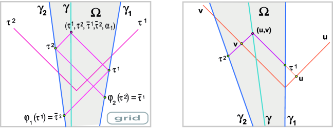
Figure 2: (a) Emitter positioning data $\{\tau^{1},\tau^{2};\bar{\tau}^{1},\bar{\tau}^{2}\}$ allowing the user $\gamma$ to find that, in the grid, (i) the trajectories of the two emitters $\gamma_{1}$, $\gamma_{2}$ are two straight lines with complementary slope, (ii) his own trajectory is a straight line parallel to the bisector. (b) If the user also receives an identically vanishing acceleration of an emitter, say $\alpha_{1}=0$, he obtains that he and the emitters have an inertial motion, and that his relative velocity with respect to every emitter is the same. Here we have drawn the trajectories in an inertial system at rest with respect to $\gamma_{1}$.

IV Information provided by the user data: the case of inertial emitters

The positioning system defined in Minkowski plane by two inertial emitters has been analyzed in a previous paper cfm-a . There we started from the proper time history of the emitters in an inertial null coordinate system and we studied what would be the data that a user of the positioning system would receive. Here we want to use this positioning system to illustrate the results presented in the above section. Thus, now we will start, on one hand, from the data received by an arbitrary user to obtain information on the (positioning) system following the steps of subsection III.4 and, on the other hand, from the data received by a specific user to obtain information about himself following the steps of subsection III.5.

IV.1 System information

Assumption S: The data $I\equiv\{\tau^{1},\tau^{2};\bar{\tau}^{1},\bar{\tau}^{2},\alpha_{1}\}$ received by any user in the emission coordinate domain is such that:

-

the pairs of data $\{\tau^{1};\bar{\tau}^{2}\}$ and $\{\tau^{2};\bar{\tau}^{1}\}$ show a linear relation with the same slope,

$$\hskip 8.53581pt\bar{\tau}^{1}=\displaystyle\tau^{2}_{0}+\lambda\,\tau^{1}\,,\quad\bar{\tau}^{2}=\displaystyle\tau^{1}_{0}+\lambda\,\tau^{2}\,,$$

i.e., complementary slope in the grid $\{\tau^{1},\tau^{2}\}$ (see Fig. 2(a)),

-

the acceleration $\alpha_{1}$ identically vanishes, $\alpha_{1}=0,\ \forall\,\tau^{1}$.

Step s1: From the first item of this assumption S, any user obtains that the emitter trajectory functions $\varphi_{1}(\tau^{1})$ and $\varphi_{2}(\tau^{2})$ are, respectively:

$$\hskip 8.53581pt\varphi_{1}(\tau^{1})=\displaystyle\tau^{2}_{0}+\lambda\,\tau^{1}\,,\quad\varphi_{2}(\tau^{2})=\displaystyle\tau^{1}_{0}+\lambda\,\tau^{2}\,.$$ (21)

Step s2: From the second item, any user obtains that the emitter acceleration scalar $\alpha_{1}(\tau^{1})$ is:

$$\alpha_{1}(\tau^{1})=0\,.$$

Step s3: From the acceleration scalar $\alpha_{1}(\tau^{1})$ obtained in step s2 any user obtains that the shift $s_{1}(\tau^{1})$ with respect to any inertial system is constant. Let $\{\texttt{u},\texttt{v}\}$ be an inertial system such that:

$$s_{1}(\tau^{1})=1\,.$$

Step s4: From the function $\varphi_{2}(\tau^{2})$ obtained in step s1 and the shift $s_{1}(\tau^{1})$ obtained in step s3 any user obtains that the shift $s_{2}(\tau^{2})$ with respect to the inertial system $\{\texttt{u},\texttt{v}\}$, and the acceleration $\alpha_{2}(\tau^{2})$ are, respectively:

$$\qquad s_{2}(\tau^{2})=\lambda\,,\quad\alpha_{2}(\tau^{2})=0\,.$$

Step s5: From the shifts $s_{1}(\tau^{1})$ and $s_{2}(\tau^{2})$ obtained in steps s3 and s4 any user obtains that the metric function in emission coordinates is:

$$m(\tau^{1},\tau^{2})=\frac{1}{\lambda}\,.$$

Step s6: From the shifts $s_{1}(\tau^{1})$ and $s_{2}(\tau^{2})$ obtained in steps s3 and s4 any user obtains that the transformation from emission to the inertial null system $\{\texttt{u},\texttt{v}\}$ (for a choice of the origin) is:

$$\begin{array}[]{l}\displaystyle\texttt{u}=u_{1}(\tau^{1})=\tau^{1}\,,\\[4.2679pt] \displaystyle\texttt{v}=v_{2}(\tau^{2})=\frac{1}{\lambda}(\tau^{2}-\tau^{2}_{0})\,.\end{array}$$

Step s7: From the functions $\varphi_{1}(\tau^{1})$ and $\varphi_{2}(\tau^{2})$ obtained in step s1 and the coordinate transformation $\{u_{1}(\tau^{1}),v_{2}(\tau^{2})\}$ obtained in step s6 any user obtains that the proper time history of the emitters in the inertial null coordinates $\{\texttt{u},\texttt{v}\}$ are, respectively:

$$\quad\quad\gamma_{1}\equiv\begin{cases}\texttt{u}=\tau^{1}\\ \texttt{v}=\tau^{1}\,,\end{cases}\quad\gamma_{2}\equiv\begin{cases}\texttt{u}=\tau^{1}_{0}+\lambda\,\tau^{2}\\ \texttt{v}=\frac{1}{\lambda}(\tau^{2}-\tau^{2}_{0})\,.\end{cases}$$

Steps s2 and s4 show that a user can receive the assumed set of data $I$ only if the positioning system is defined by two inertial emitters. In step 3, the arbitrary constant factor has been chosen so that emitter $\gamma_{1}$ is at rest with respect the inertial system $\{\texttt{u},\texttt{v}\}$ (see Fig. 2(b)). Moreover, from step s6 we obtain that, in the orthonormal coordinate system $\{t,x\}$ associated with the null one $\{\texttt{u},\texttt{v}\}$, the proper time history of the emitter $\gamma_{1}$ is $\{t=\tau^{1};\ x=0\}$. This means that we have chosen the additive constants in step s6 so that the origin of the inertial system is at the event which the emitter $\gamma_{1}$ reaches when his proper time clock watches zero.

IV.2 User information

Now we will illustrate how a specific user, receiving the emitter positioning data and the acceleration of one of the emitters, can determine his time and his dynamics.

Assumption U: The specific user in question receives the user data $I\equiv\{\tau^{1},\tau^{2};\bar{\tau}^{1},\bar{\tau}^{2},\alpha_{1}\}$ of the above assumption S and, in addition:

-

the data $\{\tau^{1};\tau^{2}\}$ show a linear relation with slope $1$ (see Fig. 2(a)).

Step u1: From these data, and following steps s1, s2, s3, s4 and s6 above, the user has obtained the coordinate transformation $\{u_{1}(\tau^{1}),v_{2}(\tau^{2})\}$ from emission to inertial coordinates $\{\texttt{u},\texttt{v}\}$.

Step u2: From the above assumption U the user obtains that his trajectory in the grid is:

$$\tau^{2}=F(\tau^{1})=\tau^{1}+C\,.$$

Step u3: From this user trajectory $\tau^{2}=F(\tau^{1})$ obtained in step u2 and the coordinate transformation $\{u_{1}(\tau^{1}),v_{2}(\tau^{2})\}$ obtained in step u1 the user obtains that his world line $\texttt{v}=f(\texttt{u})$ in the inertial system $\{\texttt{u},\texttt{v}\}$ is:

$$\texttt{v}=f(\texttt{u})=\frac{1}{\lambda}(\texttt{u}+C-\tau_{0}^{2})\,.$$

Step u4: From the user world line $\texttt{v}=f(\texttt{u})$ obtained in step u3 the user can obtain that his proper time function $\tau={\cal T}(\texttt{u})$ is:

$$\tau={\cal T}(\texttt{u})=\frac{1}{\sqrt{\lambda}}\,\texttt{u}\,.$$

Step u5: From the user proper time function $\tau={\cal T}(\texttt{u})$ obtained in step u4 and the user world line $\texttt{v}=f(\texttt{u})$ obtained in step u3 the user obtains that his proper time history in the inertial null coordinates $\{\texttt{u},\texttt{v}\}$ is:

$$\quad\gamma\equiv\begin{cases}\texttt{u}=\texttt{u}(\tau)=\sqrt{\lambda}\,\tau\\ \displaystyle\texttt{v}=\texttt{v}(\tau)=\frac{1}{\sqrt{\lambda}}\,\tau+\frac{1}{\lambda}(C-\tau_{0}^{2})\,.\end{cases}$$

Step u6: From the proper time history of the user in the inertial null coordinates $\{\texttt{u}=\texttt{u}(\tau),\texttt{v}=\texttt{v}(\tau)\}$ obtained in step u5 the user obtains that his shift $s(\tau)$ with respect the inertial system $\{\texttt{u},\texttt{v}\}$, and his acceleration $\alpha(\tau)$:

$$s(\tau)=\sqrt{\lambda}\,,\qquad\quad\alpha(\tau)=0\,.$$

Step u7: From the proper time history of the user in the inertial null coordinates $\{\texttt{u}=\texttt{u}(\tau),\texttt{v}=\texttt{v}(\tau)\}$ obtained in step u5 and the coordinate transformation $\{u_{1}(\tau^{1}),v_{2}(\tau^{2})\}$ obtained in step u1 the user obtains that his proper time history in emission coordinates is:

$$\quad\quad\quad\gamma\equiv\begin{cases}\tau^{1}=\psi_{1}(\tau)=\sqrt{\lambda}\,\tau\,,\\[2.27621pt] \tau^{2}=\psi_{2}(\tau)=\sqrt{\lambda}\,\tau+C\,.\end{cases}$$

and the user proper time lapse $\Delta\tau$ is:

$$\Delta\tau=\frac{1}{\sqrt{\lambda}}\,\Delta\tau^{1}=\frac{1}{\sqrt{\lambda}}\,\Delta\tau^{2}\,.$$

Let us note that the hyperbolic angle between the trajectories of the user and the emitter $\gamma_{1}$ is $\phi=\ln s(\tau)=\frac{1}{2}\ln\lambda$, and the hyperbolic angle between the trajectories of the emitters $\gamma_{2}$ and $\gamma_{1}$ is $\phi_{2}=\ln s_{2}(\tau^{2})=\ln\lambda=2\phi$. Consequently, the user has the same relative velocity with respect to both emitters. (see Fig. 2(b)). On the other hand, in the proper time function obtained in step u4 we have chosen the additive constant so that the user proper time clock watches zero when time $\tau^{1}=0$ is received by the user.

V Information provided by the user data: the case of stationary emitters

The positioning system defined in Minkowski plane by two (stationary) uniformly accelerated emitters has been analyzed in a previous paper cfm-b . There we supposed that the user knew, a priory, that the system was stationary. Here we start from the emitter positioning data and the acceleration of an emitter and, following the steps presented in subsections III.4 and III.5, we obtain all the system and user information.

V.1 System information

Assumption S: The data $A\equiv\{\tau^{1},\tau^{2};\bar{\tau}^{1},\bar{\tau}^{2},\alpha_{1}\}$ received by any user in the emission coordinate domain is such that:

-

the pairs of data $\{\tau^{1};\bar{\tau}^{2}\}$ and $\{\tau^{2};\bar{\tau}^{1}\}$ show linear relations with inverse slopes,

$$\hskip 8.53581pt\bar{\tau}^{1}=\displaystyle\frac{1}{\omega}(\tau^{1}-q-\sigma)\,,\quad\bar{\tau}^{2}=\displaystyle\omega\tau^{2}-q+\sigma\,,$$

with $\omega>1$ and $q>0$, i.e., parallel straight lines in the grid $\{\tau^{1},\tau^{2}\}$ (see Fig. 3(a)),

-

the acceleration $\alpha_{1}$ takes the constant value $\alpha_{1}=\frac{1}{q}\ln\omega,\ \forall\,\tau^{1}$.

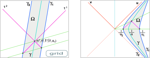
Figure 3: (a) Emitter positioning data $\{\tau^{1},\tau^{2};\bar{\tau}^{1},\bar{\tau}^{2}\}$ allowing the user $\gamma$ to find that, in the grid, (i) the trajectories of the two emitters $\gamma_{1}$, $\gamma_{2}$ are two parallel straight lines, (ii) his own trajectory is a straight line parallel to the emitters. Here we have plotted the case $c=0$ and we have stressed the user when receiving vanishing emitter coordinates. (b) If the user also receives the acceleration of the emitter $\gamma_{1}$ with the constant value $\alpha_{1}=\frac{1}{q}\ln\omega$, where $\omega$ is the slope parameter and $q$ is the separation parameter, he obtains that he and the emitters have a non inertial stationary motion, and he can determine their constant accelerations and their synchronization. Here we have drawn the trajectories when the synchronization parameter $\sigma=0$. In green we have drawn the locus of simultaneous events for the stationary congruence.

Step s1: From the first item of this assumption S, any user obtains that the emitter trajectory functions $\varphi_{1}(\tau^{1})$ and $\varphi_{2}(\tau^{2})$ are, respectively:

$$\begin{array}[]{l}\varphi_{1}(\tau^{1})=\displaystyle\frac{1}{\omega}(\tau^{1}-q-\sigma)\,,\\[8.53581pt] \varphi_{2}(\tau^{2})=\displaystyle\omega\tau^{2}-q+\sigma\,.\end{array}$$ (22)

Step s2: From the second item any user obtains that the emitter acceleration scalar $\alpha_{1}(\tau^{1})$ is:

$$\alpha_{1}(\tau^{1})=\frac{1}{q}\ln\omega\equiv\alpha_{1}\,.$$

Step s3: From the acceleration scalar $\alpha_{1}(\tau^{1})$ obtained in step s2 any user obtains that the shift $s_{1}(\tau^{1})$ with respect to an inertial system $\{\texttt{u},\texttt{v}\}$ (fixed up to a choice of the origin) is:

$$s_{1}(\tau^{1})=\exp(\alpha_{1}\tau^{1})\,.$$

Step s4: From the function $\varphi_{2}(\tau^{2})$ obtained in step s1 and the shift $s_{1}(\tau^{1})$ obtained in step s3 any user obtains that the shift $s_{2}(\tau^{2})$ with respect to the inertial system $\{\texttt{u},\texttt{v}\}$, and the acceleration $\alpha_{2}(\tau^{2})$ are:

$$\qquad s_{2}(\tau^{2})=\exp(\alpha_{2}(\tau^{2}-\tau^{2}_{0}))\,,\quad\alpha_{2}(\tau^{2})=\alpha_{2}\,,$$

where $\alpha_{2}\equiv\omega\alpha_{1}$, and $\tau^{2}_{0}\equiv-\frac{\sigma}{\omega}$.

Step s5: From the shifts $s_{1}(\tau^{1})$ and $s_{2}(\tau^{1})$ obtained in steps s3 and s4 any user obtains that the metric function in emission coordinates is:

$$m(\tau^{1},\tau^{2})=\omega^{\frac{1}{q}(\tau^{1}-\omega\tau^{2}-\sigma)}\,.$$

Step s6: From the shifts $s_{1}(\tau^{1})$ and $s_{2}(\tau^{2})$ obtained in steps s3 and s4 any user obtains that the transformation from emission to the inertial null system $\{\texttt{u},\texttt{v}\}$ (for a choice of the origin) is:

$$\begin{array}[]{l}\displaystyle\texttt{u}=u_{1}(\tau^{1})=\frac{1}{\alpha_{1}}\,\exp(\alpha_{1}\tau^{1})\,,\\[8.53581pt] \displaystyle\texttt{v}=v_{2}(\tau^{2})=-\frac{1}{\alpha_{2}}\,\exp(-\alpha_{2}(\tau^{2}-\tau^{2}_{0}))\,.\end{array}$$

Step s7: From the functions $\varphi_{1}(\tau^{1})$ and $\varphi_{2}(\tau^{2})$ obtained in step s1 and the coordinate transformation $\{u_{1}(\tau^{1}),v_{2}(\tau^{2})\}$ obtained in step s6 any user obtains that the proper time history of the emitters in inertial null coordinates $\{\texttt{u},\texttt{v}\}$ is:

$$\begin{array}[]{l}\quad\gamma_{1}\!\equiv\!\begin{cases}\displaystyle\texttt{u}=\frac{1}{\alpha_{1}}\,\exp(\alpha_{1}\tau^{1})\\ \displaystyle\texttt{v}=-\frac{1}{\alpha_{1}}\,\exp(-\alpha_{1}\tau^{1})\,,\end{cases}\\[19.91692pt] \quad\gamma_{2}\!\equiv\!\begin{cases}\displaystyle\texttt{u}=\frac{1}{\alpha_{2}}\,\exp(\alpha_{2}(\tau^{2}-\tau^{2}_{0}))\\ \displaystyle\texttt{v}=-\frac{1}{\alpha_{2}}\,\exp(-\alpha_{2}(\tau^{2}-\tau^{2}_{0}))\,.\end{cases}\end{array}$$

Steps s2 and s4 show that a user receiving the set of data $A$ is, necessarily, in the coordinate domain of a positioning system defined by two uniformly accelerated emitters with constant acceleration scalars $\alpha_{1}(\tau_{1})=\frac{1}{q}\ln\omega\equiv\alpha_{1}$ and $\alpha_{2}(\tau_{2})=\omega\alpha_{1}>\alpha_{1}$. In step s3, the arbitrary constant factor has been chosen so that emitter $\gamma_{1}$ is at rest with respect the inertial system $\{\texttt{u},\texttt{v}\}$ when his proper time clock watches zero.

From step s7, we have that the emitter trajectories in the inertial system are $\alpha_{i}^{2}\texttt{u}\texttt{v}=-1$. This means that in step s6 we could choose the additive constants (i.e., the origin of the inertial coordinate system) so that the coordinate bisectors are the asymptotes of both emitter trajectories (see Fig. 3(b)). Thus, the emitters maintain a constant radar distance and, consequently, they belong to a congruence of stationary observers. On the other hand, $\tau^{2}_{0}\equiv-\frac{\sigma}{\omega}$ gives the time which watches the proper time clock of $\gamma_{2}$ at the event simultaneous to the event where the proper time clock of $\gamma_{1}$ watches zero. This fact shows that in relativistic positioning the synchronization between the emitter clocks is not necessary, but it can be extracted from the emitter data.

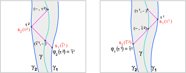
Figure 4: Geometric interpretation of the constraint equations: (a) If a user receives the trajectory $\bar{\tau}^{1}=\varphi_{2}(\tau^{2})$ in the vicinity of time $\tau^{2}$ and the shift $s_{1}(\bar{\tau}^{1})$ at time $\bar{\tau}^{1}$, then he can obtain the shift $s_{2}(\tau^{2})$ at time $\tau^{2}$. (b) If a user receives the trajectory $\bar{\tau}^{2}=\varphi_{1}(\tau^{1})$ in the vicinity of time $\tau^{1}$ and the shift $s_{2}(\bar{\tau}^{2})$ at time $\bar{\tau}^{2}$, then he can obtain the shift $s_{1}(\tau^{1})$ at time $\tau^{1}$.

V.2 User information

Now we will illustrate how a specific user, receiving the emitter positioning data and the acceleration of one of the emitters, can determine his time and his dynamics.

Assumption U: The specific user in question receives the user data $A\equiv\{\tau^{1},\tau^{2};\bar{\tau}^{1},\bar{\tau}^{2},\alpha_{1}\}$ of the above assumption S and, in addition:

-

the data $\{\tau^{1};\tau^{2}\}$ show a linear relation with the same slope than the emitters (parallel to the emitter trajectories in the grid $\{\tau^{1},\tau^{2}\}$; see Fig. 3(a)).

Step u1: From these data, and following steps s1, s2, s3, s4 and s6 above, the user has obtained the coordinate transformation $\{u_{1}(\tau^{1}),v_{2}(\tau^{2})\}$ from emission to inertial coordinates $\{\texttt{u},\texttt{v}\}$.

Step u2: From the above assumption U the user can obtain that his trajectory in the grid is:

$$\qquad\tau^{2}=F(\tau^{1})=\frac{1}{\omega}(\tau^{1}-c)\,,\quad q<c-\sigma<q\,.$$

Step u3: From the user trajectory $\tau^{2}=F(\tau^{1})$ obtained in step u2 and the coordinate transformation $\{u_{1}(\tau^{1}),v_{2}(\tau^{2})\}$ obtained in step u1 the user obtains that his world line $\texttt{v}=f(\texttt{u})$ in the inertial system $\{\texttt{u},\texttt{v}\}$ is:

$$\qquad\begin{array}[]{l}\displaystyle\texttt{v}=f(\texttt{u})=-\frac{1}{\alpha^{2}\texttt{u}}\,,\qquad\texttt{u}\,\texttt{v}=-\frac{1}{\alpha^{2}}\,,\\[8.53581pt] \displaystyle\alpha\equiv\frac{\ln\omega}{q}\omega^{\frac{1}{2q}(q+\sigma-c)}=\alpha_{1}^{\frac{1}{2q}(q-\sigma+c)}\alpha_{2}^{\frac{1}{2q}(q+\sigma-c)}\,.\end{array}$$

Step u4: From the user world line $\texttt{v}=f(\texttt{u})$ obtained in step u3 the user obtains that his proper time function $\tau={\cal T}(\texttt{u})$ is:

$$\tau={\cal T}(\texttt{u})=\frac{1}{\alpha}\,\ln(\alpha\texttt{u})\,.$$

Step u5: From the user proper time function $\tau={\cal T}((\texttt{u})$ obtained in step u4 and the user world line $\texttt{v}=f(\texttt{u})$ obtained in step u3 the user obtains that his proper time history in the inertial null coordinates $\{\texttt{u},\texttt{v}\}$ is:

$$\quad\gamma\equiv\begin{cases}\displaystyle\texttt{u}=\texttt{u}(\tau)=\frac{1}{\alpha}\,\exp(\alpha\tau)\\ \displaystyle\texttt{v}=\texttt{v}(\tau)=-\frac{1}{\alpha}\,\exp(-\alpha\tau)\,.\end{cases}$$

Step u6: From the proper time history of the user in the inertial null coordinates $\{\texttt{u}=\texttt{u}(\tau),\texttt{v}=\texttt{v}(\tau)\}$ obtained in step u5 the user obtains that his shift $s(\tau)$ with respect the inertial system $\{\texttt{u},\texttt{v}\}$, and his acceleration $\alpha(\tau)$ are, respectively:

$$s(\tau)=\exp(\alpha\tau)\,,\qquad\quad\alpha(\tau)=\alpha\,.$$

Step u7: From the proper time history of the user in the inertial null coordinates $\{\texttt{u}=\texttt{u}(\tau),\texttt{v}=\texttt{v}(\tau)\}$ obtained in step u5 and the coordinate transformation $\{u_{1}(\tau^{1}),v_{2}(\tau^{2})\}$ obtained in step u1 the user obtains that his proper time history in emission coordinates is:

$$\quad\quad\gamma\equiv\begin{cases}\displaystyle\tau^{1}=\frac{\alpha}{\alpha_{1}}\,\tau-\frac{1}{2}(q+\sigma-c)\,,\\[5.69054pt] \displaystyle\tau^{2}=\frac{\alpha}{\alpha_{2}}\,\tau-\frac{1}{2\omega}(q+\sigma+c)\,.\end{cases}$$

and his proper time lapse $\Delta\tau$ is:

$$\Delta\tau=\frac{\alpha_{1}}{\alpha}\,\Delta\tau^{1}=\frac{\alpha_{2}}{\alpha}\,\Delta\tau^{2}\,,$$

where $\frac{\alpha}{\alpha_{1}}\equiv\omega^{\frac{1}{2q}(q+\sigma-c)}$ and $\frac{\alpha}{\alpha_{2}}\equiv\omega^{-\frac{1}{2q}(q-\sigma+c)}$.

Step u3 shows that the user also follows a stationary motion that keep a constant radar distance with respect the two emitters (see Fig. 3(b)). Moreover, the constant value of the acceleration of the user is the weighted geometric mean of the emitters’ accelerations. In the proper time function obtained in step u4 we have chosen the additive constant so that the events, where the proper time clocks of the user and of the emitter $\gamma_{1}$ watch zero, are simultaneous.

VI The delay master equation

In Sec. III we have shown that, as a consequence of the public data constraint equations (17) and (18), the emitter positioning data an the acceleration of an emitter determine the acceleration of the other emitter. Nevertheless, in the steps given in subsections III.4 and III.5, which allow to obtain all the system and user information, we only used one of these two restrictions or, more precisely only one of the two constraint equations for the shift (15) and (16). Do these equations impose stronger restrictions on the public data?

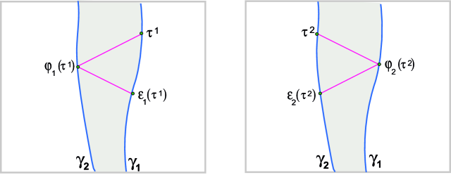
Figure 5: Geometric interpretation of the past echo functions $\varepsilon_{i}$ and the echo intervals $[\varepsilon_{1}(\tau^{1}),\tau^{1}]$ and $[\varepsilon_{2}(\tau^{2}),\tau^{2}]$: (a) If $\gamma_{1}$ receives at time $\tau^{1}$ a signal after being echoed by $\gamma_{2}$, it must be emitted at time $\varepsilon_{1}(\tau^{1})$. (b) If $\gamma_{2}$ receives at time $\tau^{2}$ a signal after being echoed by $\gamma_{1}$, it must be emitted at time $\varepsilon_{2}(\tau^{2})$.

In this section we will see that the answer is affirmative by obtaining the precise restrictions that the emitter positioning data impose on the dynamics of the emitters. This study requires to consider the shift constraint equations (15) and (16), not as two independent equations, but as a constraint system:

$$s_{2}(\tau^{2})=\dot{\varphi}_{2}(\tau^{2})\,s_{1}(\varphi_{2}(\tau^{2}))\,,$$ (23)

$$s_{1}(\tau^{1})\,\dot{\varphi}_{1}(\tau^{1})=s_{2}(\varphi_{1}(\tau^{1}))\,.$$ (24)

VI.1 The (past) echo functions and the delay master equation

In Secs. III, IV and V, when we obtained an emitter acceleration from the emitter positioning data and the acceleration of the other emitter, we supposed that the user received continuously these data. Now, in order to better understand the constraints on the public data, it is useful to analyze its local behavior. In this sense, the constraint system (23)-(24) can be read as follows (see Fig. 4):
Statement 7.– (i) If a user receives the trajectory $\bar{\tau}^{1}=\varphi_{2}(\tau^{2})$ in the vicinity of time $\tau^{2}$ and the shift $s_{1}(\bar{\tau}^{1})$ at time $\bar{\tau}^{1}$, then he can obtain the shift $s_{2}(\tau^{2})$ at time $\tau^{2}$.

(ii) If a user receives the trajectory $\bar{\tau}^{2}=\varphi_{1}(\tau^{1})$ in the vicinity of time $\tau^{1}$ and the shift $s_{2}(\bar{\tau}^{2})$ at time $\bar{\tau}^{2}$, then he can obtain the shift $s_{1}(\tau^{1})$ at time $\tau^{1}$.

This interpretation of the constraint system has important consequences. Let us define the past echo functions $\varepsilon_{i}$ as follows:

$$\varepsilon_{1}=\varphi_{2}\circ\varphi_{1}\,,\qquad\varepsilon_{2}=\varphi_{1}\circ\varphi_{2}\,.$$ (25)

These (past) echo functions have the following geometric interpretation (see Fig. 5):

• If $\gamma_{1}$ receives at time $\tau^{1}$ a signal after being echoed by $\gamma_{2}$, it must be emitted at time $\varepsilon_{1}(\tau^{1})$.

• If $\gamma_{2}$ receives at time $\tau^{2}$ a signal after being echoed by $\gamma_{1}$, it must be emitted at time $\varepsilon_{2}(\tau^{2})$.

The proper time intervals $[\varepsilon_{1}(\tau^{1}),\tau^{1}]$ and $[\varepsilon_{2}(\tau^{2}),\tau^{2}]$ are named (causal) echo intervals, i.e., an echo interval is the interval between the emission of a signal by an emitter and its reception after being reflected by the other emitter (see Fig. 5).

Let us suppose that a user receives the emitter acceleration $\alpha_{1}$ (and so he knows the shift $s_{1}$) in the echo interval $[\varepsilon_{1}(\tau^{1}),\tau^{1}]$, and that he also receives the emitter positioning data $\{\tau^{1},\tau^{2};\bar{\tau}^{1},\bar{\tau}^{2}\}$ along the arc $[\varphi_{1}(\tau^{1}),\varphi_{2}^{-1}(\tau^{1})]$ that is, he knows the emitter trajectories $\varphi_{i}(\tau^{i})$ along this arc. Then the user knows the shift $s_{2}$ along the arc $[\varphi_{1}(\tau^{1}),\varphi_{2}^{-1}(\tau^{1})]$ as a consequence of (23) (see Fig. 6(a)). Therefore the user knows the shift $s_{1}$ in the echo interval $[\tau^{1},\varepsilon_{1}^{-1}(\tau^{1})]$ as a consequence of (24). And so on (see Fig. 6(b)).

We can obtain the analytical expression of this fact by replacing $\tau^{2}$ by $\varphi_{1}(\tau^{1})$ in equation (23) and substituting in (24). Then we arrive to the delay master equation:

$$s_{1}(\tau^{1})=\frac{\dot{\varphi}_{2}(\varphi_{1}(\tau^{1}))}{\dot{\varphi}_{1}(\tau^{1})}s_{1}(\varepsilon_{1}(\tau^{1}))\,.$$ (26)

In a similar way, by replacing $\tau^{1}$ with $\varphi_{2}(\tau^{2})$ in equation (24) and substituting in (23), we obtain:

$$s_{2}(\tau^{2})=\frac{\dot{\varphi}_{2}(\tau^{2})}{\dot{\varphi}_{1}(\varphi_{2}(\tau^{2}))}s_{2}(\varepsilon_{2}(\tau^{2}))\,.$$ (27)

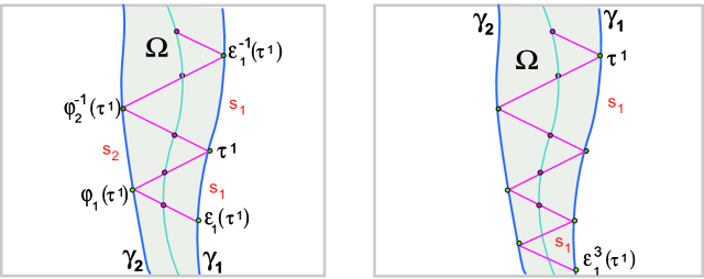
Figure 6: Geometric interpretation of the master delay equation: (a) If a user receives the emitter positioning data $\{\tau^{1},\tau^{2};\bar{\tau}^{1},\bar{\tau}^{2}\}$ along the arc $[\varphi_{1}(\tau^{1}),\varphi_{2}^{-1}(\tau^{1})]$ and the emitter shift $s_{1}$ in the echo interval $[\varepsilon_{1}(\tau^{1}),\tau^{1}]$, then the user knows the shift $s_{2}$ in the arc $[\varphi_{1}(\tau^{1}),\varphi_{2}^{-1}(\tau^{1})]$ as a consequence of (23). Therefore the user knows the shift $s_{1}$ in the echo interval $[\tau^{1},\varepsilon_{1}^{-1}(\tau^{1})]$ as a consequence of (24). (b) The delay master equations can be applied repeatedly in order to obtain an emitter shift further from an echo interval.

The delay master equations (26) and (27) can be written in terms of the echo operators $Q_{i}(\tau^{i})$ as:

$$s_{1}(\tau^{1})=Q_{1}(\tau^{1})s_{1}(\varepsilon_{1}(\tau^{1})),\ \ Q_{1}(\tau^{1})\equiv\frac{\dot{\varphi}_{2}(\varphi_{1}(\tau^{1}))}{\dot{\varphi}_{1}(\tau^{1})},\quad$$ (28)

$$s_{2}(\tau^{2})=\frac{1}{Q_{2}(\tau^{2})}s_{2}(\varepsilon_{2}(\tau^{2})),\ \ Q_{2}(\tau^{2})\equiv\frac{\dot{\varphi}_{1}(\varphi_{2}(\tau^{2}))}{\dot{\varphi}_{2}(\tau^{2})}.\quad$$ (29)

Evidently, we can obtain the emitter shifts further from an echo interval by applying the delay master equation repeatedly. This fact can be expressed by using the n-echo operators $Q_{i}^{n}(\tau^{i})$ (see Fig. 6(b)):

$$s_{1}(\tau^{1})=Q_{1}^{n}(\tau^{1})s_{1}(\varepsilon_{1}^{n}(\tau^{1}))\,,$$ (30)

$$s_{2}(\tau^{2})=\frac{1}{Q_{2}^{n}(\tau^{2})}s_{2}(\varepsilon_{2}^{n}(\tau^{2}))\,,$$ (31)

$$Q_{i}^{n}(\tau^{i})\!\equiv\!\prod_{r=0}^{n-1}Q_{i}(\varepsilon_{i}^{r}(\tau^{i}))\,.$$ (32)

These equations allow to state:
Statement 8.– A user may know the shift of an emitter along his trajectory provided that he receives the shift during a sole echo interval and the emitter positioning data along his trajectory.

VI.2 Getting the dynamics by means of the delay master equation

Now, we can use the delay master equation to improve the results in Sec. III. Indeed, if we take into account these results and statement 8, we arrive to:
Statement 9.– If a user receives the emitter positioning data $\{\tau^{1},\tau^{2};\bar{\tau}^{1},\bar{\tau}^{2}\}$ along his trajectory and the acceleration of one of the emitters during a sole echo interval, then this user can obtain a full information about his dynamics and the dynamics of the emitters.

In order to obtain all this information in a specific situation it is worth analyzing what is the minimum set of equations which are necessary. We have obtained the master delay equations (26) and (27) from the constraint system (23)-(24), and a straightforward calculation allows to show:
Statement 10.- If the emitter trajectories in the grid $\varphi_{1}(\tau^{1})$ and $\varphi_{2}(\tau^{2})$ are known, then one of the constraint equations (23)-(24) and one of the master delay equations (26)-(27) imply the full constraint system (23)-(24).

Then, we can slightly modify the steps given in subsections III.4 and III.5 in order to obtain all the system and user information from a minimal set of public data.

Received user data: the emitter positioning data $\{\tau^{1},\tau^{2};\bar{\tau}^{1},\bar{\tau}^{2}\}$ along the user trajectory and the acceleration of an emitter, say $\alpha_{1}$, in an echo interval.

Step s1: From the pairs $\{\tau^{1};\bar{\tau}^{2}\}$ and $\{\tau^{2};\bar{\tau}^{1}\}$, determine the emitter trajectory functions $\varphi_{1}(\tau^{1})$ and $\varphi_{2}(\tau^{2})$, respectively.

Step s2^′: From the pair $\{\tau^{1};\alpha_{1}\}$, determine the emitter acceleration scalar $\alpha_{1}(\tau^{1})$ in the echo interval.

Step s3^′: From the acceleration scalar $\alpha_{1}(\tau^{1})$ obtained in step s2^′, determine the shift $s_{1}(\tau^{1})$ with respect to an inertial system $\{\texttt{u},\texttt{v}\}$ in the echo interval.

Step s3^′′: From the shift $s_{1}(\tau^{1})$ in the echo interval obtained in step s3^′, determine the shift $s_{1}(\tau^{1})$ with respect to an inertial system $\{\texttt{u},\texttt{v}\}$ along the user trajectory:

$$\qquad s_{1}(\tau^{1})=\frac{\dot{\varphi}_{2}(\varphi_{1}(\tau^{1}))}{\dot{\varphi}_{1}(\tau^{1})}s_{1}(\varepsilon_{1}(\tau^{1}))\,,\quad\varepsilon_{1}=\varphi_{2}\circ\varphi_{1}\,.$$

Steps s4-s7: From the function $\varphi_{2}(\tau^{2})$ obtained in step s1 and the shift $s_{1}(\tau^{1})$ obtained in step s3^′′, determine: the shift $s_{2}(\tau^{2})$ with respect to the inertial system $\{\texttt{u},\texttt{v}\}$ and the acceleration scalar $\alpha_{2}(\tau^{2})$, the metric function in emission coordinates, the transformation from emission to inertial null coordinates $\{\texttt{u},\texttt{v}\}$, and the proper time history of the emitters in these inertial coordinates along the whole emitter world lines.

Steps u1-u7: From the steps s1, s2, s3^′′, s4 and s6 and the pair $\{\tau^{1};\tau^{2}\}$, determine: the user trajectory in the grid, the user world line in the inertial system $\{\texttt{u},\texttt{v}\}$, the user proper time function $\tau={\cal T}(\texttt{u})$, the proper time history of the user in the inertial null coordinates $\{\texttt{u},\texttt{v}\}$, the shift $s(\tau)$ of the user with respect the inertial system $\{\texttt{u},\texttt{v}\}$ and the user acceleration $\alpha(\tau)$, and the proper time history of the user in emission coordinates.

VI.3 The delay master equation in positioning with inertial emitters

Let us suppose that the user receives along his trajectory a set of emitter positioning data $\{\tau^{1},\tau^{2};\bar{\tau}^{1},\bar{\tau}^{2}\}$ that leads, following step s1, to the emitter trajectories (21) in the grid. Thus, the echo function $\varepsilon_{1}$ and the echo operator $Q_{1}$ are, respectively,

$$\varepsilon_{1}(\tau^{1})=\lambda^{2}\tau^{1}+p\,,\qquad Q_{1}(\tau^{1})=1\,,$$ (33)

where $p\equiv\lambda\tau_{0}^{2}+\tau_{0}^{1}$. Then, the delay master equation for the shift $s_{1}(\tau^{1})$ takes the expression:

$$s_{1}(\tau^{1})=s_{1}(\lambda\tau^{1}+p)\,.$$ (34)

Let us suppose moreover that, following step s2^′, the data $\{\tau^{1};\alpha_{1}\}$ determine that the acceleration scalar identically vanishes in an echo interval, $\alpha_{1}(\tau^{1})=0$. Then, following step s3^′, a null inertial system $\{\texttt{u},\texttt{v}\}$ exists such that the shift in this echo interval is $s_{1}(\tau^{1})=1$. Now, in step s3^′′, we apply the delay master equation (34) and obtain $s_{1}(\tau^{1})=1$ along the user trajectory. At this point, following the steps s4-s7 and u1-u7 we obtain all the system and user information as we did in Sec. IV.

VI.4 The delay master equation in positioning with stationary emitters

Let us suppose that the user receives along his trajectory a set of emitter positioning data $\{\tau^{1},\tau^{2};\bar{\tau}^{1},\bar{\tau}^{2}\}$ that leads, following step s1, to the emitter trajectories (22) in the grid. Thus, the echo function $\varepsilon_{1}$ and the echo operator $Q_{1}$ are, respectively,

$$\varepsilon_{1}(\tau^{1})=\tau^{1}-2q\,,\qquad Q_{1}(\tau^{1})=\omega^{2}\,.$$ (35)

Then, the delay master equation for the shift $s_{1}(\tau^{1})$ takes the expression:

$$s_{1}(\tau^{1})=\omega^{2}s_{1}(\tau^{1}-2q)\,.$$ (36)

Let us suppose moreover that, following step s2^′, the data $\{\tau^{1};\alpha_{1}\}$ determine that the acceleration scalar takes the constant value $\alpha_{1}(\tau^{1})=\frac{1}{q}\ln\omega$ in an echo interval. Then, following step s3^′, a null inertial system $\{\texttt{u},\texttt{v}\}$ exists such that the shift in this echo interval is $s_{1}(\tau^{1})=\exp(\alpha_{1}\tau^{1})$. Now, in step s3^′′ we apply the master delay equation (36) and obtain $s_{1}(\tau^{1})=\exp(\alpha_{1}\tau^{1})$ along the user trajectory. At this point, following the steps s4-s7 and u1-u7 we obtain all the system and user information as we did in Sec. V.

VI.5 The delay equations for the emitter accelerations

In statement 7 we can replace the shifts $s_{1}$ and $s_{2}$ with the accelerations $\alpha_{1}$ and $\alpha_{2}$ as a consequence of the public data constraint equations (17) and (18). Then, from these equations or from the delay master equations (28)-(29), we can obtain the delay equations for the emitter acceleration scalars:

$$\alpha_{1}(\tau^{1})=\frac{\dot{Q}_{1}(\tau^{1})}{Q_{1}(\tau^{1})}+\alpha_{1}(\varepsilon_{1}(\tau^{1}))\dot{\varepsilon}_{1}(\tau^{1})\,,$$ (37)

$$\alpha_{2}(\tau^{2})=-\frac{\dot{Q}_{2}(\tau^{2})}{Q_{2}(\tau^{2})}+\alpha_{2}(\varepsilon_{2}(\tau^{2}))\dot{\varepsilon}_{2}(\tau^{2})\,.$$ (38)

Moreover, we can also obtain a restriction on the emitter accelerations further from an echo interval:

$$\alpha_{1}(\tau^{1})=\frac{\dot{Q}_{1}^{n}(\tau^{1})}{Q_{1}^{n}(\tau^{1})}+\alpha_{1}(\varepsilon_{1}(\tau^{1}))\dot{\varepsilon}_{1}^{n}(\tau^{1})\,,$$ (39)

$$\alpha_{2}(\tau^{2})=-\frac{\dot{Q}_{2}^{n}(\tau^{2})}{Q_{2}^{n}(\tau^{2})}+\alpha_{2}(\varepsilon_{2}(\tau^{2}))\dot{\varepsilon}_{2}^{n}(\tau^{2})\,.$$ (40)

Thus, as a consequence of these equations we can replace in statement 8 the emitter shift with the emitter acceleration.

The delay equations (37)-(38) for the emitter accelerations follow from the master equations (28)-(29) but they are not sufficient conditions.

Thus, if we know the acceleration of an emitter in an echo interval we must: firstly, obtain the shift and, secondly, apply the master equation, as explained in steps presented in section VI.2. If, on the contrary, we first apply the delay equation for the acceleration and, secondly, we determine the shift, we could lost a part of the information that the master equation provides.

We can better understand this point with an example. Let us suppose that the user receives along his trajectory a set of emitter positioning data that leads to the emitter trajectories (22) in the grid. And let us also suppose that he receives the acceleration of the emitter $\gamma_{1}$ in an echo interval with a constant value $\alpha_{1}$. Then, we can obtain the shift in this echo interval and the master equation (which takes the expression (36)) implies that, under a continuity assumption for the shifts, the accelerations takes, necessarily, the constant value $\alpha_{1}(\tau^{1})=\frac{1}{q}\ln\omega$.

Nevertheless, if we apply first the delay equation for the accelerations, $\alpha_{1}(\tau^{1})=\alpha_{1}(\tau^{1}-2q)$, we obtain $\alpha_{1}(\tau^{1})=\alpha_{1}$ independently of the value of $\alpha_{1}$. This apparent no constraint on $\alpha_{1}$ is deceptive: if we apply the steps s1-s7 presented in section III.4 for a value of the acceleration $\alpha_{1}\not=\frac{1}{q}\ln\omega$, we arrive to an inconsistency.

VII Discussion and work in progress

In this work we have analyzed the constraints on the data received by a user of a relativistic positioning system, and how these data can afford information on the dynamics of the user and of the emitters. We have shown that the user can obtain his acceleration and the acceleration of the emitters provided that he receives the emitter positioning data along his trajectory and the acceleration of only one of the emitters and only during a (causal) echo interval.

We have presented a protocol organized in steps which allows to obtain, from the minimal set of data, all the system and user information, namely, the acceleration of the emitters and of the user, the transformation from the emission to inertial null coordinates, and the proper time history of the emitters and of the user in this inertial system.

Our study shows that the delay master equation plays an essential role in the internal behavior of a positioning system built in a flat two-dimensional space-time. A forthcoming work should deal with looking for a similar constraint in a four-dimensional space-time and in presence of a gravitational field.

In a future extension to the four-dimensional case of the two-dimensional methods used here we should take into account the role that the angle between pairs of arrival signals could play in obtaining information on the metric tensor and on the positioning system.

Appendix A Two-dimensional kinematics in null coordinates

In a null coordinate system $\{\tau^{1},\tau^{2}\}$ the space-time metric depends on a sole metric function $m$:

$$ds^{2}=m(\tau^{1},\tau^{2})d\tau^{1}d\tau^{2}\,.$$ (41)

The proper time history of an observer $\gamma$ is:

$$\tau^{1}=\psi_{1}(\tau),\qquad\tau^{2}=\psi_{2}(\tau)\,,$$ (42)

and its tangent vector is:

$$T(\tau)=(\dot{\psi_{1}}(\tau),\dot{\psi_{2}}(\tau))\,,$$

where a dot means derivative with respect proper time. The unit condition for $T$ becomes:

$$m(\psi_{1}(\tau),\psi_{2}(\tau))=\frac{1}{\dot{\psi_{1}}(\tau)\dot{\psi_{2}}(\tau)}\,.$$ (43)

This relation implies that when the unit tangent vector of an observer is known in terms of his proper time, the metric on the trajectory of this observer is also known.

The proper time parameterized trajectory (42) is tantamount to a (geometric) trajectory $\tau^{2}=F(\tau^{1})$ and a proper time function $\tau=\tau(\tau^{1})$ related and restricted by the unit condition. Indeed, from one of the expressions (42) we can obtain the proper time of the observer $\gamma$, say:

$$\tau=\tau(\tau^{1})=\psi_{1}^{-1}(\tau^{1})\,.$$

Then, the trajectory is given by:

$$\tau^{2}=F(\tau^{1})=\psi_{2}(\psi_{1}^{-1}(\tau^{1}))\,,$$

and, in terms of $\tau^{2}=F(\tau^{1})$ and $\tau=\tau(\tau^{1})$, the unit condition (43) becomes:

$$[\tau^{\prime}(\tau^{1})]^{2}=m(\tau^{1},F(\tau^{1}))F^{\prime}(\tau^{1})\,.$$ (44)

From equation (44) it follows: if the the metric function is known, (i) there always exists a congruence of users having a prescribed proper time function, and (ii) the geometric trajectory of a observer determines his local unit of time.

The acceleration of the observer (42) in null coordinates $\{\tau^{1},\tau^{2}\}$ takes the expression:

$$a(\tau)=\left(\ddot{\psi_{1}}+(\ln m),_{1}\dot{\psi}_{1}^{2}\,,\;\ddot{\psi_{2}}+(\ln m),_{2}\dot{\psi}_{2}^{2}\right)\,,$$ (45)

and the acceleration scalar $\alpha(\tau)\equiv\pm\sqrt{-a^{2}(\tau)}$ is:

$$\alpha(\tau)=\frac{\ddot{\psi_{1}}}{\dot{\psi}_{1}}+(\ln m),_{1}\dot{\psi}_{1}=-\frac{\ddot{\psi_{2}}}{\dot{\psi}_{2}}-(\ln m),_{2}\dot{\psi}_{2}\,.$$ (46)

The dynamic equation, i.e. the equation for the world lines with a known acceleration $\alpha$, and consequently the geodesic equation (when $\alpha=0$), can be written as two coupled equations for the proper time functions $\psi_{1}(\tau)$ and $\psi_{2}(\tau)$:

$$\frac{\ddot{\psi_{1}}}{\dot{\psi}_{1}}+(\ln m),_{1}\dot{\psi}_{1}=\alpha(\tau)\,,\qquad m\dot{\psi}_{1}\dot{\psi}_{2}=1$$ (47)

In (47) the metric function $m(\tau^{1},\tau^{2})$ is known, and $m$ stands for $m(\tau^{1}(\tau),\tau^{2}(\tau))$; therefore, it is a coupled system.

Dynamic equation in flat metric

In a two-dimensional flat space-time the metric function $m$ in null coordinates $\{\tau^{1},\tau^{2}\}$ factorizes:

$$m(\tau^{1},\tau^{2})=u^{\prime}(\tau^{1})v^{\prime}(\tau^{2})\,,$$

where $\texttt{u}=u(\tau^{1})$ and $\texttt{v}=v(\tau^{2})$ give the transformation to an inertial coordinate system $\{\texttt{u},\texttt{v}\}$.

As a consequence of this factorization, the dynamic equation (47) can be partially integrate and it becomes:

$$\dot{\psi}_{1}(\tau)u^{\prime}(\psi_{1}(\tau))=\frac{1}{\dot{\psi}_{2}(\tau)v^{\prime}(\psi_{2}(\tau))}=s(\tau)\,,$$ (48)

where the shift parameter $s(\tau)$ is defined as:

$$s(\tau)\equiv\exp\left(\int\alpha(\tau)d\tau\right)\,.$$ (49)

Note that $s(\tau)$ is, actually, a shift parameter since it could be obtained as:

$$s(\tau)=\sqrt{\frac{1+\beta(\tau)}{1-\beta(\tau)}}$$ (50)

where $\beta(\tau)$ is the relative velocity between the given observer and an inertial one. The hyperbolic angle between both observers is $\,\phi(\tau)=\ln s(\tau)$.

References

- (1) B. Coll, in Proceedings Journées Systèmes de Référence, Bucarest, 2002, edited by N. Capitaine and M. Stavinschi (Observatoire de Paris, Paris, France, 2003). See also gr-qc/0306043.
- (2) B. Coll, J. J. Ferrando, and J. A. Morales, Phys. Rev. D 73, 084017 (2006).
- (3) B. Coll, J. J. Ferrando, and J. A. Morales, Phys. Rev. D 74, 104003 (2006).
- (4) B. Coll and J. M. Pozo, Class. Quantum Grav. 23, 7395 (2006).
- (5) B. Coll, J. J. Ferrando, and J. A. Morales-Lladosa, Class. Quantum Grav. 27, 065013 (2010).
- (6) B. Coll, in Proceedings of the XXVIII Spanish Relativity Meeting ERE-2005 on A Century of Relativity Physics, AIP Conf. Proc. (AIP, New York, 2006), p. 277. See also gr-qc/0601110.
- (7) B. Coll, in Proceedings of the XXIII Spanish Relativity Meeting ERE-2000 on Reference Frames and Gravitomagnetism (World Scientific, Singapore, 2001), p. 53. See also http//coll.cc.
- (8) B. Coll, J. J. Ferrando, and J.A. Morales, Relativistic Positioning Systems: current status, Call for White Papers for the Fundamental Physics Roadmap Advisory Team (ESA). See arXiv:0906.0660 [gr-qc].
- (9) J.M. Pozo, in Proceedings Journées Systèmes de Référence, Warsaw, 2005, edited by A. Brzeziński, N. Capitaine and B. Kulaczck (Space Research Centre PAS, Warsaw, Poland, 2006), 286-289. See also gr-qc/0601125.
- (10) D. Bini, A. Geralico, M. L. Ruggiero, and A. Tartaglia, Class. Quantum. Grav. 25, 205011 (2008).
- (11) B. Coll, J. J. Ferrando, and J. A. Morales, in Proceedings of the XXXIth Spanish Relativity Meeting ERE-2008 on Physics and Mathematics of Gravitation, AIP Conf. Proc. (AIP, New York, 2009), p. 225.
- (12) P. Delva, U. Kostić, and A. ede, Numerical modeling of a Global Navigation Satellite System in a general relativistic framework, arXiv:1003.5836 [gr-qc].
- (13) J. J. Ferrando, in Proceedings of the XXXth Spanish Relativity Meeting ERE-2007 on Relativistic Astrophysics and Cosmology, EAS Publ. Ser. (EDP Sciences, Les Ulis, 2008), p. 323.