Estimation of the spatial decoherence time in circular quantum dots

Abstract

We propose a simple phenomenological model to estimate the spatial decoherence time in quantum dots. The dissipative phase space dynamics is described in terms of the density matrix and the corresponding Wigner function, which are derived from a master equation with Lindblad operators linear in the canonical variables. The formalism was initially developed to describe diffusion and dissipation in deep inelastic heavy ion collisions, but also an application to quantum dots is possible. It allows us to study the dependence of the decoherence rate on the dissipation strength, the temperature and an external magnetic field, which is demonstrated in illustrative calculations on a circular GaAs one-electron quantum dot.

I Introduction

Decoherence processes in semiconductor quantum dots have attracted a lot of interest in the last years, not only due to their relevance for a quantum computer implementation Loss and DiVincenzo (1998) but also because they present an experimentally accessible system to study the decoherence process in general Folk et al. (2001); Htoon et al. (2001); Vagov et al. (2004); Sanguinetti et al. (2006); Bernardot et al. (2006). As demonstrated in several theoretical works Khaetskii et al. (2002, 2003); Golovach et al. (2004); Vorojtsov et al. (2005); Jacak et al. (2005); Thorwart et al. (2005); Zhang et al. (2006); Yao et al. (2006); BhaktavatsalaRao et al. (2006); Deng and Hu (2006a, b); BenChouikha et al. (2007); Semenov and Kim (2007); Jiang et al. (2008); Stano and Fabian (2008); Zhang et al. (2008); Woods et al. (2008); Yang and Liu (2008); Hernandez et al. (2008); Tu and Zhang (2008), there are different processes that can lead to decoherence in a quantum dot, like interaction with optical and acoustic phonons or hyperfine interactions, in particular through electron spin coupling to a bath of nuclear spins. The processes occur on different time scales and are sensitive to external parameters like temperature or external magnetic fields. The coupling to the environment can be treated within the Born-Markov approximation Vorojtsov et al. (2005); BenChouikha et al. (2007); Stano and Fabian (2008), but also effects beyond the Markovian limit can play a role Thorwart et al. (2005); BhaktavatsalaRao et al. (2006); Deng and Hu (2006a, b); Jiang et al. (2008); Tu and Zhang (2008). However, the vast majority of the processes studied so far focuses on spin decoherence, mainly because it is the spin of the electron(s) that makes a quantum computational application of quantum dots possible Loss and DiVincenzo (1998). Nevertheless, also spatial decoherence which is arising from dissipative phase space dynamics in the canonically conjugated coordinates and momenta (see e.g. Zurek (2003) for a detailed discussion), can possibly become relevant. As an example, one can think of a situation where the space- and spin part of a wave function are connected by the fermionic total asymmetry condition. Also in such a scheme as recently suggested in Waltersson et al. (2009), where electromagnetic transitions in solid state devices are used for controlled operations, phase space dynamics can be important since it is not only the spin but also the total angular momentum that plays a crucial role.

In the present work, we aim to estimate the spatial decoherence time scale and to study its dependence on the coupling strength to the environment, on the temperature and on an external magnetic field. The latter plays a role since it determines the cyclotron frequency and hence also the effective confinement strength, which, together with the temperature, was shown to influence the asymptotic spatial decoherence in quadratic potentials Isar and Scheid (2007). In addition, the magnetic field also explicitly influences the time evolution of the system.

The study is carried out using an analytical model in the Markovian limit with linear Lindblad operators, which was initially developed to study diffusion and dissipation in heavy ion collisions Gupta et al. (1984); Sandulescu et al. (1987). We show that, with an appropriate choice of the involved constants, the model can also be used to describe a two-dimensional quantum dot in a perpendicularly applied external magnetic field (section II). The temperature dependence is incorporated in the diffusion coefficients which significantly determine the time behavior of the density matrix Palchikov et al. (2000). The model has the advantage that it is rather general and allows us to include environmental effects without the necessity to explicitly compute the system-environment-interaction. The latter is instead taken into account by phenomenological constants that emerge from the Lindblad operators. This is sometimes referred to as the reduced dynamics approach. In practical calculations, it is then only necessary to find appropriate values for these constants, depending on the environmental effects one wishes to consider. In the illustrative calculations shown here, we relate these effects to the electron-phonon-interaction, but one could also consider other effects within basically the same model without loss of generality, provided the required input (as, e.g., electron-phonon scattering rates in our case) is known at least approximately. In section III, we discuss how the decoherence time scale can be determined from the model, using the general results derived in Ref. Sandulescu et al. (1987). It is demonstrated in more detail in illustrative calculations on a circular GaAs one-electron quantum dot in section IV, followed by a discussion and concluding remarks in section V.

II Description of the model

The Hamiltonian of a one-electron quantum dot with a harmonic confinement (which is a very common choice, see e.g. Maksym and Chakraborty (1990); Reimann and Manninen (2002); Waltersson and Lindroth (2007); Rothman and Mazziotti (2008)) in the $xy$-plane and exposed to an external magnetic field $B$ pointing in $z$-direction reads

$$H=\frac{{\bf p}^{2}}{2m^{*}}+\frac{1}{2}m^{*}\omega_{0}^{2}r^{2}+\frac{e^{2}}{8m^{*}}B^{2}r^{2}+\frac{e}{2m^{*}}BL_{z}+g^{*}\mu_{b}BS_{z}.$$ (1)

Here, $\omega_{0}$ denotes the confinement strength, $r=\sqrt{x^{2}+y^{2}}$ is the radial polar coordinate, $L_{z}$ and $S_{z}$ denote the $z$-component of the orbital angular momentum operator and spin operator, respectively, $\mu_{b}$ is the Bohr magneton and $m^{*},g^{*}$ are the effective mass and effective $g$-factor for the used semiconductor. By defining the cyclotron frequency $\omega_{c}=eB/m^{*}$ and the effective frequency $\omega=\sqrt{\omega_{0}^{2}+\omega_{c}^{2}/4}$, it can be written as

$$H=H_{0}+H_{s}$$ (2)

where $H_{s}=g^{*}\mu_{b}BS_{z}$ is the spin part and

$$H_{0}=\frac{{\bf p}^{2}}{2m^{*}}+\frac{1}{2}m^{*}\omega^{2}r^{2}+\frac{e}{2m^{*}}BL_{z}.$$ (3)

The latter expression is a general Hamiltonian of a two-dimensional harmonic oscillator exposed to a perpendicular magnetic field. The phase space dynamics of such a system when coupled to the environment was, for example, studied semiclassically in Dodonov and Manko (1985) by means of a Fokker-Planck equation. Also an explicit inclusion of a heat bath in this Hamiltonian is possible, which leads to non-Markovian dynamics as recently demonstrated in Kalandarov et al. (2007) for a nuclear system. Another possible approach is the influence functional method Anastopoulos and Hu (2000), which was used to study the decoherence dynamics of two coupled harmonic oscillators in a general environment, with their potential minima being separated by a finite distance Chou et al. (2008). Here, however, we will adopt a simpler phenomenological picture to describe the quantum dot coupling to an external environment, based on a Markovian master equation Lindblad (1976) which is known to be valid in the weak coupling limit Karrlein and Grabert (1997). In this framework, dissipation and decoherence are described by Lindblad operators, which is a rather common approach Gallis (1996); Haba (1998); Isar et al. (1999); Isar and Scheid (2002); Dietz (2004); Isar and Scheid (2007). The formalism is based on earlier work of Gupta et al Gupta et al. (1984) and Sandulescu et al Sandulescu et al. (1987) which is briefly introduced below.

Due to excitation of internal degrees of freedom (i.e. the nucleons) in heavy ion collisions, dissipation is a rather important issue in its quantum mechanical description. It is common to describe such a dynamics in terms of dimensionless coordinates of proton and neutron asymmetry, defined as $q_{1}=(Z_{1}-Z_{2})/(Z_{1}+Z_{2}),\,q_{2}=(A_{1}-A_{2})/(A_{1}+A_{2})$ where $Z_{1},Z_{2}$ and $A_{1},A_{2}$ are the charges and masses of the colliding nuclei. A model to couple these coordinates was suggested in Gupta et al. (1984). Later, this model was generalized in Sandulescu et al. (1987), where the complete description of the dissipative dynamics was explicitly derived from the Markovian master equation for the density matrix $\rho$ given below,

$$\frac{{\rm d}\rho}{{\rm d}t}=-\frac{i}{\hbar}[H,\rho]+\frac{1}{2\hbar}\sum_{j}\left(\left[V_{j}\rho,V_{j}^{\dagger}\right]+\left[V_{j},\rho V_{j}^{\dagger}\right]\right),$$ (4)

where $V_{j}$ is a set of Lindblad operators, and the considered Hamiltonian had the following form:

$$H=\sum_{k=1}^{2}\left(\frac{1}{2m_{k}}p_{k}^{2}+\frac{m_{k}\omega_{k}^{2}}{2}q_{k}^{2}\right)+\frac{1}{2}\sum_{k_{1},k_{2}=1}^{2}\mu_{k_{1}k_{2}}\left(p_{k_{1}}q_{k_{2}}+q_{k_{2}}p_{k_{1}}\right)+\nu_{12}q_{1}q_{2}+\kappa_{12}p_{1}p_{2}.$$ (5)

Here, $p_{1},p_{2}$ are the canonically conjugated momenta to the charge and mass asymmetry coordinates. The appearing coupling constants can be partly calculated from the nuclear liquid drop model or determined by fitting to experimental data. However, if these constants are chosen as $\nu_{12}=0,\,\kappa_{12}=0,\,\mu_{11}=0,\,\mu_{22}=0$ and

$$q_{1}=x,\,q_{2}=y,\,p_{1}=p_{x},\,p_{2}=p_{y},\,m_{1}=m^{*}=m_{2},\,\omega_{1}=\omega=\omega_{2},\,\mu_{21}=\frac{eB}{2m^{*}}=-\mu_{12},$$ (6)

the Hamiltonian $H_{0}$ from Eq. (3) is reproduced exactly. Moreover, following the same choice of linear Lindblad operators as in Sandulescu et al. (1987),

$$V_{j}=\sum_{k=1}^{2}\left(a_{jk}p_{k}+b_{jk}q_{k}\right),\quad j=1,2,3,4$$ (7)

where $a_{jk},b_{jk}$ are complex numbers, we see that the spin part $H_{s}$ of the full quantum dot Hamiltonian (2) commutes with the full Hamiltonian as well as with the Lindblad operators, so that the resulting equations of motion of the first and second moments in the canonical variables are unaffected. In other words, all results derived in Sandulescu et al. (1987) also remain valid in our case. Thus, we will omit the derivation, solution and discussion of the equations of motion here and only briefly quote the main results relevant for our study. At this point, we would also like to mention that, since the spin motion decouples, no spin dephasing effects are present in the spatial decoherence studied here. The spin relaxation and dephasing times (often called $T_{1}$ and $T_{2}$) can also be studied within an equations-of-motion approach (see e.g. Ref. Jiang et al. (2008) and the references within), which, however, requires different models and is not considered in the present work.

We use the abbreviations

$${\bf m}(t)=(\langle x\rangle,\langle y\rangle,\langle p_{x}\rangle,\langle p_{y}\rangle)^{\rm T}$$ (8)

for the time-dependent expectation values of the canonical phase space operators and

$$\sigma(t)=\left(\begin{array}[]{cccc}\sigma_{xx}&\sigma_{xy}&\sigma_{xp_{x}}&\sigma_{xp_{y}}\\ \sigma_{yx}&\sigma_{yy}&\sigma_{yp_{x}}&\sigma_{yp_{y}}\\ \sigma_{p_{x}x}&\sigma_{p_{x}y}&\sigma_{p_{x}p_{x}}&\sigma_{p_{x}p_{y}}\\ \sigma_{p_{y}x}&\sigma_{p_{y}y}&\sigma_{p_{y}p_{x}}&\sigma_{p_{y}p_{y}}\end{array}\right)$$ (9)

for the time-dependent symmetric covariance matrix, where the elements are defined as

$$\sigma_{AB}=\sigma_{BA}=\frac{1}{2}\langle AB+BA\rangle-\langle A\rangle\langle B\rangle$$ (10)

for any two operators $A,B$. The time evolution of the expectation values is given by

$${\bf m}(t)=\exp(tY){\bf m}(0),$$ (11)

where ${\bf m}(0)$ denotes the initial expectation values and $Y$ is the time evolution matrix, which, after insertion of the constants given in (6) into the general result from Sandulescu et al. (1987), becomes

$$Y=\left(\begin{array}[]{cccc}-\lambda_{11}&-\lambda_{12}-eB/(2m^{*})&1/m^{*}&-\alpha_{12}\\ -\lambda_{21}+eB/(2m^{*})&-\lambda_{22}&\alpha_{12}&1/m^{*}\\ -m^{*}\omega^{2}&\beta_{12}&-\lambda_{11}&-\lambda_{21}-eB/(2m^{*})\\ -\beta_{12}&-m^{*}\omega^{2}&-\lambda_{12}+eB/2m&-\lambda_{22}\end{array}\right).$$ (12)

The phenomenological dissipation constants $\lambda_{kl},\alpha_{12}$ and $\beta_{12}$ emerge from the Lindblad operators (7) and are explicitly given by

$$\alpha_{12} = -{\rm Im}\langle{\bf a_{1}},{\bf a_{2}}\rangle,$$

$$\beta_{12} = -{\rm Im}\langle{\bf b_{1}},{\bf b_{2}}\rangle,$$ (13)

$$\lambda_{kl} = -{\rm Im}\langle{\bf a_{k}},{\bf b_{l}}\rangle,$$

where the vectors ${\bf a_{k}},{\bf b_{l}}$ are defined as (cf. Eq. (7))

$${\bf a_{k}}=(a_{1k},a_{2k},a_{3k},a_{4k})^{\rm T},\quad{\bf b_{k}}=(b_{1k},b_{2k},b_{3k},b_{4k})^{\rm T},$$ (14)

with the scalar product

$$\langle{\bf x},{\bf y}\rangle=\sum_{i=1}^{4}x_{i}^{*}y_{i}.$$ (15)

However, since we consider a circular one electron quantum dot where the dynamics is symmetric in $x$ and $y$, we set the off-diagonal dissipation constants to be zero here and in the following (i.e. $\lambda_{12}=0=\lambda_{21}$ and $\alpha_{12}=0=\beta_{12}$) and, furthermore, demand $\lambda_{11}=\lambda_{22}\equiv\lambda$, hereby restricting the dissipation strength to a single phenomenological parameter. For the covariance matrix, the following time evolution is derived:

$$\sigma(t)=\exp(tY)(\sigma(0)-\sigma(\infty))(\exp(tY))^{\rm T}+\sigma(\infty).$$ (16)

Here, $\sigma(0)$ is the initial covariance matrix and $\sigma(\infty)$ its asymptote. The latter can be determined from a set of diffusion coefficients, which are given by

$$D_{p_{k}p_{l}}=D_{p_{l}p_{k}}=\frac{\hbar}{2}{\rm Re}\langle{\bf b_{k}},{\bf b_{l}}\rangle,$$

$$D_{q_{k}q_{l}}=D_{q_{l}q_{k}}=\frac{\hbar}{2}{\rm Re}\langle{\bf a_{k}},{\bf a_{l}}\rangle,$$ (17)

$$D_{q_{k}p_{l}}=D_{p_{l}q_{k}}=-\frac{\hbar}{2}{\rm Re}\langle{\bf a_{k}},{\bf b_{l}}\rangle,$$

where the notation $q_{1}=x,q_{2}=y,p_{1}=p_{x},p_{2}=p_{y}$ is used. They are connected to the asymptotic covariance matrix by the relation

$$Y\sigma(\infty)+\sigma(\infty)Y^{\rm T}=-2D,$$ (18)

where $D$ is the symmetric diffusion matrix

$$D=\left(\begin{array}[]{cccc}D_{xx}&D_{xy}&D_{xp_{x}}&D_{xp_{y}}\\ D_{yx}&D_{yy}&D_{p_{x}y}&D_{yp_{y}}\\ D_{p_{x}x}&D_{p_{x}y}&D_{p_{x}p_{x}}&D_{p_{x}p_{y}}\\ D_{p_{y}x}&D_{p_{y}y}&D_{p_{y}p_{x}}&D_{p_{y}p_{y}}\end{array}\right).$$ (19)

The choice of the diffusion coefficients is, in general, a non-trivial issue, since there are several conditions that have to be obeyed in order to preserve the non-negativity of the density matrix and the uncertainity relation. This will not be discussed here (see e.g. Dekker and Valsakumar (1984); Sandulescu and Scutaru (1987); Adamian et al. (1999a, b); Palchikov et al. (2000) for more details). In the present work, we use a two-dimensional extension of the commonly used temperature-dependent coefficients of a harmonic oscillator without further mixing, such that the diffusion matrix is diagonal:

$$D_{xx}=\frac{\hbar\lambda}{2m^{*}\omega}\coth\left(\frac{\hbar\omega}{2kT}\right)=D_{yy},\quad D_{p_{x}p_{x}}=\frac{\hbar\lambda m^{*}\omega}{2}\coth\left(\frac{\hbar\omega}{2kT}\right)=D_{p_{y}p_{y}},$$ (20)

and $D_{ij}=0\,{\rm otherwise}$, where $T$ is the temperature and $k$ the Boltzmann constant. From the given time evolution of the first and second moments, one can obtain the Wigner function $f_{W}$ of the system, which is the best possible quantum mechanical analogon to a classical phase space density (although it is, in general, not positive everywhere and, therefore, cannot be interpreted as a true density). The latter was found by means of Weyl operators in Sandulescu et al. (1987):

$$f_{W}(x,y,p_{x},p_{y},t)=\frac{1}{\sqrt{{\rm det}(2\pi\sigma(t))}}\exp\left(-\frac{1}{2}({\bf\xi}-{\bf m}(t))^{\rm T}\sigma(t)^{-1}({\bf\xi}-{\bf m}(t))\right)$$ (21)

where ${\bf\xi}=(x,y,p_{x},p_{y})^{\rm T}$ is the phase space vector. This agrees with the result obtained in earlier work Wang and Uhlenbeck (1945); Agarwal (1971); Dodonov and Manko (1985). In the following, we use this result to calculate the decoherence rate.

III Decoherence rate

It is by far not trivial to give a general definition of ’decoherence’. Often, it is simply referred to as ’loss of coherence’ in a quantum system or as entanglement of the latter with its envitonment. Technically, however, the degree of decoherence can be expressed through the density matrix of a quantum system, or, more precisely, through the damping of its off-diagonal elements Joos et al. (2003); Schlosshauer (2007); Morikawa (1990); Haba (1998); Isar and Scheid (2007). We shall adopt this definition in the following, although it is also possible to study decoherence directly in terms of the Wigner function Földi et al. (2003). The density matrix is connected to the Wigner function by the transformation

$$\langle x,y|\rho|x^{\prime},y^{\prime}\rangle(t)=$$ (22)

$$\int\int{\rm d}p_{x}\,{\rm d}p_{y}\,\exp\left(\frac{i}{\hbar}(p_{x}(x-x^{\prime})+p_{y}(y-y^{\prime}))\right)f_{W}((x+x^{\prime})/2,(y+y^{\prime})/2,p_{x},p_{y},t),$$

which can be carried out analytically for the Wigner function (21). After evaluating the two-dimensional Gaussian integral and introducing new coordinates

$$\Sigma_{x}=\frac{x+x^{\prime}}{2},\quad\Delta_{x}=x-x^{\prime},$$

$$\Sigma_{y}=\frac{y+y^{\prime}}{2},\quad\Delta_{y}=y-y^{\prime},$$ (23)

we arrive at the following expression:

$$\langle x,y|\rho|x^{\prime},y^{\prime}\rangle(t)=N\exp\left[-K_{1}(\Sigma_{x}-\langle x\rangle)^{2}-K_{2}(\Sigma_{y}-\langle y\rangle)^{2}-K_{3}(\Sigma_{x}-\langle x\rangle)(\Sigma_{y}-\langle y\rangle)-\right.$$

$$\left.K_{4}\Delta_{x}^{2}-K_{5}\Delta_{y}^{2}+K_{6}\Delta_{x}\Delta_{y}+iK_{7}(\Sigma_{x}-\langle x\rangle)\Delta_{x}+iK_{8}(\Sigma_{y}-\langle y\rangle)\Delta_{y}+\right.$$

$$\left.iK_{9}(\Sigma_{x}-\langle x\rangle)\Delta_{y}+iK_{10}(\Sigma_{y}-\langle y\rangle)\Delta_{x}+\frac{i}{\hbar}(\langle p_{x}\rangle\Delta_{x}+\langle p_{y}\rangle\Delta_{y})\right].$$ (24)

The normalization factor is given by

$$N=\sqrt{\frac{4\pi^{2}}{\rm{det}(2\pi\sigma(t))(c_{33}c_{34}-c_{34}^{2})}},$$ (25)

where $c_{ij}=c_{ji}$ denote the elements of the inverse of the covariance matrix $\sigma(t)^{-1}$. The explicit form of the time-dependent constants $K_{1}(t)..K_{10}(t)$ in terms of the matrix elements $c_{ij}(t)$ is given below:

$$K_{1}(t) = \frac{c_{11}}{2}+\frac{c_{13}c_{14}c_{34}-\frac{1}{2}(c_{13}^{2}c_{44}+c_{14}^{2}c_{33})}{c_{33}c_{44}-c_{34}^{2}},$$

$$K_{2}(t) = \frac{c_{22}}{2}+\frac{c_{23}c_{24}c_{34}-\frac{1}{2}(c_{23}^{2}c_{44}+c_{24}^{2}c_{33})}{c_{33}c_{44}-c_{34}^{2}},$$

$$K_{3}(t) = c_{12}+\frac{c_{34}(c_{13}c_{24}+c_{14}c_{23})-(c_{13}c_{23}c_{44}+c_{14}c_{24}c_{33})}{c_{33}c_{44}-c_{34}^{2}},$$

$$K_{4}(t) = \frac{c_{44}}{2\hbar^{2}(c_{33}c_{44}-c_{34}^{2})},$$

$$K_{5}(t) = \frac{c_{33}}{2\hbar^{2}(c_{33}c_{44}-c_{34}^{2})},$$

$$K_{6}(t) = \frac{c_{34}}{\hbar^{2}(c_{33}c_{44}-c_{34}^{2})},$$

$$K_{7}(t) = \frac{c_{34}c_{14}-c_{44}c_{13}}{\hbar(c_{33}c_{44}-c_{34}^{2})},$$ (26)

$$K_{8}(t) = \frac{c_{34}c_{23}-c_{24}c_{33}}{\hbar(c_{33}c_{44}-c_{34}^{2})},$$

$$K_{9}(t) = \frac{c_{34}c_{13}-c_{14}c_{33}}{\hbar(c_{33}c_{44}-c_{34}^{2})},$$

$$K_{10}(t) = \frac{c_{34}c_{24}-c_{23}c_{44}}{\hbar(c_{33}c_{44}-c_{34}^{2})}.$$

Note that also the expectation values are functions of time, governed by (11). In the particular case of a circular one electron quantum dot, the dynamics is considerably simplified due to the symmetry in $x$ and $y$, because the dispersions of the terms quadratic in $\Sigma_{x},\Sigma_{y}$ that determine the damping of the diagonal elements of the density matrix are identical ($K_{1}=K_{2}$). The same holds for the dispersions of the terms quadratic in $\Delta_{x},\Delta_{y}$ that describe the damping of the off-diagonal elements ($K_{4}=K_{5}$), which, following Joos et al. (2003); Schlosshauer (2007); Morikawa (1990); Isar and Scheid (2007), allows us to define a single decoherence parameter

$$\delta_{D}(t)=\frac{1}{2}\sqrt{\frac{K_{1}}{K_{4}}}=\frac{1}{2}\sqrt{\frac{K_{2}}{K_{5}}}.\\$$ (27)

The definition is such that $\delta_{D}=1$ corresponds to a perfectly coherent state and $\delta_{D}=0$ implies that coherence is lost. In the next section, we investigate its time behaviour under the influence of the magnetic field, the temperature and dissipation. At this point, we would like to emphasize that not only the decoherence degree but also other purely quantum mechanical quantities can be extracted from the Wigner function in the case studied here. If the quantum dot is prepared in a coherent state, the Wigner function is positive everywhere, and hence it coincides with the classical phase space density Friedrich (2006). For example, the quantum mechanical probability density $\rho(x,y,t)$ is directly obtained from the Wigner function by setting $x=x^{\prime},\,y=y^{\prime}$ (i.e. $\Sigma_{x}=x,\,\Sigma_{y}=y,\,\Delta_{x}=0=\Delta_{y}$) in Eq. (24).

IV Illustrative calculations

As an illustration, we consider a one-electron GaAs-quantum dot. Throughout this section, we use effective atomic units, i.e. atomic units scaled with the GaAs material parameters $\epsilon_{r}=12.4$ (dielectric constant) and $m^{*}=0.067\,m_{e}$ where $m_{e}$ is the electron mass, and a confinement strength of $\hbar\omega_{0}=5\,$meV. Disregarding the spin part, which, as previously mentioned, is irrelevant for the phase space dynamics studied here, the solutions to the Hamiltonian (3) can be written in terms of a principal and an angular quantum number

$$\psi_{nm}(r,\varphi)=u_{nm}(r)e^{im\varphi}.$$ (28)

Since we consider the system to be initially in a prepared state, the initial conditions required for the time evolution of the first and second moments (Eqs. 11 and 16) are, unless given analytically, calculated numerically for any state (28) using a B-Spline basis deBoor (1978) as demonstrated in Waltersson and Lindroth (2007). In particular, we have ${\bf m}(0)=0$ for the expectation values of $x,y,p_{x},p_{y}$ and the initial covariance matrix has the following form:

$$\sigma(0)=\left(\begin{array}[]{cccc}\sigma_{xx}&0&0&m\hbar\\ 0&\sigma_{yy}&-m\hbar&0\\ 0&-m\hbar&\sigma_{p_{x}p_{x}}&0\\ m\hbar&0&0&\sigma_{p_{y}p_{y}}\end{array}\right)$$ (29)

where $\sigma_{xx}=\sigma_{yy}$ and $\sigma_{p_{x}p_{x}}=\sigma_{p_{y}p_{y}}$ (the equality is again a consequence of the symmetry) are numerically calculated values. They depend on the effective confinement frequency and therefore on the magnetic field since it influences the latter ($\omega=\sqrt{\omega_{0}^{2}+\omega_{c}^{2}/4}$ where $\omega_{c}=eB/m^{*}$, cf. section II). The explicit dependence is illustrated in figure 1.

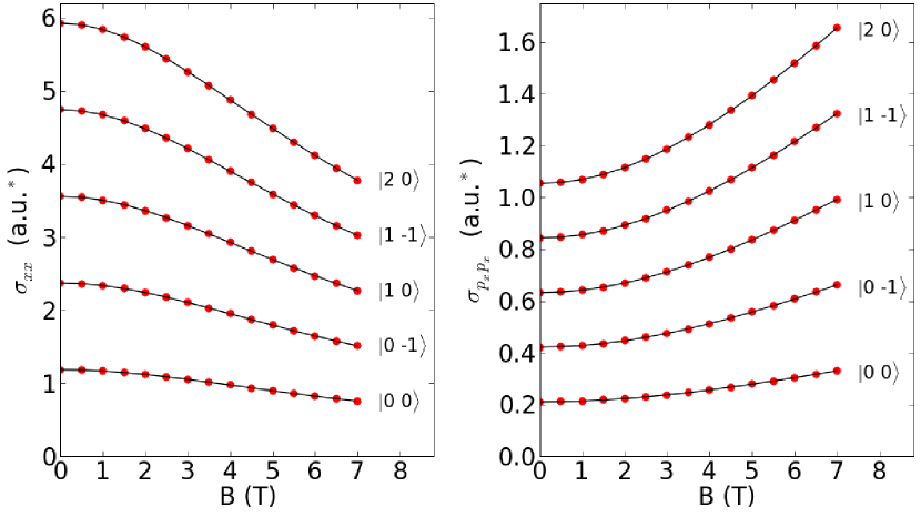
Figure 1: (Color online) Variances in position and momentum shown for some one-electron GaAs quantum dot states $|nm\rangle$, given in effective atomic units: $\sigma_{xx}$ has dimension length², where length is measured in effective Bohr radii ($a_{0}^{*}\approx 9.794\,$nm) and $\sigma_{p_{x}p_{x}}$ is measured in Hartree${}^{*}m^{*}$ where $m^{*}=0.067\,m_{e}$ and Hartree${}^{*}\approx 11.857\,$meV is the effective atomic energy unit.

This behavior can be understood qualitatively by considering a usual one-dimensional harmonic oscillator, where the variances of the $n$-th state are given by $\sigma_{xx}=(1+2n)\hbar/(2m^{*}\omega)$ and $\sigma_{p_{x}p_{x}}=(1+2n)\hbar m^{*}\omega/2$. Physically, this simply means that with increasing magnetic field the electron becomes more localized in position space and less localized in momentum space. The uncertainty relation in each coordinate, however, does not depend on $\omega$ (and hence neither on the magnetic field) since it is determined by the product of the variances:

$$\sigma_{xx}\sigma_{p_{x}p_{x}}-\sigma_{xp_{x}}^{2}\geq\frac{1}{4}$$ (30)

(and in the same way for $y,p_{y}$). Also, for the quantum dot states, the initial covarinaces $\sigma_{xp_{x}}$ and $\sigma_{yp_{y}}$ always vanish. Among all states, it is only the ground state $|nm\rangle=|0\,0\rangle$ that has minimum uncertainty due to its ideal Gaussian shape, while for excited states the Gaussian shape is disturbed and the uncertainty relation becomes a strict inequality. This corresponds to the fact that the ground state of a harmonic oscillator is a particular case of a Glauber coherent state. Hence, $\delta_{D}(t=0)$ must be equal to unity for the quantum dot ground state which agrees with the calculations and retrospectively confirms the imposed definition of the decoherence parameter.

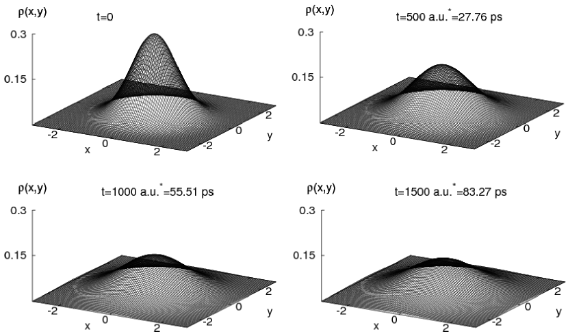
Figure 2: Time evolution of the probability density in coordinate space shown for $B=1\,$T, $T=25\,$K and $\lambda=10^{-3}\omega$ where the dot is initially prepared in the ground state. The coordinates are given in effective Bohr radii $a_{0}^{*}\approx 9.794\,$nm and the probability density in units of $1/(a_{0}^{*})^{2}$.

In addition to the previously discussed initial conditions, also the coupling strength to the environment needs to be determined. As already mentioned in the introduction, the advantage of the model used here is that one can phenomenologically account for, in principle, any kind of environmental effects simply by choosing appropriate values of the phenomenological constants. However, since the master equation (4) is only valid for weak coupling of the reduced system to the environment, the ratio $\lambda/\omega$ should be much smaller than unity, which restricts the model to the description of processes that obey this condition. Here, we consider the dissipative effects to be caused by electron-phonon interactions and therefore the dissipation rate $\lambda$ is approximately given by the electron-phonon scattering rate. The latter ones were found to be typically of the order $\lambda\approx 10\,{\rm ns}^{-1}$ in GaAs structures Bockelmann (1994); Bertoni et al. (2005); Stavrou and Hu (2005); Climente et al. (2006). For the effective confinment strength chosen here, this yields $\lambda\approx 10^{-3}\omega$ and hence the Markovian approach can be seen as justified in the present study. Another aspect to be considered is that, apart from being incorporated in the diffusion coefficients (Eq. 20), the temperature also influences the phonon scattering rate. However, since the phonon scattering rates for different temperatures are not known exactly, the parameter $\lambda$ is varied independently in the relevant region at different temperatures to investigate its influence on the decoherence time scale.

Figure 2 shows the time evolution of the probability density (obtained by setting $x=x^{\prime},\,y=y^{\prime}$ in Eq. (24)) and figure 3 the time evolution of the decoherence degree when the quantum dot is initially prepared in the ground state.

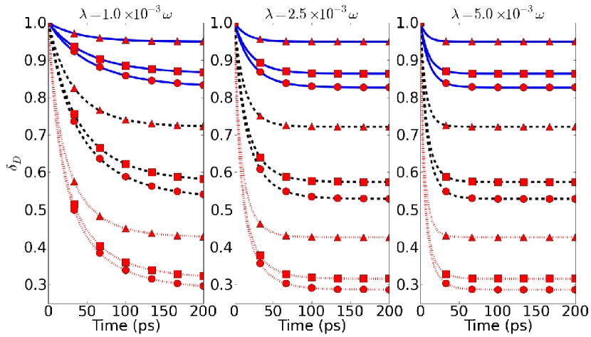
Figure 3: (Color online) Time evolution of the decoherence degree for three different environmental coupling strengths $\lambda$. The solid curves correspond to a temperature of $T=25\,$K, the dashed curves to $T=50\,$K and the dotted curves to $T=100\,$K, while the different magnetic fields are indicated by symbols: $B=1\,$T (circles), $B=3\,$T (squares) and $B=7\,$T (triangles).

We observe that the asymptotic degree of decoherence strongly depends on the temperature and, more weakly, on the magnetic field strength. Naturally, higher temperatures lead to stronger decoherence, while a strong magnetic field has a protective effect on quantum coherence. This corresponds to the result obtained for the one-dimensional case Isar and Scheid (2007), where the asymptotic decoherence degree was shown to be $\delta_{D}(\infty)=\tanh(\hbar\omega/(2kT))$ (Recall that the effective confinement $\omega$ increases with $B$). However, the time scale itself on which the system approaches its asymptotical decoherence is determined by the coupling to the environment. Depending on the latter, decoherence occurs on a time scale between $20-200\,$ps. It is interesting to note that the rule of thumb to estimate the ratio of relaxation ($\tau_{r}$) and decoherence ($\tau_{D}$) time scale Schlosshauer (2007)

$$\frac{\tau_{r}}{\tau_{D}}\approx\left(\frac{\sqrt{\sigma_{xx}}}{L_{dB}}\right)^{2},$$ (31)

where $L_{dB}$ is the thermal de Broglie wave length,

$$L_{dB}=\frac{\hbar}{\sqrt{2m^{*}kT}},$$ (32)

holds in the case studied here, but the ratio is of the order of unity, which is a rather untypical behavior. In fact, in many situations decoherence is several orders of magnitude faster than dissipation and relaxation; For macroscopic systems, the ratio (31) becomes astronomically large Isar and Scheid (2007); Schlosshauer (2007); Zurek (1991). In quantum dots, however, the wave packet spread can be of the same order as the thermal de Broglie wave length - a very remarkable property, once again displaying their fascinating features.

V Conclusions

Using a Markovian master equation approach with linear Lindblad operators, we investigated the dissipative phase space dynamics of a one-electron quantum dot. We obtained the density matrix in coordinate representation from which an expression for the spatial decoherence parameter was derived. With numerically calculated initial values for the first and second moments of a quantum dot in a prepared state, we analyzed the time evolution of decoherence and the influence of the temperature and an external magnetic field. The phenomenological coupling to the environment was assumed to emerge from electron-phonon scattering. We found that the asymptotic decoherence strongly depends on the temperature and also on the magnetic field and the decoherence time scale is driven by environmental coupling strength, varying between a few and a few hundred picoseconds.

The model presented here has the advantage of being rather simple. The price one has to pay is, on the one hand, its phenomenological nature and, on the other hand, the restriction to Markovian dynamics. Hence, the obtained results should be viewed with these limitations in mind. If, for example, one aims to investigate decoherence arising from faster processes than electron-phonon scattering, the weak coupling limit is not necessarily valid, since the dissipation constant approaches the confinement strength. At the same time, the phenomenological nature also has the advantage that one is able to describe different kinds of interactions without loss of generality, just by choosing different values for the emerging constants, as long as the Markovian condition is not violated.

Further difficulties can occur, if, for example, the circular symmetry is disturbed or anharmonic effects have to be accounted for. In that case, the off-diagonal coupling constants in Eqs. (12) or (19) may be non-zero, and it may also be quite non-trivial to find a single decoherence parameter in this case. It should be stressed that analytical solvability is provided for a purely harmonic confinement only, while for more complex potentials even a numerical solution is not always possible, since no finite system of the equations of motions can be derived.

Another conclusion we can draw from the present study is that, if the temperature is very much smaller than the confinement strength ($kT\ll\hbar\omega$), spatial decoherence should not be of significant relevance. Even at a temperature of $25\,$ K we see that the asymptotic decoherence is about $\delta_{D}(t\rightarrow\infty)\approx 0.9$. However, in some experimental setups the temperatures are as low as $T=100\,$mK, and hence we can conclude that spatial decoherence practically does not occur in that case.

As for further applications of the model presented here, it should be also suited to study tunneling processes in quantum dot molecules. Calculations on tunneling through one-dimensional parabolic potentials with dissipation described by linear Lindblad operators were, e.g., demonstrated in Adamian et al. (1998); Isar et al. (2000), which can be extended to the two-dimensional case.

References

- Loss and DiVincenzo (1998) D. Loss and D. P. DiVincenzo, Phys. Rev. A 57, 120 (1998).
- Folk et al. (2001) J. A. Folk, C. M. Marcus, and J. S. Harris, Phys. Rev. Lett. 87, 206802 (2001).
- Htoon et al. (2001) H. Htoon, D. Kulik, O. Baklenov, A. L. Holmes, T. Takagahara, and C. K. Shih, Phys. Rev. B 63, 241303(R) (2001).
- Vagov et al. (2004) A. Vagov, V. M. Axt, T. Kuhn, W. Langbein, P. Borri, and U. Woggon, Phys. Rev. B 70, 201305(R) (2004).
- Sanguinetti et al. (2006) S. Sanguinetti, E. Poliani, M. Bonfanti, M. Guzzi, E. Grilli, M. Gurioli, and N. Koguchi, Phys. Rev. B 73, 125342 (2006).
- Bernardot et al. (2006) F. Bernardot, E. Aubry, J. Tribollet, C. Testelin, M. Chamarro, L. Lombez, P. F. Braun, X. Marie, T. Amand, and J.-M. Gérard, Phys. Rev. B 73, 085301 (2006).
- Khaetskii et al. (2002) A. V. Khaetskii, D. Loss, and L. Glazman, Phys. Rev. Lett. 88, 186802 (2002).
- Khaetskii et al. (2003) A. Khaetskii, D. Loss, and L. Glazman, Phys. Rev. B 67, 195329 (2003).
- Golovach et al. (2004) V. N. Golovach, A. Khaetskii, and D. Loss, Phys. Rev. Lett. 93, 016601 (2004).
- Vorojtsov et al. (2005) S. Vorojtsov, E. R. Mucciolo, and H. U. Baranger, Phys. Rev. B 71, 205322 (2005).
- Jacak et al. (2005) L. Jacak, J. Krasnyj, W. Jacak, R. Gonczarek, and P. Machnikowski, Phys. Rev. B 72, 245309 (2005).
- Thorwart et al. (2005) M. Thorwart, J. Eckel, and E. R. Mucciolo, Phys. Rev. B 72, 235320 (2005).
- Zhang et al. (2006) W. Zhang, V. V. Dobrovitski, K. A. Al-Hassanieh, E. Dagotto, and B. N. Harmon, Phys. Rev. B 74, 205313 (2006).
- Yao et al. (2006) W. Yao, R. B. Liu, and L. J. Sham, Phys. Rev. B 74, 195301 (2006).
- BhaktavatsalaRao et al. (2006) D. D. BhaktavatsalaRao, V. Ravishankar, and V. Subrahmanyam, Phys. Rev. A 74, 022301 (2006).
- Deng and Hu (2006a) C. Deng and X. Hu, Phys. Rev. B 73, 241303(R) (2006a).
- Deng and Hu (2006b) C. Deng and X. Hu, Phys. Rev. B 74, 129902(E) (2006b).
- BenChouikha et al. (2007) W. BenChouikha, S. Jaziri, and R. Bennaceur, Phys. Rev. A 76, 062303 (2007).
- Semenov and Kim (2007) Y. G. Semenov and K. W. Kim, Phys. Rev. B 75, 195342 (2007).
- Jiang et al. (2008) J. H. Jiang, Y. Y. Wang, and M. W. Wu, Phys. Rev. B 77, 035323 (2008).
- Stano and Fabian (2008) P. Stano and J. Fabian, Phys. Rev. B 77, 045310 (2008).
- Zhang et al. (2008) W. Zhang, N. P. Konstantinidis, V. V. Dobrovitski, B. N. Harmon, L. F. Santos, and L. Viola, Phys. Rev. B 77, 125336 (2008).
- Woods et al. (2008) L. M. Woods, T. L. Reinecke, and A. K. Rajagopal, Phys. Rev. B 77, 073313 (2008).
- Yang and Liu (2008) W. Yang and R. B. Liu, Phys. Rev. B 77, 085302 (2008).
- Hernandez et al. (2008) F. G. G. Hernandez, A. Greilich, F. Brito, M. Wiemann, D. R. Yakovlev, D. Reuter, A. D. Wieck, and M. Bayer, Phys. Rev. B 78, 041303(R) (2008).
- Tu and Zhang (2008) M. W. Y. Tu and W. M. Zhang, Phys. Rev. B 78, 235311 (2008).
- Zurek (2003) W. H. Zurek, Rev. Mod. Phys. 75, 715 (2003).
- Waltersson et al. (2009) E. Waltersson, E. Lindroth, I. Pilskog, and J. P. Hansen, Phys. Rev. B 79, 115318 (2009).
- Isar and Scheid (2007) A. Isar and W. Scheid, Physica A 373, 298 (2007).
- Gupta et al. (1984) R. K. Gupta, M. Muenchow, A. Sandulescu, and W. Scheid, J. Phys. G: Nucl. Phys 10, 209 (1984).
- Sandulescu et al. (1987) A. Sandulescu, H. Scutaru, and W. Scheid, J. Phys. A: Math. Gen. 20, 2121 (1987).
- Palchikov et al. (2000) Y. V. Palchikov, G. G. Adamian, N. V. Antonenko, and W. Scheid, J. Phys. A: Math. Gen. 33, 4265 (2000).
- Maksym and Chakraborty (1990) P. A. Maksym and T. Chakraborty, Phys. Rev. Lett. 65, 108 (1990).
- Reimann and Manninen (2002) S. M. Reimann and M. Manninen, Rev. Mod. Phys. 74, 1283 (2002).
- Waltersson and Lindroth (2007) E. Waltersson and E. Lindroth, Phys. Rev. B 76, 045314 (2007).
- Rothman and Mazziotti (2008) A. E. Rothman and D. A. Mazziotti, Phys. Rev. A 78, 032510 (2008).
- Dodonov and Manko (1985) V. V. Dodonov and O. V. Manko, Physica A 130, 353 (1985).
- Kalandarov et al. (2007) S. A. Kalandarov, Z. Kanokov, G. G. Adamian, and N. V. Antonenko, Phys. Rev. E 75, 031115 (2007).
- Anastopoulos and Hu (2000) C. Anastopoulos and B. L. Hu, Phys. Rev. A 62, 033821 (2000).
- Chou et al. (2008) C. H. Chou, T. Yu, and B. L. Hu, Phys. Rev. E 77, 011112 (2008).
- Lindblad (1976) G. Lindblad, Commun. math. Phys. 48, 119 (1976).
- Karrlein and Grabert (1997) R. Karrlein and H. Grabert, Phys. Rev. E 55, 153 (1997).
- Gallis (1996) M. R. Gallis, Phys. Rev. A 53, 655 (1996).
- Haba (1998) Z. Haba, Phys. Rev. A 57, 4034 (1998).
- Isar et al. (1999) A. Isar, A. Sandulescu, and W. Scheid, Phys. Rev. E 60, 6371 (1999).
- Isar and Scheid (2002) A. Isar and W. Scheid, Phys. Rev. A 66, 042117 (2002).
- Dietz (2004) K. Dietz, J. Phys. A: Math. Gen. 37, 6143 (2004).
- Dekker and Valsakumar (1984) H. Dekker and M. C. Valsakumar, Phys. Lett. A 104, 67 (1984).
- Sandulescu and Scutaru (1987) A. Sandulescu and H. Scutaru, Ann. Phys. 173, 277 (1987).
- Adamian et al. (1999a) G. G. Adamian, N. V. Antonenko, and W. Scheid, Nucl. Phys. A 645, 376 (1999a).
- Adamian et al. (1999b) G. G. Adamian, N. V. Antonenko, and W. Scheid, Phys. Lett. A 260, 39 (1999b).
- Wang and Uhlenbeck (1945) M. C. Wang and G. E. Uhlenbeck, Rev. Mod. Phys. 17, 323 (1945).
- Agarwal (1971) G. S. Agarwal, Phys. Rev. A 4, 739 (1971).
- Joos et al. (2003) E. Joos, H. D. Zeh, C. Kiefer, D. Giulini, J. Kupsch, and I. O. Stamatescu, Decoherence and the Appearance of a Classical World in Quantum Theory (Springer-Verlag, 2003).
- Schlosshauer (2007) M. Schlosshauer, Decoherence and the quantum-to-classical transition (Springer-Verlag, 2007).
- Morikawa (1990) M. Morikawa, Phys. Rev. D 42, 2929 (1990).
- Földi et al. (2003) P. Földi, M. G. Benedict, A. Czirjàk, and B. Molnàr, Phys. Rev. A 67, 032104 (2003).
- Friedrich (2006) H. Friedrich, Theoretical Atomic Physics (Springer Verlag, 2006).
- deBoor (1978) C. deBoor, A Practical Guide to Splines (Springer-Verlag, 1978).
- Bockelmann (1994) U. Bockelmann, Phys. Rev. B 50, 17271 (1994).
- Bertoni et al. (2005) A. Bertoni, M. Rontani, G. Goldoni, and E. Molinari, Phys. Rev. Lett. 95, 066806 (2005).
- Stavrou and Hu (2005) V. N. Stavrou and X. Hu, Phys. Rev. B 72, 075362 (2005).
- Climente et al. (2006) J. I. Climente, A. Bertoni, G. Goldoni, and E. Molinari, Phys. Rev. B 74, 035313 (2006).
- Zurek (1991) W. H. Zurek, Phys. Today 44, 36 (1991).
- Adamian et al. (1998) G. G. Adamian, N. V. Antonenko, and W. Scheid, Phys. Lett. A 244, 482 (1998).
- Isar et al. (2000) A. Isar, A. Sandulescu, and W. Scheid, Eur. Phys. J. D 12, 3 (2000).