Viscous shocks in Hele-Shaw flow and Stokes phenomena of the Painlevé I transcendent

Abstract

In Hele-Shaw flows at vanishing surface tension, the boundary of a viscous fluid develops cusp-like singularities. In recent papers [1, 2] we have showed that singularities trigger viscous shocks propagating through the viscous fluid. Here we show that the weak solution of the Hele-Shaw problem describing viscous shocks is equivalent to a semiclassical approximation of a special real solution of the Painlevé I equation. We argue that the Painlevé I equation provides an integrable deformation of the Hele-Shaw problem which describes flow passing through singularities. In this interpretation shocks appear as Stokes level-lines of the Painlevé linear problem.

1 Introduction

Hele-Shaw flow describes a 2D viscous incompressible fluid with a free boundary at low Reynolds numbers. The fluid is driven to a drain by another, inviscid, incompressible liquid or a gas (see e.g., [3]). Under this process the boundary of the fluid evolves in an unstable manner, revealing singularities occurring at a finite time.

The governing equations - Darcy’s law - can be easily derived from Navier-Stokes equations under the assumption of a Poisseuille profile. In units such that the fluid density and hydraulic conductivity are set to one, velocity of the fluid is proportional to the gradient of pressure

$$\mathbf{v}=-\mathbf{\nabla}p.$$ (1)

In incompressible fluids, $\mathbf{\nabla}\cdot\mathbf{v}=0$ and pressure is a harmonic function, $\Delta p=0$, everywhere except at a drain (a marked point set at infinity), where the fluid disappears with a constant flux $Q=\oint_{\infty}\mathbf{v}\times{{d}}\mathbf{\ell}$ i.e. the amount of fluid removed in the time interval ${{d}}T$ is $Q{{d}}T$.

In the regime where the surface tension at the fluid boundary may be neglected, the case we consider, pressure is a constant $p|_{\Gamma}=0$ along the fluid boundary $\Gamma$.

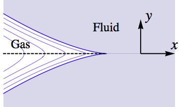
Figure 1: A finger growing in time (sequence of blue lines) toward the (2,3)-cusp singularity. The dashed line is the branch cut of the height function.

The Hele-Shaw problem is just one particular realization of a broad class of growth processes governed by the Darcy law. Darcy law states that the normal velocity of a line element of the boundary $d\ell$ is proportional to its harmonic measure density. Harmonic measure is the probability of a Brownian excursion starting at a marked point (in this case it is a drain) to exit the domain through that boundary element. The probability density of Brownian excursion is the Poisson excursion kernel, equal to the gradient $|\nabla p|$ of a harmonic function $p$ with a source at a marked point and Dirichlet boundary condition.

A well-known stochastic realization of the Darcy law is DLA – diffusion-limited aggregation [4]. It is realized through Brownian excursions of particles with a small size $\hbar$ emanating at a constant rate from a distant point, with absorbing boundary, such that the stopping-set cluster grows. The Darcy law emerges at vanishing particle size, $\hbar\to 0$.

Computer experiments with DLA [4] show that a boundary, initially featureless, very quickly develops into a branching graph with a width controlled by the size of one particle $\hbar$. This signals that the limit $\hbar\to 0$ is impossible.

Darcy’s law (1) also indicates that Hele-Shaw flow tends to a microscale. Non-linear differential equation (1) is ill-defined. A smooth initial boundary first evolves into a fingering pattern, then fingers at a finite, critical time develop cusp singularities [5, 6, 7, 8]. At that point the differential form of the Darcy law stops making sense. This phenomenon constitutes the major problem in the field.

Unlike in fluid dynamics, DLA processes possess a dimensional parameter – the particle size $\hbar$. It plays the role of a minimal area, which regularizes singularities emerging in fluid dynamics.

Comparing Hele-Shaw flows to DLA suggests that, after a singularity is reached, the flow should feature shocks - a graph of curved lines where pressure (and velocity) suffer discontinuities. Such solutions of ill-defined non-linear differential equations are known as weak solutions [9].

In Refrs. [1, 2] we developed the weak solution of Hele-Shaw problem, which we believe to be a solution of the problem of Hele-Shaw singularities. Within this solution, a singularity triggers a branching graph of shocks or cracks propagating through the viscous fluid. Shocks at small Reynolds number is a new phenomena, not yet being observed experimentally. We refer them as viscous shocks. An emerging pattern of viscous shocks is reminiscent DLA patterns.

The weak solution of the Hele-Shaw flow is based on an integral form of the Darcy law. This form of the non-linear equation suggests an interpretation of the Darcy law as an evolution of a real Riemann surface (a complex curve with reality conditions). A singularity signals that the evolving Riemann surface changes its genus.

A similar problem is known in a different field - a slow dynamics of modulated fast oscillatory non-linear waves (see e.g., [10]). If a non-linear wave features a separation of scales, in the form of a slow modulation of fast oscillations, the slow part is described Whitham equations [11, 12]. Conversely, the Whitham equations can be interpreted as the evolution of Riemann surfaces

In Refrs. [1, 2] we described hydrodynamics of shocks initiated by the most generic cusp singularity, referred to as a (2,3)-cusp. In local Cartesian coordinates aligned with a cusp axis, the shape of a critical finger is $y^{2}\sim x^{3}$, as in Fig. 1.

Right before the occurrence of a (2,3)-cusp singularity, a Riemann surface describing Hele-Shaw flow is a sphere. Right after a singularity, the sphere transforms into a torus (or elliptic complex curve). Exactly the same transition appears in a semiclassical approximation of special, often called “physical” solutions of the Painlevé I equation [13, 14].

Appearance of the Painlevé equation in Hele-Shaw dynamics is not accidental. In this paper we clarify this relation. We show that the Hele-Shaw singular flow and emerging shock pattern are directly related to “physical” solutions of Painlevé I equation:

$$u_{ttt}-12uu_{t}=\hbar,$$ (2)

where the Painlevé -function $u(t)$ is a real function for real values of the argument.

As it is seen in Fig. 2, the Painlevé -function behaves drastically different at large negative times $t<0$ and large positive times $t>0$. At $t<0$ the Painlevé -function is smooth. It turns to an oscillatory regime at $t>0$.

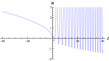
Figure 2: Illustration of a physical Painlevé -function by means of Whitham approximation: at $t<0$ the Painlevé -function is smooth $u\approx\sqrt{-\hbar t/6}$. It features fast oscillations at $t>0$, but the change of the period and amplitude remain smooth. The (orange) dashed line is the envelop of minima $u(t_{n})\approx 0.553594\sqrt{\hbar t_{n}/6}$. The picture captures only the asymptotes at large $|t|$, not a crossover between smooth and oscillatory regimes.

The Painlevé -function may be linked to the position of the tip of the finger $e(T)$. The relation changes while passing through the singularity: at the smooth phase (large negative $T$) the tip progresses as $e(T)=-2u(t)<0,\;T\to-\infty$; at large positive $T$ (after the singularity) the tip retreats, its position follows a slowly moving position of minima of the Painlevé function $e(T)=u(t_{n})<0$, where $t_{n}$ is a sequence of time, labeled by an integer $n$, such that $\dot{u}(t_{n})=0$. In both cases, the relation between a ”slow” time $T$ of the Hele-Shaw flow and a ”fast” time $t$ - an argument of the Painlevé function is

$$T=\frac{\hbar t}{6},\;T<0;\quad T=\frac{\hbar t_{n}}{6},\;T>0.$$ (3)

The Hele-Shaw flow is directly related to the semi-classical ($\hbar\to 0$) limit of the Painlevé “wave-function” $\Psi(X,t)$ – solution of the linear ordinary differential equation associated with Painlevé I equation:

$$\Big{[}\partial_{t}^{2}-2u(t)\Big{]}\Psi=X\Psi.$$ (4)

The argument $X=x+iy$ (complex spectral parameter of the linear problem) plays a role of a complex coordinate of the fluid. Shocks appear as Stokes level lines of the Painlevé wave-function. Hydrodynamic objects are obtained from the wave-function by averaging over fast time oscillations. In particular, pressure reads

$$p(x,y)=-\lim_{\hbar\to 0}{\rm Re}\,\,\hbar\,\partial_{T}\overline{\log\Psi(x+iy,t)}=-6\lim_{\hbar\to 0}{\rm Re}\,\,\partial_{t}\log\Psi(x+iy,t_{n}),$$

where overline means an average over fast time oscillations. Alternatively one can evaluate the wave-function at discrete time moments (3) .

We believe that the relation between the singular Hele-Shaw problem and the Painlevé I equation clarifies both entities. It further explains the nature of weak solutions of Hele-Shaw problem and shocks in viscous fluids, and provides a transparent, hydrodynamic interpretation of a subtle semiclassical description of Painlevé I, which otherwise is rather formal and complicated. In this paper we give a brief account of both sides of the story: the shock-wave solution of the Hele-Shaw flow and the Whitham averaging method for the physical solution of Painlevé I, even though elements for each of these themes taken separately can be found in the literature. We have found that approach to Painlevé -equation as an isomonodromic deformation developed in Refrs. [16, 17, 18, 19, 20, 21] provides the closest connection between Painlevé -equation to Hele-Shaw hydrodynamics.

The appearance of the Painlevé equation in the Hele-Shaw problem is more than a formal analogy. Painlevé equation gives an integral Hamiltonian regularization of the Hele-Shaw singularities anticipated in Ref. [8].

Contrary to the Darcy law, the Painlevé equation (like a DLA process), has a dimensional parameter $\hbar$. The meaning of this parameter can be understood as follows. The physical solution of Painlevé I-equation is selected by the asymptote $u\to+\sqrt{-T}>0$ at large negative times $T\to-\infty$. At large positive times $T>0$, this solution features fast oscillations with a period of the order of $\hbar$. The period of oscillations also changes in time, but slowly, such that the period in units of $\hbar$ is a regular function at $\hbar\to 0$. As such, $u(T)$ does not have a limit at $\hbar\to 0$, but its period (in units of $\hbar$) does. The Hele-Shaw flow arises from the Painlevé equation in the limit when a dimensional parameter $\hbar$ vanishes. It features singularities and discontinuities while the Painlevé equation at $\hbar\neq 0$ does not. At a non-vanishing $\hbar$ shocks are regularized. They appear as spatial narrow regions of width $\sim\hbar^{3/2}$ where pressure and velocity exhibit finite, though sharp, gradients. In this sense, the Painlevé equation provides a regularization of the Hele-Shaw flow, similar to a regularization that provides DLA.

Emergence of singularities in hydrodynamics is typically caused by an invalid approximation made in an original physical problem. Any physical problem of fluid dynamics always carries a dimensional parameter, which regularizes singularities at a microscale. As a result, physical processes are smooth, but may exhibit large gradients in certain regions of time and space. When the microscale parameter $\hbar$ is naively set to zero in the equations, they may become ill-defined and do not have physical solutions in the regime when gradients are large. However, if the parameter is set to zero in the solution (rather then in the equation), solutions retain their meaning but may become discontinuous, exhibiting shocks – weak solutions [9]. This is what happens in the Hele-Shaw problem.

Painlevé equation itself is an example of these phenomena. Setting $\hbar=0$ in the equation reduces it to $-2uu_{T}=1$, whose solution $\sqrt{-T}$ makes sense (i.e., remains real) only at $T<0$. Although at $T>0$ the Painlevé -function has no formal $\hbar\to 0$ limit, its average over the period of fast oscillations or a motion of minima of Painlevé -function does (as it is seen on the Fig. [13]). We will show that this slow motion is equivalent to the weak solution of the Hele-Shaw problem obtained in Refrs. [1, 2].

In many important cases, weak solutions show a great degree of universality – a large class of regularized problems lead to the same weak solution. It is always interesting to determine regularizations that are “minimal” in some sense. In this paper, we suggest that the Painlevé equation provides the “minimal” regularization for generic singularities of the Hele-Shaw problem. It is the only known integrable regularization.

The nature of the physical solution of the Painlevé equation suggests a physical interpretation of the dimensional parameter $\hbar$. The solution suggests that, under the regularization, the inviscid fluid consists of particles with a minimal area $\hbar$. Oscillations reflects a discreetness of particles and a ”corpuscular” nature of the problem. This interpretation links the Painlevé I regularization of the Hele-Shaw flow with the DLA process where particles are essentially discrete, and provides an analytical basis to study the latter.

In the next section we briefly review the Hele-Shaw critical fingers in terms of evolution of the real complex curve. It provides a necessary language to link the flow with the Painlevé wave-function described in the sequel. Our approach is based on isomonodromy property of Painlevé -equation. Our approach is somewhat different that in the Refrs. [17, 19, 20, 21]. In particular we give a new simple derivation of the expression for the phase (47) and the next leading oscillatory corrections (64),(65) in Sec. refMKB .

A comment on related studies is in order. In Refrs. [22, 23] Hele-Shaw flow has been linked to normal random matrix ensembles, and through them to certain asymptotes of bi-orthogonal polynomials. Random matrix ensembles provide an equivalent regularization scheme of Hele-Shaw flow. Painlevé equation can be formally derived from this approach [23, 24]. In a similar manner Painlevé equation appears in studies of Hermitian random matrix ensembles [25] and related to their asymptotes of orthogonal polynomials [26, 27]. From this perspective a singular Hele-Shaw flow is linked to a distribution of zeros of orthogonal and bi-orthogonal polynomials and eigenvalues of random matrices. In this paper we do not elaborate this approach in order to reduce the size of the paper.

We also comment that an idea that near-cusp structure should be followed by a crack propagation into the fluid domain has been suggested in earlier works [28, 29]. The mechanism discussed in these papers seems different from that in [1, 2].

2 Singularity and viscous shocks

2.1 Evolving complex curve

The flow near a singular finger tip does not depend on details of a boundary away from the tip of the finger. It is sufficient to consider a finger with a symmetry axis. In Cartesian coordinates aligned with a finger axis (Fig. 1), a finger is given by a graph $\pm y(x)$. We recall a description of a viscous finger in terms of the height function $Y(X,T)$ [8]. It is defined as an analytic function on a finite part of the complex plane $X=x+iy$ cut along the symmetry axis of the finger, such that the boundary values are real and equal to the graph of the finger $Y(X)_{X=x+\pm{{i}}0}=\pm y(x,T)$. Darcy law can be expressed through the height function [8]:

$$\partial_{T}Y=-\partial_{X}\phi,$$ (5)

where the analytic function $\phi(X)=\psi+{{i}}p$ is a complex potential of the flow, $\psi$ is a stream function, and $p$ is the pressure.

The height function $Y(X,T)$ defines a complex curve (or Riemann surface) evolving in time. Since at real $X=x$ the height $Y=\pm y(x)$ is real, the curve is real: $\overline{Y(X)}=Y(\overline{X})$.

In Ref.[8] it has been shown that in general the complex curve is hyperelliptic, i.e., $Y^{2}(X)$ is a polynomial of an odd degree. Its degree is preserved while the coefficients evolve in time.

The flow potential $\phi(X)$ has an important interpretation. Darcy law states that $\phi$ is a local parameter of the curve. This means the following: the potential $\phi(X)$ is an analytic function. Locally it can be inverted, so that $X$, and other physical quantities, say, the height function, become functions of $\phi$. Then Darcy law (5) states that functions $\left(Y(\phi),\,X(\phi)\right)$ treated as functions of the potential, are regular and single-valued. In the case of critical flow, when $(Y,\,X)$ is hyperelliptic, the variable $\phi$ covers the physical plane twice: $\phi$ and $-\phi$ correspond to the same $X$, such that the double-valued function $Y(X)$ becomes a single-valued function $Y(\phi)$ on the double covering.

The fact that the potential is a local parameter of the curve is the essence of the Darcy law. The law can be formulated entirely in terms of the curve: the curve $(Y,\,X)$, with a local parameter $\phi$, moves in time such that the differential ${{i}}{{d}}\Omega=Y\,{{d}}X+\phi\,{{d}}T$ is closed. In this form Darcy law becomes identical to Whitham equations describing slow modulation of fast oscillating non-linear waves [10, 30, 12]. This fact was recognized in [15].

A consequence is Polubarinova-Kochina equation [31, 32] (which in modern literature is called “semiclassical string” equation [33] ). Treating $Y$ and $X$ as functions of the complex potential $\phi$, the Darcy law (8) reads

$$\{X,\,Y\}=1,$$ (6)

where the brackets are defined via $\{X,\,Y\}=\partial_{T}X\partial_{\phi}Y-\partial_{\phi}X\partial_{T}Y$ and time derivative is taken at fixed $\phi$.

The flow is best described by a generating function – a central object of this study:

$$\Omega(X)=-{{i}}\int_{e}^{X}Y{{d}}X,$$ (7)

where the integration starts at the tip of the finger $e$ and goes through the fluid. Then the Darcy law reads

$$\partial_{T}\Omega={{i}}\phi.$$ (8)

2.2 Integral form of Darcy law

Darcy law can be equivalently expressed by integration of the differential ${{d}}\Omega$ along various paths in the fluid. Let us integrate (5) over a closed path $B$ in the fluid:

$$\frac{{{d}}\,\,}{{{d}}T}{\rm{Im}}\,\oint_{B}{{d}}\Omega = \!\!\oint_{B}\mathbf{v\times d\ell}=\oint_{B}{{d}}\psi,$$ (9)

$$\frac{{{d}}\,\,}{{{d}}T}{\rm{Re}}\,\oint_{B}{{d}}\Omega = -\oint_{B}\,\mathbf{v\cdot d\ell}=-\oint_{B}{{d}}p.$$ (10)

The imaginary part measures a flux of fluid through the closed path. If the path goes around a drain (infinity), the integral ${\rm{Im}}\,\oint_{B}{{d}}\Omega$ counts a mass of fluid drained up to time $T$. It is $QT$. In a canonical anti-clockwise orientation this reads

$${{i}}\frac{{{d}}}{{{d}}T}\oint_{\infty}{{d}}\Omega=Q>0.$$ (11)

The real part measures circulation along the path. It follows from the differential form of the Darcy law (1), valid before a singularity, that the fluid is irrotational $\mathbf{\nabla\times v}=0$ and therefore $\frac{{{d}}}{{{d}}t}{\rm{Re}}\,\oint_{B}{{d}}\Omega=0$. Therefore ${\rm{Re}}\,\oint_{B}{{d}}\Omega=0$ is a constant. Provided that the constant does not depend of the choice of the path, the constant can be determined by taking the integral around a drain where $\oint_{\infty}{{d}}\Omega$ is purely imaginary as is in (11). Thus ${\rm{Re}}\,\oint_{B}{{d}}\Omega=0$ on any contour in the fluid.

If there are shocks, the height function and ${{d}}\Omega$ jump through a shock. The condition ${\rm{Re}}\,\oint_{B}{{d}}\Omega=0$ for a path crossing a shock must be understood as a sum of the integral over a path in the fluid plus an oriented jump of ${{d}}\Omega$ at points where the path crosses a shock. A proper way to write this condition is to extend the integration over the Riemann surface $(Y,\,X)$ where the height function and the differential ${{d}}\Omega$ are smooth. The physical plane where the hight function suffers a discontinuity consists onn patches of different sheets of the curve. Then the above condition reads

$${\rm{Re}}\,\oint_{B}{{d}}\Omega=0,\quad\rm{any\;cycle\;on\;the\;curve.}$$ (12)

Curves with condition (12) are rather restrictive. We call them Krichever-Boutroux curves. They appeared in seemingly different, but related subjects: random matrix theory [25], asymptotes of orthogonal polynomials [34] and Painlevé transcendents [35, 36, 37].

Eqs. (11,12) combined give a compact and complete formulation of the Hele-Shaw problem: find an evolution of a real Krichever-Boutoux curve (condition (11)), of a given degree, with respect to its residue (time $T$) at a marked point (condition (11)).

Contrary to the differential form of the Darcy law (1), Eqs. (11,12) extend beyond singularities. They admit a weak solution with shocks. Shocks are curved lines where patches of the complex curve covering the physical plane are joined together. At these lines, the height function jumps. Condition (12) being specified for a contour going along both sides of a shock reads

$$\rm{Re}\,\rm{disc}\,\Omega|_{\rm{shocks}}=0.$$ (13)

These conditions determine position and motion of shocks. These are the results of Refs. [1, 2].

In the next two sections we demonstrate how these conditions determine the most generic singularity and also physical solution of the Painlevé I equation.

2.3 (2,3)-singularity and a self-similar elliptic curve

Painlevé I equation is related to the most generic (and the most important) singularity – the (2,3) cusp, where locally the graph of the finger is $y^{2}\sim x^{3}$. In this case a finger is especially simple [8]: $Y^{2}$ is a polynomial of the third degree - an elliptic curve having one branch point at infinity. Fixing a scale and the origin, the curve reads:

$$-Y^{2}=4X^{3}-g_{2}X-g_{3}=4(X-e)(X-e_{2})(X-e_{1}),$$ (14)

where $g_{2}$ and $g_{3}$ are real time dependent coefficients. One of the branch points of the curve (14) may always be chosen real. We denote it as $e$. It is the tip of a finger, where $y(e)=0$. The other two are conjugated $e_{1}=\bar{e}_{2}$ (condition (12) excludes a possibility of real $e_{1}$ and $e_{2}$ - in this case $\rm{disc}\,{{d}}\Omega$ through the branch cut connecting $e_{1}$ and $e_{2}$ is real and does not change sign, so that ${\rm Re}\,\oint_{e_{1},e_{2}}{{d}}\Omega$ can not vanish). This is a real elliptic curve with a negative discriminant $g_{2}^{3}-27g_{3}^{2}<0$. The coefficient $g_{2}$ is determined by the drain rate. Eq. (11) gives $Q\sim\dot{g}_{2}$. We set the rate $Q$ such that

$$g_{2}=-12T.$$ (15)

In this setting the time counts from a cusp event $-Y^{2}=4X^{3}$ occurring at a critical time $T=0$. A real coefficient $g_{3}$ is determined by the condition (12).

This is the simplest curve arising in singular flow. Its distinctive property is self-similarity. As it follows from (11),(12)

$$Y(X,T)=|T|^{3/4}Y\left(|T|^{-1/2}X,1\right),$$ (16)

where $Y(X,1)$ is a unique universal function with no free parameters.

The scaling property alone is sufficient to express $\Omega$ through the height function and potential:

$$\Omega(X)=-{{{i}}}\int_{e}^{X}Y\,dX=-\frac{2\rm i}{5}(XY-2T\phi).$$ (17)

We briefly describe this curve following Refs. [1, 2].

2.4 Smooth flow and a degenerate curve

At $T<0$, before the singularity, the flow is smooth, there are no discontinuities. This follows also from the condition (12). At $g_{2}>0$ only degenerate elliptic curve whose discriminant vanishes, $g_{2}^{3}=27g_{3}^{2}$. The only unknown coefficient is thus determined, $g_{3}=-8(-T)^{3/2}$. The two branch points coincide to a real double point: $e_{1}=e_{2}=+\sqrt{-T}>0$. Then $e=-2e_{1}=-2\sqrt{-T}$. The degenerate curve

$$Y^{2}=-4\left(X-e\right)\left(X+\frac{e}{2}\right)^{2},\quad e=-2\sqrt{-T},\quad T<0$$ (18)

represents a torus with one pinched cycle. The real period of the curve is infinite, the imaginary half-period is $\int_{e}^{-\infty}\frac{dX}{Y}=\pi{{i}}\sqrt{12}(-T)^{-1/4}$. This is a general situation - a continuous flow corresponds to a degenerate curve where all cycles but one are pinched [8] (the number of non-degenerate cycles is equal to the connectivity of the fluid boundary [15]). Condition that all cycles located in the bulk of the fluid are pinched follows from incompressibility of the fluid. Only in this case the fluid potential $\phi$ is analytic.

Alternatively, we notice two holomorphic functions $Y(\phi)$ and $X(\phi)$ with an asymptote $Y^{2}\sim X^{3}$ at large $X$ are polynomials of the third and second degree, respectively. The Darcy law in the form of (6) determines the polynomials

$$X=-\left(\frac{\phi}{6}\right)^{2}+e(T),\quad Y=2\left(\frac{\phi}{6}\right)^{3}-3e(T)\left(\frac{\phi}{6}\right),$$ (19)

and yields to a differential equation for time dependence of the coefficients

$$e\partial_{T}e=-2,$$ (20)

which prompts (18). Real solution exists only at $T<0$.

2.4.1 Beyond singularity: Genus transition.

A finger becomes a cusp when the branch point $e$ and the double point $-\frac{e}{2}=e_{1}=e_{2}$ merge to a triple point $e=e_{1}=e_{2}=0$

$$Y^{2}=-4X^{3},\quad T=0.$$ (21)

After the critical time $g_{2}=-{12}T<0$, the curve is not degenerate. The double point splits into two branch points $e_{1}\neq e_{2}=\bar{e}_{1}$. No smooth solution is possible. The branch points appear in the fluid as endpoints of shocks. Fig. 4 illustrates the genus transition. A pinched cycle of the torus now opens.

The condition (12) requires that the integral over a new cycle be purely imaginary

$$\Omega(e_{1})=\int_{0}^{e_{1}}\sqrt{4X^{3}-g_{2}X-g_{3}}\,{{d}}X=\mbox{imaginary}.$$ (22)

Exactly the same equation has been appeared in works of P. Boutroux [35] on Painlevé I equation. We will refer it as Boutroux condition. This equation can be simplified: since $Y(e_{1})=0$, scaling properties (17) yield that at the end of a shock $e_{1}$, pressure $\phi(e_{1})=0$ also vanishes. The latter uniquely determines the only unknown parameter $g_{3}(T)$ of the curve.

Figure 3: Stokes-level (dashed-blue) lines ${\rm Re}\,\Omega=0$ and Stokes lines (solid black) ${\rm Im}\,\Omega=0$ on the fundamental domain of the double covering of the physical plane. The blue-shaded region maps to the upper half-plane in the physical plane. The other shaded region maps to the lower half-plane.

Let us parametrize the curve $Y(X)$ by a uniformizing coordinate $\lambda$ as

$$X=\wp(\lambda|\,\omega(T),\bar{\omega}(T)),\quad Y={i}\wp^{\prime}(\lambda|\,\omega(T),\bar{\omega}(T))$$ (23)

and compute potential of the flow from the Darcy’s law and scaling property (16)

$$-i\partial_{T}\Omega=\phi(X)=6{{{i}}}\left(\zeta(\lambda)+\frac{g_{3}}{8T}\lambda\right).$$ (24)

Here $\wp$ and $\zeta$ are the elliptic functions of Weierstraß, whose complex conjugated half-periods $\omega(T)=T^{-1/4}\omega(1)$ and $\overline{\omega(T)}$ are yet to be determined. The rhombus-shaped fundamental domain is depicted in Fig. 3.

Conditions that pressure vanishes at $e_{1}$ and formula (24) give the defining equation:

$$\frac{3g_{3}}{2g_{2}}=\frac{\eta+\bar{\eta}}{\omega+\bar{\omega}},$$ (25)

where $\omega+\bar{\omega}$ is a real period of the curve and $\eta=\zeta(\omega)$.

The solution of this equation is found in [13]

$$g_{3} = |T|^{3/2}\left\{\begin{array}[]{lr}-8,&\quad T<0,\\ -7.321762431\dots,&\quad T>0.\end{array}\right.$$ (28)

$$\omega = T^{-1/4}(0.7426778188+i\,0.6070379047).$$ (29)

The genus transition is characterized by an abrupt change of $g_{3}$. The modular invariant of the non-degenerate curve $\frac{g_{2}^{3}}{g_{2}^{3}-27g_{3}^{2}}=6.15870507\dots$ is a unique transcendental number.

2.5 Motion of the finger

The finger is described by the real section of the curve $Y,X$, i.e., by the graph $y(x)=Y(X)$ where $X=x\leq e(T)$. As it follows from the (18) a finger grows and its tips moves to the right as its approaches toward a cusp singularity. After the singularity, the finger retreats, moves to the left and triggers two shocks growing to the right. The tip of the finger gives the position of the branch cut extended toward $-\infty$. The scaling property shows that tip of the finger moves as $\sqrt{|T|}$ but with an abrupt change of the coefficient [1, 13]

$$e(T)=\left\{\begin{array}[]{lr}-2\sqrt{-T},&\quad T<0,\\ -0.553594\sqrt{T},&\quad T>0.\end{array}\right.$$ (30)

In the next section we show that the envelope of the Painlevé function behaves in a similar manner

$$u(T)=\left\{\begin{array}[]{lr}-\frac{1}{2}e(T)=\sqrt{-T},&\quad T<0,\\ \;\;\;\;\;e(T)=-0.553594\sqrt{T},&\quad T>0.\end{array}\right.$$ (31)

2.6 Shocks and Stokes level-lines lines.

Shocks are lines of discontinuity of the generating function $\Omega$, the height function $Y$ and the potential $\phi$. They are selected by the condition (13), which in the case of simple branch points says that shocks are a subset of zero level lines ${\rm Re}\,\Omega=0$. We refer to the lines ${\rm Re}\,\Omega=0$ as Stokes level-lines. There are a total of seven Stokes level-lines connected at branch points. They are transcendental, computed numerically, and depicted on the right panel in Fig. 4, denoted by $\Gamma_{1},...,\Gamma_{7}$.

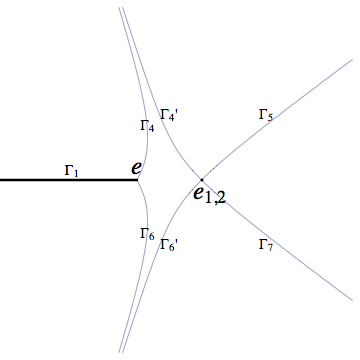
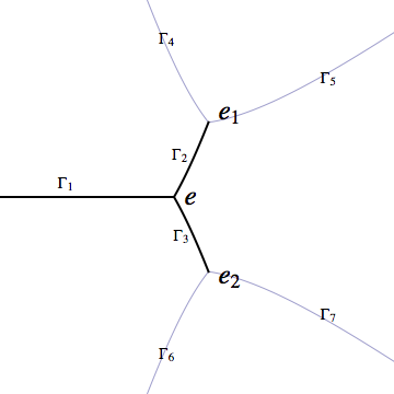
Figure 4: Geometry of Stokes-level lines (black solid lines) before (left panel) and after (right panel) transition. Before the transition four level lines emanate from the double point and end at infinity, neither one is a shock. After the transition the double point splits into two branch points. Condition ${\rm Re}\,\Omega>0$ on the remote part of the finger ${\rm arg}\,X=\pi,\;|X|\to\infty$ uniquely determines configuration of shocks $\Gamma_{3},\Gamma_{2}$. They are always located in the finite part of the plane.

Among the seven Stokes level-lines, only two $\Gamma_{3},\Gamma_{2}$ are shocks. Both sides of the line $\Gamma_{1}$ are boundaries of the finger.

Selection of shocks works as follows. We assume that a remote part of the finger (${\rm arg\,X}=\pi,\;|X|\to\infty$) is not affected by the transition. Therefore at large $X$ the height function $Y(x)$ jumps only on the finger, i.e., on the negative part of real axis. This excludes Stokes level-lines lines $\Gamma_{4,5,6,7}$ ending at infinity. Thus $Y$ jumps only on finite Stokes-level lines $\Gamma_{2,3}$. On a shock, $Y$ (as a complex vector) is orthogonal to the shock. This uniquely determines the shape of shocks (Fig. 4).

The left panel in Fig. 4 represents Stokes level-lines before the transition $T<0$. There are 9 lines. Four Stokes level-lines $\Gamma_{4}^{\prime},\Gamma_{5},\Gamma_{7},\Gamma_{6}^{\prime}$ emanate from the double point. All of them end at infinity. Neither of the Stokes level lines is a shock.

Having in mind the connection to the Painlevé wave-function discussed in the next section, it is useful to translate the selection rule in terms of the generating function: the signs of ${\rm Re}\,\Omega$ are opposite on both sides of $\Gamma_{4,5,6,7}$, and signs are positive on both sides of $\Gamma_{1},\Gamma_{2},\Gamma_{3}$. This is a general situation: Stokes-level lines ${\rm Re}\,\Omega=0$ are shocks if ${\rm Re}\,\Omega$ has the same sign (positive) in the proximity of both sides of a shock [1, 2]

$${\rm Re}\,\Omega|_{X\to\rm{shocks}}>0,\quad{\rm Re}\,\Omega|_{X\in\rm{shocks}}=0.$$ (32)

In the next section we show how the same objects appear in the context of non-linear Stokes phenomenon for the Painlevé I equation.

3 Hele-Shaw flow and physical solution of Painlevé I

3.1 Linear problem for Painlevé I

Painlevé I equation arises as a result of compatibility of two linear differential equations satisfied by the“wave-function” $\Psi(X,t)$ – a central object of this study.

Let $\hat{X}$ and $\hat{Y}$, defined through

$$\hat{X}=\partial_{t}^{2}-2u(t),\quad-i\hat{Y}=-2\partial_{t}^{3}+6u\partial_{t}+3u_{t}$$ (33)

be two Hermitian differential operators. Then the linear problem reads

$$\hat{X}\Psi=X\Psi,\quad\hat{Y}\Psi={{i}}\hbar\partial_{X}\Psi.$$ (34)

The two equations are compatible only if $u(t)$ obeys Painlevé I equation $u_{tt}-6u^{2}=\hbar t.$ Only then

$$[\hat{X},\,\hat{Y}]=-i\hbar,$$ (35)

as it follows from (34).

3.2 Painlevé equation as a quantized Hele-Shaw flow

Equation (4) and (33) are to be compared with (6) and (19) describing a smooth Hele-Shaw flow. One identifies the operators $\hat{X},\,\hat{Y},\,\hat{\phi},\,u$ with their classical counterparts $X,\,Y,\,\phi,\,-e$, where we define $\hat{\phi}:=-{{i}}\hbar\partial_{T}=-6i\partial_{t}$. From this point of view Painlevé equation is seen as a quantization of Hele-Shaw problem, when the brackets in (6) are replaced by the commutator in (4): $\{\,,\,\}\to\frac{i}{\hbar}[\,,\,]$. The quantization introduces a new parameter $\hbar$ which regularizes singularities of the flow. It will be sent to zero when a solution is found. This point of view has been suggested in [8].

As we discussed in the introduction, the limit $\hbar\to 0$ exists only before a flow reached a singularity. After this point solution oscillates and formally does not have a limit. However its average over the period of oscillations does.

Quantization suggests a regularizing scheme for the Hele-Shaw flow: observables in the classical flow are diagonal matrix elements of the corresponding operators averaged over the period of oscillations. One may consider the height function, flow potential, and velocity of a regularized flow defined as an expectation value of corresponding operators averaged over the period

$$\langle\hat{Y}\rangle:=\overline{\Psi^{-1}\left({{i}}\hbar\partial_{X}\right)\Psi},$$

$$\langle\phi\rangle:=\overline{\Psi^{-1}\left(-{{i}}\hbar\partial_{T}\right)\Psi,}$$ (36)

$$\langle v\rangle:=\overline{\Psi^{-1}\left({{i}}\hbar\partial_{T}\partial_{X}\right)\Psi},$$

where $\overline{\cal O}=({\rm period})^{-1}\oint{\cal O}dt$ is an average over the period. These quantities have a regular (asymptotic) expansion in $\sqrt{\hbar}$.

In the remaining part of the paper we will show that a semiclassical limit of the physical Painlevé wave-function describes the Hele-Shaw flow before and after a singularity. This statement is summarized as: the generating function $\Omega=-{{i}}\int^{X}YdX$, (7) of the flow is the Hamilton-Jacobi action of the semiclassical approximation

$$\Omega=\lim_{\hbar\to 0}\hbar\,\overline{\log\Psi(X,t)}.$$ (37)

3.3 Physical wave-function and asymptotes at infinity

The general solution of the Painlevé equation is a two-parametric family. Among them we must select a physical solution which we corresponds to the Hele-Shaw flow by means of (37). A central physical principle we have already used as a guideline is: flow around a finger does not affect the flow at infinity. The height function and the potential are holomorphic functions around infinity (the drain) $\phi\sim-6{{i}}X^{1/2},\,Y\sim 2{{i}}X^{3/2}$ at $X\to\infty,\;|\mbox{Arg}X|<\pi$, as it follows from (19). In terms of the wave function, these conditions read: the asymptote of the physical wave-function at infinity is an analytic function in the plane cut along the finger $\mbox{Arg}X=\pi$

$$\hbar\log\Psi|_{X\to\infty}=\Omega|_{X\to\infty}\to\frac{4}{5}X^{5/2}-t\,X^{1/2},\quad|\mbox{Arg}|X<\pi.$$ (38)

Also, we must impose two additional conditions. One is reality

$$\overline{\Psi(X)}=\Psi(\overline{X}).$$ (39)

The second is that at $t=6T/\hbar\to-\infty$ the Boutroux condition (12) holds

$$\lim_{\hbar\to\infty}\hbar\,{\rm Re}\,\oint{{d}}\log\Psi=0,\quad t\to-\infty.$$ (40)

As a consequence

$$u(t)\to-\frac{e(T)}{2}=\sqrt{-T}=\sqrt{-\frac{\hbar t}{6}}>0,\quad t\to-\infty$$ (41)

where $e(T)$ is a coordinate of the tip of the finger and $e(T)/2$ is a position of the double point.

These simple requirements determine both the physical Painlevé function and the physical Painlevé wave-function.

3.4 Viscous shocks and Stokes phenomena of Painlevé transcendent

The Painlevé wave-function is an entire function. It is differentiable everywhere in $X$. However, its semiclassical limit is not. The gradient $\Psi^{-1}\hbar\,\partial_{X}\Psi$ is of order one in most part of the plane, except some lines where it changes abruptly on a scale vanishing with $\hbar$ across these lines. At $\hbar\to 0$ sharp gradients become discontinuities - seen as shocks in viscous flow. The origin of these lines is simple: they go through the locus of zeroes of the wave-functions. Zeros are separated by $\hbar$ (at the end of the line the separation is $\hbar^{2/3}$), and at $\hbar\to 0$ accumulate to a line distribution. Gradients through lines of zeroes are large.

Discontinuity of the semiclassical approximation of analytic functions is known as Stokes phenomenon. The locus of zeroes is closely related to Stokes phenomena. Shocks occur on some Stokes level-lines selected by the condition (32) and described in more details in the sequal.

The governing conditions (39) and (38) determine the Stokes multipliers and semiclassical wave-function.

4 The physical solution of Painlevé I transcendent

Among many solutions of Painlevé I equation

$$u_{tt}-6u^{2}=\hbar t$$ (42)

called Painlevé functions (see e.g.,[38, 17]), we look for the solution which at $t\to-\infty$ corresponds to a smooth Hele-Shaw flow as in (41). This correspondence also establishes a relation (3) between the time of the Hele-Shaw flow $T$ and the argument of Painlevé -function $t$ a relation between times . The correspondence selects a one parametric family of Painlevé -functions. Following [14] we call this solution “physical” (it is also known as “separatrix” [17] ).

This solution is scale invariant under the rescaling

$$u\to\delta^{-2/5}u,\,t\to\delta^{-4/5}t,\,u_{t}\to\delta^{-3/5}u_{t},\,\hbar\to\delta\hbar.$$ (43)

Below we review some major facts about asymptotes of the physical Painlevé -functions and derive most of them.

4.1 Smooth regime $t\to-\infty$

The sign of the asymptote $u|_{t\to-\infty}>0$ fixes the coefficients of the asymptotic series

$$u(t)-\frac{|e(T)|}{2}=-\frac{|e(T)|}{2}\sum_{k=1}a_{k}(-t)^{-5k/2},\quad t\to-\infty,$$ (44)

where $e(T)$ is given by (41) and $t=6T/\hbar$.

The coefficients $a_{k}$ can be computed recursively, $a_{1}=\frac{1}{48}$. They have a topological meaning as intersection numbers of curves on Riemann surfaces [39], and grow as $a_{k}\sim\frac{1}{\pi^{3/2}}\left(\frac{6}{5}\right)^{1/2}\left(\frac{2^{5}}{5}\sqrt{6}\right)^{-k}\left(2k\right)!$ [18, 40, 20].

The asymptotic series alone does not fix the Painlevé function. A one-parametric family of solutions shares the same series, but differs by the amplitude of an exponentially small correction: consider a difference between two different solutions sharing the same power series $u_{1}$ and $u_{2}$. It obeys the equation $(u_{1}-u_{2})_{tt}=6(u_{1}+u_{2})(u_{1}-u_{2})$. Replace $u_{1}+u_{2}$ by the power series, and solve the linear equation with respect to $u_{1}-u_{2}$. In the first approximation we obtain $(u_{1}-u_{2})_{tt}\approx-12e(T)(u_{1}-u_{2})$. The large (negative) time asymptote is controlled by the WKB approximation:

$$u_{1}-u_{2}\sim\,e(T)\frac{e^{-\frac{4}{5}\sqrt{-6e(T)}(-t)}}{\sqrt{2\pi\sqrt{-6e(T)}(-t)}}$$

This formula is valid in the sector $|{\rm Arg}\,t-\pi|\leq\frac{3\pi}{5}$ if $(-t)$ here and in (41) is understood as $e^{-{{i}}\pi}t$ on the complex plane of $t$ cut along the negative real semi-axis.

Along Stokes level lines $\mbox{Arg}\,t=\pi\mp\frac{2\pi}{5}$ in the complex plane of $t$ at $|t|\to\infty$ the exponential term becomes of order one. There the asymptote of the physical Painlevé -function reads [17, 37, 20, 18]

$$u(t)+\frac{e(T)}{2}\approx-\frac{e(T)}{2}\frac{C\mp\frac{{{i}}}{2}}{2}\frac{e^{-\frac{4}{5}\sqrt{-6e(T)}(-t)}}{\sqrt{2\pi\sqrt{-6e(T)}(-t)}},\quad\mbox{Arg}\,t=\pi\mp\frac{2\pi}{5}$$ (45)

where a real parameter $C$ uniquely characterizes the solution (these formulas are written in a form emphasizing slow and fast time dependence $e(T)=-2(e^{i\pi}\hbar t/6)^{1/2}$). The amplitude $C\pm{{i}}/2$ jumps through the negative part of the real axis. The jump is imaginary and is the same for all physical solutions. The jump is linked to the large order behavior of the coefficients of the asymptotic power series (44) and can be obtained through the Borel transformation technique [18].

4.2 Oscillatory regime: $t\to+\infty$

As $t\to+\infty$ the family of solutions features fast oscillations with a period of order $\hbar$, and has infinite number of double poles clustering at infinity as shown in Fig.2 (there are other double poles in the complex plane of time). Semiclassical description of the solution at $t\to\infty$ is based on a separation of scales between fast oscillations and the slow-varying period. Separation of scales is controlled by the parameter $\hbar$, or large $T$.

At positive large time, the physical Painlevé functions are asymptotically Weierstrass elliptic function

$$u(t)\approx\wp\left(\frac{4}{5}t-\theta(T)|\,\omega(T),\bar{\omega}(T)\right),\quad T=\frac{\hbar}{6}t\to+\infty.$$ (46)

The complex conjugated periods of the Weierstarass function and the phase $\theta(T)=$ slowly depend on time and in the leading approximation do not depend on $\hbar$ [35].

The periods are determined by the Boutroux condition [35] (see (51) below) which happens to be identical to the integral formulation of the Darcy law (12),(22) and is given by (29). Eq.(46) valid at complex time in a sector bounded by Stokes lines $\mbox{Arg}\,t=\pm\frac{\pi}{5}$.

A value of the phase depends on the solution chosen. If one choses to characterize the Painlevé -function by the constant $C$ in (45), one can also characterize the phase by $C$. Relation between $C$ and $\theta$ links asymptotes of Painlevé -function at $T<0$ and $T>0$. It is called connection formula and obtained in Refrs. [37, 19]. Connection formula could be best expressed through the monodromy data $\Phi$ - a (locally) time independent constant defined below in Sec.5.4

$$\pi\theta=\Phi\bar{\omega}+\bar{\Phi}\omega,\quad C=-{\rm Im}\,e^{-{{i}}\Phi},\quad 2{\rm Re}\,e^{{{i}}\Phi}=-1.$$ (47)

The phase $\theta$ is understood through initial data for Painlevé equation. As it follows from (46), at times

$$\frac{4}{5}t_{n}=\theta+(2n+1)(\omega+\bar{\omega}),$$ (48)

where $n$ is a large positive integer, the Painlevé -function reaches the minima $u_{t}(t_{n})=0$ as in Fig. 2. At those points the value of the solution $u(t_{n})\to e(T)$, where $e(T)$ is a real branch point of the Krichever-Boutrox elliptic curve (30).

Scale invariance (43) implies that the periods behave as $|T|^{-1/4}$ (29). Taking this into account the formula (46) reads

$$u(t)\approx\left(\frac{\hbar t}{6}\right)^{1/2}\wp\left[\frac{4}{5}t\left(\frac{\hbar t}{6}\right)^{1/4}-\theta(1)\Big{|}\,\omega(1),\bar{\omega}(1)\right],\quad t\to+\infty,$$ (49)

where $\theta(1),\;\omega(1)$ are just numerical constants.

We will derive all the formulas of the oscillatory regime below. Connection formula (47) requires a more subtle analysis and we do not discuss here.

4.3 Adiabatic invariant and Boutroux condition

Painlevé equation can be interpreted as mechanics of a particle with a coordinate $u$ moving in a potential $-2u^{3}$, under slowly changing force $\hbar t$. At $t\to-\infty$ the particle with a vanishing velocity is located in the unstable position where the force equilibrates the potential as it follows from (41). From there as time progresses the force no longer equilibrates the particle. The particle moves to infinity, but returns from there at a finite time, performing an oscillatory motion.

In oscillatory regime the r.h.s. of the Painlevé - equation (42) is a “slow time” $T$, barely changing over many periods of oscillations. Treating the r.h.s. of (42) as a parameter, the equation becomes an identity for the Weierstrass elliptic function $\wp^{\prime\prime}-6\wp^{2}=-\frac{g_{2}}{2}$, where $g_{2}=-12T$. This gives (49), where the Weierstrass constant $g_{3}$ and the phase $\theta$ remain undetermined.

Adiabatic nature of modulation of oscillations helps to determine the Weierstrass constant $g_{3}$ and the periods of oscillations.

The energy of the oscillatory motion is

$$H=P^{2}-4u^{3}+g_{2}u,$$ (50)

where $P\equiv u_{t}=\sqrt{4u^{3}-g_{2}u+H}$ is the momentum of oscillations.

The Weierstarass parameter $g_{3}$ is a value of the energy (50) evaluated on (48): $H\to-g_{3}$. The adiabatic invariance of the motion $\oint Pdu$ does not depends on time. At earlier time when the oscillations do not yet begin - the adiabatic invariant is null. It remains null at all time.

$$\oint\sqrt{4u^{3}-g_{2}u-g_{3}}du=0.$$ (51)

The integration in this formula goes over the period of oscillations.

The fact that the adiabatic invariant vanishes also means that at early time the mean value of the energy (50) $H_{|_{T\to-\infty}}=-g_{3}\to\left(g_{2}/6\right)^{3}=e^{3}=-8T^{3/2}$ is such that the curve $4u^{3}-g_{2}u-g_{3}=4(u-e)(u+\frac{e}{2})^{2}$ degenerates as the period of oscillations tends to infinity.

Eq.(51) is called Boutroux condition [35]. It determines the mean energy $\overline{H}=-g_{3}$ oscillations and the Weierstarass parameter $g_{3}$ and subsequently determines the periods. Boutroux condition (51) is equivalent to the condition (22) obtained from the weak solution to the Hele-Shaw problem. The calculations and the results (28),(29) were described in Sec. 2.4.1.

Direct integration of the Painlevé equation also yields the Boutroux condition. First we write the Painlevé - equation in the form which emphasizes a non-conservative nature of motion

$$H_{t}=-2\hbar u,$$ (52)

where $H$ is a time-dependent Hamiltonian of the mechanical system is in (50). Then compute and compare the means (average over oscillations) of both sides of the equation. In the leading approximation $g_{3}(T)=g_{3}(1)T^{3/2}$ depends only on ”slow time”. Therefore $\partial_{T}\overline{H}\approx-\frac{3g_{3}}{2T}=12\frac{3g_{3}}{2g_{2}}$. The integral over the period is $2\cdot 12(\omega+\bar{\omega})\frac{3g_{3}}{2g_{2}}$. It must be equal to the integral over the period of the r.h.s. of (52). With the help of (49) we obtain $\overline{u}=-\frac{1}{\omega+\bar{\omega}}\int_{t}^{t+2(\omega+\bar{\omega})}u(t)dt=\frac{\eta+\bar{\eta}}{\omega+\bar{\omega}}$. This yields Eq. (25) which is equivalent to (51).

In the next section we refine these results through the monodromy of the associated linear problem. In that way the Boutroux condition emerges exactly in the form of the integrated Darcy law.

5 Semiclassical analysis of Painlevé I transcendent

5.1 Linear equation for the Painlevé -wave-function

A starting point for the semiclassical analysis of the wave-function is a commonly used realization of the linear problem [41], equivalent to (4) or (34). Differentiating the first equation (34) by time, one expresses $\partial_{t}^{3}\Psi$ in the second equation through $\Psi$ and $\partial_{t}\Psi$. Then differentiating the result by time again, one expresses $\partial_{t}^{2}\Psi$ through $\Psi$. The result can be written as a linear matrix differential equation for the column vector $\underline{\Psi}=\,\left(\Psi,\Psi_{t}\right)$ treated as a function of space $X$

$$i\hbar\partial_{X}\underline{\Psi}=\mathbb{Y}\underline{\Psi},$$ (53)

2x2-matrix$\mathbb{Y}$ explicitly depends on $u,\,u_{t}$ and $t$ (we express $u_{tt}$ through the Painlevé equation)

$$-i\mathbb{Y}=u_{t}\sigma_{3}+2\left(X-u\right)\sigma_{+}-2\left((X+2u)(X-u)+3(u^{2}+T)\right)\sigma_{-},$$

where $\sigma_{3},\,\sigma_{\pm}$ are Pauli matrices.

This linear equation alone, without a reference to (34), already determines that $u(t)$ is a Painlevé function, if one demands that monodromy data does not change in time, while the matrix $\mathbb{Y}$ does. This is the isomonodromic deformation interpretation of the Painlevé equation [16, 21].

The linear equation (53) has one irregular singular point at infinity, and three turning points where $\mbox{det}\,\mathbb{Y}=0$. Solutions are entire functions.

5.2 Modulated spectral curve

The eigenvalues $\pm Y_{\hbar}$ of the traceless matrix $\mathbb{Y}$ are two branches of a spectral elliptic curve

$$-Y_{\hbar}^{2}=-\mbox{det}\mathbb{Y}=4X^{3}-g_{2}X+H.$$ (54)

Here $H$ is given by (50), and, again, $g_{2}=-12T=-2\hbar t$. Another form of the curve is also useful

$$-Y_{\hbar}^{2}=4(X+2\sqrt{-T})\left(X-\sqrt{-T}\right)^{2}-4\left(u+2\sqrt{-T}\right)\left(u-\sqrt{-T}\right)^{2}+u_{t}^{2}$$

It is organized such that at $T\to-\infty$ one easily recovers a degenerate curve of the Hele-Shaw flow (18). The last two terms vanish in that limit.

We emphasize that $Y_{\hbar}$ features fast oscillations with oscillations of energy $H$. The average over the period of the oscillations $H\to\overline{H}=-g_{3}$ revials a slowly evolving modulated spectral curve $Y(X)$.

5.3 Semiclassical wave-functions

The spectral curve determines the leading order of the semiclassical approximation of the wave-function, while eigenvectors of the matrix $\mathbb{Y}$ determine the sub-leading term [42].Two independent basis WKB-functions correspond to each branch of $Y$

$$\psi_{\pm}^{WKB}(X,t)\sim\pm\left(\frac{X-u}{Y}\right)^{1/2}e^{-\frac{u_{t}}{2}\int_{X}^{\infty}\frac{dX^{\prime}}{(X^{\prime}-u)({{i}}Y(X^{\prime}))}}e^{\pm\frac{1}{\hbar}\Omega_{\hbar}},$$ (55)

where ${{d}}\Omega_{\hbar}=-{{i}}Y_{\hbar}{{d}}X$. The formula holds away of a $\sqrt{\hbar}$ vicinity of three turning points where $Y_{\hbar}$ vanishes. The function $\psi_{+}$ matches the asymptote of the wave-function (38) at $X\to\infty$, which is computed directly from (53)

$$\Psi(X,t)=\psi_{+}^{WKB}=\frac{1}{\sqrt[4]{X}}\left[1-\frac{H/8\hbar}{\sqrt{X}}+\dots\right]e^{\frac{1}{\hbar}\left[\frac{4}{5}X^{\frac{5}{2}}-t\,X^{\frac{1}{2}}\right]}.$$ (56)

In further approximation we replace the oscillating $H$ by its mean $\overline{H}$ and call it $-g_{3}$. We already know that $g_{3}$ is determined either by (25), or (51), but we do not assume it at this point.

Semiclassical form of the Painlevé -function can be obtained from (55) under requirement that the WKB basis is locally single valued functions on the double-covering of the curve (the rhombus in Fig. 3) with branch points at infinity and at turning points $e_{1,2}$.

We set $X=\wp(\lambda),\;-{{i}}Y=\wp^{\prime}(\lambda)$ uniformmizing the curve (54) and choose $\lambda$ to be in the shaded domain of the rhombus in Fig 3. Let us also set $u(t)$ to be the Weierstrass function $u(t)=\wp(\tau)$ with the same periods as $X$ and $Y$, where $\tau$ is some function of time. Then, with a help of the identity $-\frac{\wp^{\prime}(\tau)}{\wp(\lambda)-\wp(\tau)}=-\zeta(\lambda-\tau)+\zeta(\lambda+\tau)-2\zeta(\tau)$ we compute $-\frac{u_{t}}{2}\int_{X}^{\infty}\frac{dX^{\prime}}{(X^{\prime}-u)({{i}}Y(X^{\prime})}=\frac{u_{t}}{2}\int_{\lambda}^{0}\frac{d\lambda^{\prime}}{\wp(\lambda^{\prime})-\wp(\tau)}=\frac{u_{t}}{2\wp^{\prime}(\tau)}\left(\log\frac{\sigma(\lambda+\tau)}{\sigma(\lambda-\tau)}-2\lambda\zeta(\tau)\right)$. Another identity reads $X-u=\wp(\lambda)-\wp(\tau)=\frac{\sigma(\tau-\lambda)\sigma(\lambda+\tau)}{\sigma^{2}(\lambda)\sigma^{2}(\tau)}$. Combining the pieces we observe that the WKB -wave-functions are meromorphic only if $u_{t}=\wp^{\prime}(\tau)$. The latter determines the argument of $\wp$ function as in (49)

$$\tau=\frac{4}{5}t-\theta,$$

leaving the phase $\theta$ as a parameter of solution.

Summing up, the WKB solution reads

$$\psi_{+}^{WKB}(\lambda,t)=\frac{\sigma(\tau+\lambda)}{\sigma(\lambda)\sigma(\tau)}e^{-\zeta(\tau)\lambda}\left(\frac{e^{\frac{1}{\hbar}\Omega_{\hbar}}}{\sqrt{Y}}\right),\quad\lambda\in B,$$ (57)

where $\lambda$ is chosen to be in the shaded domain $B$ of the rhombus Fig. 3. Here $\sigma$ and $\zeta$ are elliptic functions of Weiertstraß. We grouped terms such as to emphasize the slow time dependence of the spectral curve $Y(X)$ and fast oscillations due to “fast time” dependence of eigenvectors of $\mathbb{Y}$.

The second component of the WKB basis can be obtained as a result of rotation of (57) around infinity [14]

$$\psi_{\pm}^{WKB}(\lambda,t)={\rm i}\psi_{\mp}^{WKB}(e^{{\rm i}\pi}\lambda,t),\quad\lambda\in B,$$ (58)

$$\psi_{+}^{WKB}(Xe^{2\pi{{i}}})=e^{\frac{{{i}}\pi}{2}}\psi_{-}^{WKB}(X)$$ (59)

At moments $t_{n}$ in (48), the WKB wave-functions are especially simple

$$\psi_{\pm}^{WKB}(X,t_{n})=\pm\sqrt[4]{\frac{X-e}{(X-e_{1})(X-e_{2})}}e^{\pm\frac{1}{\hbar}\Omega_{\hbar}}.$$ (60)

5.4 Monodromy data

The basis of WKB solution is quasi-periodic

$$\begin{array}[]{c}\Psi_{\pm}^{WKB}(\lambda+2\omega)=-\Psi_{\pm}^{WKB}(\lambda)e^{\mp{{i}}\Phi},\\ \Psi_{\pm}^{WKB}(\lambda+2\bar{\omega})=-\Psi_{\pm}^{WKB}(\lambda)e^{\pm{{i}}\bar{\Phi}}.\end{array}$$ (61)

Complex Bloch factor $\Phi$ constitutes the monodromy data.

The fundamental fact about the monodromy data is that they do not depend on time if $u(t)$ is a Painlevé -function. The reverse is also true - if $\Phi$ does not depend on time, then $u(t)$ is a Painlevé -function. This statement in full generality was proven in Ref. [16]. For the case of Painlevé I equation the time independence of the monodromy data can be seen from the following simple argument: Wronskians of (4) computed out of pairs of solutions which WKB asymptotes in a given sector are $\psi_{+}^{WKB}(\lambda),\psi_{-}^{WKB}(\lambda)$ and $\psi_{+}^{WKB}(\lambda),\psi_{-}^{WKB}(\lambda+2\omega)$ are related by the Bloch multiplier. Both do not depend on time. In a scaling solution Bloch multipliers also do not depend on $\hbar$ - they are two complex conjugated numbers which could be chosen to characterize the Painlevé -function. As it has been shown in [17] physical solution is selected by the condition $2{\rm Re}\,e^{{{i}}\Phi}=-1$.

A jump of WKB wave-functions (61) on branch cuts can be expressed through Bloch factors. With a help of (58) we write $\psi_{+}^{WKB}(\lambda+2\bar{\omega})={{i}}\psi_{-}^{WKB}(-\lambda-2\bar{\omega})=-e^{-{{i}}\Phi}$. The argument $-\lambda-2\bar{\omega}$ is a rotation of a point $\lambda$ in the rhombus by $\pi$ around $-\bar{\omega}$. In the $X$-space it represents a rotation by $2\pi$ around the turning point $e_{2}$. Thus

$$\begin{array}[]{c}\psi_{\pm}^{WKB}(e_{1}+Xe^{2\pi{{i}}})={{i}}e^{\pm{{i}}\bar{\Phi}}\psi_{\mp}^{WKB}(e_{1}+X)\\ \psi_{\pm}^{WKB}(e_{2}+Xe^{-2\pi{{i}}})={{i}}e^{\mp\Phi}\psi_{\mp}^{WKB}(e_{2}+X),\\ \end{array}$$

Together with (58) these equation describe jumps of the WKB-basis on branch cuts. The factors $s_{1}=-{{i}}e^{-{{i}}\bar{\Phi}}$ and $s_{-1}=-{{i}}e^{{{i}}\Phi}$ are often called Stokes multipliers [17].

5.5 Monodromy data Krichever-Boutroux condition

An explicit form of the wave-functions (57) contains all essential information about Painlevé -function. We have

$$-{{i}}\bar{\Phi} =2\left(\omega\zeta(\tau)-\eta\tau\right)-\frac{1}{\hbar}\left(\Omega_{\hbar}(\lambda+2\omega)-\Omega_{\hbar}(\lambda)\right)$$

$$=2\omega\left(\zeta(\tau)-\frac{3}{5}\frac{H}{\hbar}\right)+2\theta\eta,$$

where we used

$$\Omega_{\hbar}(\lambda+2\omega)-\Omega_{\hbar}(\lambda)=\frac{4}{5}g_{2}\left(\eta+\frac{3H}{2g_{2}}\omega\right)$$ (63)

and standard formulas $\sigma(\lambda+2\omega)=-e^{2\eta(\lambda+\omega)}\sigma(\lambda),\;\zeta(\lambda+2\omega)=\zeta(\lambda)+2\eta$.

Taking a real part of (5.5) we obtain ${\rm Re}\,\oint{{d}}\Omega_{\hbar}={\rm Re}\,(\Omega_{\hbar}\left(\lambda+2\omega+2\bar{\omega})-\Omega_{\hbar}(\lambda)\right)=2\hbar(\omega+\bar{\omega})\left(\zeta(\tau)-\frac{\eta+\bar{\eta}}{\omega+\bar{\omega}}\tau\right)-\hbar\,{\rm Im}\,\Phi$. Averaging over one time period cancels the oscillatory term in the r.h.s.. Hence

$${\rm Re}\,\oint{{d}}\overline{\Omega}_{\hbar}=-\hbar\,{\rm Im}\,\Phi.$$ (64)

The limit $\hbar\to 0$ yields the Krichever-Boutroux curves (12).

Another form of this result is a correction to the mean energy:

$$\overline{H}=-g_{3}+\frac{5\hbar}{3}\frac{{\rm Im}\,\Phi}{\omega+\bar{\omega}}.$$ (65)

It follows from averaging the real part of (5.5) over the time-period.

Finally, the relation between the phase and the monodromy data (47) $\pi\theta=\Phi\bar{\omega}+\bar{\Phi}\omega$ follows from (5.5) - multiply (5.5) by $\bar{\omega}$, take the imaginary part and use the Legendre relation $\eta\bar{\omega}-\bar{\eta}\omega=\frac{\pi{{i}}}{2}$.

One checks directly that in the leading order (5.5) is consistent with (52) only if the monodromy data are time independent. Differentiate (5.5) by the fast time and take into account that all terms in (5.5) which do not scale with a slow time. Eq.(52) averaged follows.

6 Semiclassical wave-function

Now we are ready to discuss the WKB-approximation of the physical Painlevé -I wave-function determined by the condition (38). The WKB form depends on the sector $S$ bounded by two consecutive Stokes lines ${\rm Im}\,\Omega(X)=0$ (blue-dashed lines on Fig. 5) and a real negative axis.

$$\Psi(X)=A_{+}(S)\,\psi_{+}^{WKB}(X)+A_{-}(S)\,\psi_{-}^{WKB}(X),\,X\in S.$$ (66)

Away from Stokes level-lines where ${\rm Re}\,\Omega(X)=0$, only one term in (66) is relevant. It is the dominant term: either $\psi_{+}^{WKB}$ if ${\rm Re}\,\Omega>0$, or $\psi_{-}^{WKB}$ if ${\rm Re}\,\Omega<0$, provided that its coefficient does not vanish. If the coefficient of the dominant term vanishes, the WKB approximation is given by the recessive term $\psi_{+}^{WKB}$ if ${\rm Re}\,\Omega<0$, or $\psi_{-}^{WKB}$ if ${\rm Re}\,\Omega>0$. On Stokes-level lines, both terms in (66) oscillate and are comparable.

If both coefficients in (66) are non-zero in some sector, the physical wave-function has a set of zeros located on a Stokes-level line bisected this sector. Zeros accumulate toward turning points - end points of the lines. In Hele-Shaw hydrodynamics (Sec. 2), some of these particular Stokes-level lines are located in the fluid. They appear as shocks.

In order to complete the semiclassical analysis we have to find the Stokes coefficients $A_{\pm}(S)$ for the physical Painlevé -functions. They are expressed through Bloch multipliers $\Phi$ and depend neither on time nor on $\hbar$.

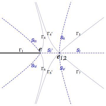
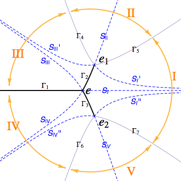
Figure 5: Stokes lines ${\rm Im}\,\Omega=0$ (blue-dashed lines) before (left panel) and after (right panel) transition. Stokes -level lines are black solid lines. Before the transition four Stokes lines emanate from the double point. Stokes phenomena occurs only on $\Gamma_{1}$ representing the fluid boundary. After the transition the double point splits into two branch points, each emanating three Stokes lines. Stokes phenomena occur on shocks $\Gamma_{3},\Gamma_{2}$ where the Painlevé -wave-function accumulates zeros.

6.1 Stokes coefficients

In further analysis, Stokes level-lines (also called anti-Stokes lines), Stokes lines play an important role. They have been already discussed in Sec.58. We recall the major facts.

Stokes level-lines are curved lines determined by the condition ${\rm Re}\,\Omega(X)=0$. On these lines the basis WKB-functions oscillate. There are seven level lines as indicated on the right panel in Fig. 5. Three of them ($\Gamma_{1,2,3}$) are distinct: ${\rm Re}\,\Omega$ approaching to these lines stays positive on both sides. On other lines ${\rm Re}\,\Omega$, changes sign. Being positive in the sector bounded by $\Gamma_{7,3,2,5}$), ${\rm Re}\,\Omega$ becomes negative in adjacent sectors bounded by $\Gamma_{5,4}$ and in the sector bounded by $\Gamma_{6,7}$, and positive again in the sectors bounded by $\Gamma_{4,2,1}$) and $\Gamma_{1,3,6}$).

Stokes lines are the lines where ${\rm Im}\,\Omega(X)=\mbox{const.}$ and connected to a branch point. There are nine of them as shown in the right panel of Fig. 5. All Stokes lines end at infinity.

The semiclassical wave-function is analytic between adjacent Stokes lines separated by a Stokes level line, but may be discontinuous passing through a Stokes line.

Condition (38) requires that at large $X$ the semiclassical approximation suffers a discontinuity only at a fluid boundary $\mbox{Arg}\,X=\pi$ where the wave-function rises as $|X|\to\infty$. This means that on the both sides of the fluid boundary the wave-function possesses a component $\psi_{+}^{WKB}$ which happens to be dominant in the sectors bounded by $\Gamma_{1},\Gamma 4$ and $\Gamma_{1},\Gamma_{6}$. In other words $A_{+}\neq 0$ in these sectors. We set it to be 1. Passing the Stokes-level line $\Gamma_{4}$ the component $\psi_{+}$ becomes recessive. Therefore $A_{-}=0$ to the right of $\Gamma_{4}$, and thus holds everywhere in the sector bounded by $S_{\rm I}^{\prime}$ and $S_{\rm III^{\prime}}$. The symmetry with respect to complex conjugation insures that $A_{-}=0$ also in the sector bounded by $S_{IV^{\prime}}$ and $S_{I^{\prime\prime}}$. Thus

$$\Psi\approx\psi_{+}^{WKB}\,\,\mbox{between $S_{\rm IV^{\prime}}-S_{\rm I^{\prime\prime}}$ and $S_{\rm I^{\prime}}-\,S_{\rm III^{\prime}}$}.$$ (67)

In the sectors adjacent to $\Gamma_{1},\Gamma_{2},\Gamma_{3}$ the WKB approximation of $\psi_{+}^{WKB}$ is dominant. There is no information so far about $A_{-}$ there. Monodromy property of WKB functions determines this coefficient.

Passing through the Stokes-level $\Gamma_{1}$, the term $A_{-}\psi_{-}^{WKB}$ becomes dominant. With a help of (58) we evaluate it at a remote point $X_{1}=|X_{1}|e^{{{i}}(\pi+\delta)},\;|X_{1}|\to\infty$ on the lower side of the $\Gamma_{1}$ ($\delta>0$). We have $-{{i}}A_{-}\psi_{+}({{i}}|X_{1}|e^{{{i}}(-\pi+\delta)})$. But the coefficient of the dominant term is always 1. Thus $A_{-}=i$ in a sector between $\Gamma_{1}$ and $S_{\rm III}$.

Similar arguments determine the Stokes multipliers between Stokes lines $S_{\rm III},\,S_{\rm III^{\prime}}$ and $S_{\rm I},\,S_{\rm I^{\prime}}$. Summing up

$$\Psi=\left\{\begin{array}[]{lr}\psi_{+}^{WKB}+i\psi_{-}^{WKB},\,\mbox{between $\Gamma_{1},\,S_{\rm III}$},\\ \psi_{+}^{WKB}-{{i}}e^{{{i}}\bar{\Phi}}\psi_{-}^{WKB},\,\mbox{between $S_{\rm III^{\prime}},\,S_{\rm III}$},\\ \psi_{+}^{WKB}+{{i}}e^{{{i}}\bar{\Phi}}\psi_{-}^{WKB},\,\mbox{between $S_{\rm I^{\prime}},\,S_{\rm I}$},\\ \psi_{+}^{WKB},\,\mbox{between $S_{\rm I^{\prime}},\,S_{\rm III^{\prime}}$}.\end{array}\right.$$ (68)

The WKB-approximation of the physical wave function in sectors in the lower half plane is achieved by complex conjugation. A special feature of this solution is that at infinity, everywhere in a fluid (a complex plane cut by $\Gamma_{1}$) $\Psi\approx\psi^{WKB}_{+}$ and Eq. (38) holds.

Situation is different at $T<0$. Configuration of Stokes lines and Stokes-level lines is depicted in the left panel of Fig. 5. In this case the only Stokes-level line where $\Re\Omega$ stays positive on both sides is $\Gamma_{1}$. Similar analysis yields a very different result

$$\Psi=\left\{\begin{array}[]{lr}\psi_{+}^{WKB}+i\psi_{-}^{WKB},\,\mbox{between $\Gamma_{1},\,S_{\rm III^{\prime}}$},\\ \psi_{+}^{WKB},\,\mbox{elsewhere\, in\, the\, upper\, half\, plane}.\end{array}\right.$$

7 Semiclassical wave-function and the Hele-Shaw flow

7.1 Darcy Law as an average over the period

The Darcy law follows from the semiclassical wave-function. As it has been described in Sec. 3.2 one recovers the hydrodynamics by averaging oscillating quantities over the period. Let us see how does the wave-function change over the time period $2(\omega+\bar{\omega})$.

Away from sectors adjacent to $\Gamma_{2},\,\Gamma_{3}$ and a fluid boundary $\Gamma_{1}$ the WKB wave-function is equal to $\psi_{+}^{WKB}$. Let us compute an average $\hbar\log\Psi$ over fast oscillations.

First we notice that the term placed in (57) outside of the brackets $\frac{\sigma(\tau+\lambda)}{\sigma(\lambda)\sigma(\tau)}e^{-\zeta(\tau)\lambda}$ is time-periodic. The only change over the period comes from the slowly varying part $Y^{-1/2}e^{\frac{1}{\hbar}\Omega}$ in (57). Thus the leading contribution into $\hbar\log\Psi$ is $\Omega$. Eqs. (36) recover the weak solution of the Hele-Shaw problem.

7.2 Locus of zeroes of the physical wave function and shocks

Physical wave-function oscillates on Stokes level lines. Three Stokes level lines $\Gamma_{1,2,3}$ are special. There, the oscillating WKB wave function possesses two oscillatory terms (68), and, therefore, has zeroes. Position of zeroes $X_{k}$ on these level lines is determined by Bohr-Sommerfeld conditions

$$\Omega_{\hbar}(X_{k})=\left\{\begin{array}[]{lr}{{i}}\hbar\pi(k-\frac{1}{4}),\quad X_{k}\in\Gamma_{1},\\ {{i}}\hbar(k\pi+\frac{\pi}{4}+\frac{1}{2}\overline{\Phi}),\quad X_{k}\in\Gamma_{2},\\ {{i}}\hbar(k\pi+\frac{\pi}{4}-\frac{1}{2}\Phi),\quad X_{k}\in\Gamma_{3},\end{array}\right.$$ (69)

where we evaluate $\Omega_{\hbar}$ from the above of the cuts. We observe a simple pattern selecting the locus of zeros. These are the lines on which ${\rm Re}\,\Omega$ vanishes being positive at both sides as in (32).

Crossing these lines the continuous wave-function experiences an abrupt change on a scale vanishing at $\hbar\to 0$. In that limit the wave-function suffers a discontinuity. The height function, potential, etc., (36) obtained by differentiation of the wave-function follow suit. In the hydrodynamic limit $\hbar\to 0$ the lines of accumulating zeros in the fluid appear as viscous shocks, each zero appear as micro-vortex as has been discussed in (Sec.2.4.1).

8 Discussion and conclusions

We have demonstrated that viscous shocks in singular Hele-Shaw flow are intimately related to non-linear Stokes phenomena of Painlevé I - equation. Stokes-level lines in a complex plane accumulating zeros of the Painlevé -wave-functions evolve as viscous shocks.

Hydrodynamics quantities have a transparent interpretation in terms of evolution of semiclassical approximation of the physical Painlevé - function. In particular, each zero of the holomorphic Painlevé -wave-function is understood as a vortex in the fluid.

Semiclassical approximation of Painlevé -wave-function at $T>0$ features fast time oscillations and also fast spatial oscillations along shocks. Hydrodynamics can be read from these objects either through averaging them over periods of oscillations (36), or, alternatively, by considering discrete moments of time (48) corresponding to half-period where $u_{t}=0$. This sequence of times depends on monodromy data, while hydrodynamics does not

$$\begin{array}[]{lll}T_{n}&=&\left(\frac{5\hbar}{12}\right)^{4/5}\Big{(}(n+{\rm Re}\,\Phi){\rm Re}\,\omega(1)-{\rm Im}\,\Phi\,{\rm Im}\,\omega(1)\Big{)}^{4/5}\\ &\approx&\left(\frac{5\hbar}{12}\cdot 0.7427\right)^{4/5}\left(n+{\rm Re}\,\Phi-{\rm Im}\,\Phi\cdot 0.8173\right)^{4/5}.\end{array}$$

Here $n$ is large positive integer. At these moments the wave-function reads

$$|\Psi^{WKB}(X)|^{2}\sim\left[\frac{X-e(T)}{X^{2}+e(T)X+\frac{g_{3}}{4e(T)}}\right]^{\frac{1}{4}}e^{\frac{4}{5\hbar}{\rm Im}\,(XY-2T\phi(X))}$$

where

$$Y(X)=\sqrt{-4X^{3}+12TX+g_{3}},$$

$$\phi(X)=6\int_{e(T)}^{X}\left(X^{\prime}+\frac{g_{3}}{8T}\right)\frac{dX^{\prime}}{Y(X^{\prime})}.$$

The numerical value of $g_{3}$ and $e(T)$ are given in (28) and (30) respectively by

$$g_{3}\approx-7.321762\,T^{3/2},\quad e(T)\approx-0.553594\sqrt{T}.$$

Eqs. (36) yields hydrodynamics results for potential and velocity of the flow supplemented by semiclassical corrections.

Discrete nature of time and discrete structure of shocks supports a “corpuscular” interpretation of singular flow. One may associate a space between zeros in a shock line with a particle aggregating on a shock. A particle arrives to a shock every time interval equal to $\hbar^{4/5}$.

Finally we comment that the present analysis does not discriminates within a one-parametric family of physical solutions characterized by the Bloch factor $\Phi$. We conjecture that a unique solution will be selected by the requirement that Painlevé -function is associated with some stochastic process. This requirement may select $\Phi$. An interesting candidate is ${\rm Im}\,\Phi=0$. Then the Bloch factor is a pure phase. According to (47) $\Phi=\pi/6$ and $|C|=\sqrt{3}/{2}$.

References

References

- [1] S.-Y. Lee, R. Teodorescu and P. Wiegmann. Shocks and finite-time singularities in Hele-Shaw flow. Phys. D, 238(14):1113–1128, 2009.
- [2] S-Y. Lee, R. Teodorescu and P. Wiegmann. Weak solution of the Hele-Shaw problem: shocks and viscous fingering, arXiv:0812.0579v1 [cond-mat.soft], 2008.
- [3] Y. Couder. Perspectives in Fluid Dynamics. Cambridge Univ. Press, 2000.
-
[4]
T. A. Witten and L. M. Sander.
Diffusion-limited aggregation, a kinetic critical phenomenon.
Phys. Rev. Lett., 47(19):1400–1403, 1981;
M. B. Hastings and L. S. Levitov. Laplacian growth as one-dimensional turbulence. Physica D, 116:244, 1998;
J. Mathiesen, I. Procaccia, H. L. Swinney and M. Thrasher. The universality class of diffusion-limited aggregation and viscous fingering. Europhysics Letters, 76(2): 257, 2006; - [5] B. Shraiman and D. Bensimon. Singularities in nonlocal interface dynamics. Phys. Rev. A, 30(5):2840–2842, 1984.
- [6] S. D. Howison, J. R. Ockendon, and A. A. Lacey. Singularity development in moving-boundary problems. Quart. J. Mech. Appl. Math., 38(3):343–360, 1985.
- [7] Y. E. Hohlov and S. D. Howison. On the classification of solutions to the zero-surface-tension model for Hele-Shaw free boundary flows. Quart. Appl. Math., 51(4):777–789, 1993.
- [8] R. Teodorescu, P. Wiegmann, and A. Zabrodin. Unstable fingering patterns of Hele-Shaw flows as a dispersionless limit of the KdV hierarchy. Phys.Rev.Lett. 95:044502, 2005.
- [9] L. C. Evans. Partial differential equations, volume 19 of Graduate Studies in Mathematics. American Mathematical Society, Providence, RI, 1998.
- [10] G. B. Whitham. Linear and nonlinear waves. Pure and Applied Mathematics (New York). John Wiley & Sons Inc., New York, 1999.
- [11] B. A. Dubrovin and S. P. Novikov. Hydrodynamics of weakly deformed soliton lattices. Differential geometry and Hamiltonian theory. Uspekhi Mat. Nauk, 44(6(270)):29–98, 203, 1989.
- [12] I. M. Krichever. The -function of the universal Whitham hierarchy, matrix models and topological field theories. Comm. Pure Appl. Math., 47(4):437–475, 1994.
- [13] F. Fucito, A. Gamba, M. Martellini, and O. Ragnisco. Non-linear WKB analysis of the string equation. International Journal of Modern Physics B, 6:2123, 1992.
- [14] P. G. Grinevich and S. P. Novikov. String equation. II. Physical solution. Algebra i Analiz, 6(3):118–140, 1994.
- [15] I. Krichever, M. Mineev-Weinstein, P. Wiegmann, and A. Zabrodin. Laplacian growth and Whitham equations of soliton theory. Physica D, 198(1-2):1–28, 2004.
- [16] M. Jimbo and T. Miwa. Deformation of linear ordinary differential equations. I, II. Proc. Japan Acad. Ser. A Math. Sci., 56(4):143–148, 149–153, 1980.
- [17] A. A. Kapaev. Monodromy deformation approach to the scaling limit of the Painlevé first equation. Differentsialnya Uravneniya, 24:1684, 1988.
- [18] Y. Takei. On the connection formula for the first Painlevé equation from the viewpoint of the exact WKB analysis Surikaisekikenkyusho Kokyuroku 931: 70-99, 1995
- [19] A. A. Kapaev. Monodromy deformation approach to the scaling limit of the Painlevé first equation. In The Kowalevski property (Leeds, 2000), volume 32 of CRM Proc. Lecture Notes, pages 157–179. Amer. Math. Soc., Providence, RI, 2002.
- [20] A. A. Kapaev. Quasi-linear stokes phenomenon for the Painlevé first equation. J. Phys. A, 37(46):11149–11167, 2004.
- [21] A. S. Fokas, A. R. Its, A. A. Kapaev, V. Yu. Novokshenov. Painlevé Transcendents: The Riemann-Hilbert Approach. American Mathematical Society, 2006.
- [22] O. Agam, E. Bettelheim, P. Wiegmann, A. Zabrodin. Viscous fingering and a shape of an electronic droplet in the Quantum Hall regime. Phys.Rev.Lett. 88:236801, 2002.
- [23] R. Teodorescu, E. Bettelheim, O. Agam, A. Zabrodin, and P. Wiegmann. Normal random matrix ensemble as a growth problem. Nuclear Physics B, 704:407, 2005.
- [24] R. Teodorescu. Generic critical points of normal matrix ensembles. J. Phys. A: Math. Gen. 39: 8921 - 8932, 2006.
- [25] F. David. Phases of the large- matrix model and nonperturbative effects in D gravity. Nuclear Phys. B, 348(3):507–524, 1991.
-
[26]
A. S. Fokas., A. R. Its and A. V. Kitaev.
Discrete Painlevé equations and their appearance in quantum gravity. Comm. Math. Phys. 142: 313-44, 1991;
The isomonodromy approach to matrix models in 2D quantum gravity. Comm. Math. Phys. 147: 395-430, 1992. - [27] M. Duits and A. B. J. Kuijlaars. Painlevé I asymptotics for orthogonal polynomials with respect to a varying quartic weight. Nonlinearity, 19(10):2211–2245, 2006.
- [28] Yu. E. Hohlov, S.D. Howison, C. Huntingford, J. R. Ockendon and A. A.Lacey. Model for non- smooth free boundaries in Hele-Shaw flows. Q. J. Mech. Appl. Math. 47 (1), 107-128 (1994).
- [29] A. A. Lacey, S. D. Howison, J. R. Ockendon and P. Wilmott. Irregular morphologies in unstable Hele-Shaw free boundary problems. Q. J. Mech. Appl. Math. 43 (3), 387-405 (1990).
- [30] H. Flaschka, M. G. Forest, and D. W. McLaughlin. Multiphase averaging and the inverse spectral solution of the Korteweg-de Vries equation. Comm. Pure Appl. Math., 33(6):739–784, 1980.
- [31] L. A. Galin. Unsteady filtration with a free surface. Dokl. Akad. Nauk SSSR 47: 250-253, 1945 (In Russian); English transl., (Dokl.) Acad. Sci. URSS, 47: 246-249, 1945.
- [32] P. Ya. Polubarinova-Kochina. On a problem of the motion of the contour of a petroleum shell. Dokl. Akad. Nauk USSR, 47 no. 4: 254-257, 1945 (in Russian); English transl., On the displacement of the oil-bearing contour, C. R. (Dokl.) Acad. Sci. URSS, 47: 250-254, 1945.
- [33] P. Di Francesco, P. Ginsparg, and J. Zinn-Justin. 2D Gravity and Random Matrices. Phys. Rep., 254:1–133, 1995.
- [34] M. Bertola. Boutroux curves with external field: equilibrium measures without a minimization problem. arxiv.org/list/nlin.SI/0705.3062.
- [35] P. Boutroux. Recherches sur les transcendantes de M. Painlevé et l’étude asymptotique des équations différentielles du second ordre. Ann. Sci. École Norm. Sup. (3), 30:255–375, 1913.
- [36] I. M. Krichever Method of averaging for two-dimensional integrable equations. Funct. Anal. Appl. 22: 200-13, 1988.
- [37] Kapaev A. A., Kitaev A. V. Connection formulae for the first Painlevé transcendent in the complex domain. Lett. Math. Phys. 27, 243-52, 1993.
- [38] P. Holmes and D. Spence. On a Painlevé-type boundary value problem. Quart. J. Mech. Appl. Math., 37(4):525–538, 1984.
- [39] E. Witten. Two dimensional gravity and intersection theory on moduli space. Surveys In Diff. Geom. 1: 243, 1991.
- [40] N. Joshi and A. V. Kitaev. On Boutroux Tritronqueé Solutions of the First Painlevé Equation. Studies in Applied Mathematics 107: 253-291, 2001.
- [41] R. Garnier. Étude de l’intégrale générale de l’équation VI de M. Painlevé dans le voisinage de ses singularités transcendantes. Ann. Sci. École Norm. Sup. (3), 34:239–353, 1917.
- [42] W. Wasow. Linear turning point theory, volume 54 of Applied Mathematical Sciences. Springer-Verlag, New York, 1985.