Dimensional recurrence relations:
an easy way to evaluate higher orders of expansion in $\ep$

Abstract

Applications of a method recently suggested by one of the authors (R.L.) are presented. This method is based on the use of dimensional recurrence relations and analytic properties of Feynman integrals as functions of the parameter of dimensional regularization, $d$. The method was used to obtain analytical expressions for two missing constants in the $\ep$-expansion of the most complicated master integrals contributing to the three-loop massless quark and gluon form factors and thereby present the form factors in a completely analytic form. To illustrate its power we present, at transcendentality weight seven, the next order of the $\ep$-expansion of one of the corresponding most complicated master integrals. As a further application, we present three previously unknown terms of the expansion in $\ep$ of the three-loop non-planar massless propagator diagram. Only multiple $\zeta$ values at integer points are present in our result.

1 Introduction

Quite recently a new method [1] of evaluating Feynman integrals was suggested. It is based on the use of dimensional recurrence relations [2] and analytic properties of Feynman integrals as functions of the parameter of dimensional regularization, $d$. Here we are going to describe new results of its application. In the next section we give a summary of the evaluation of the two previously analytically unknown coefficients of transcendentality weight six in the $\ep$-expansion of two master integrals contributing to the three-loop massless form factors [3]. We also present, at transcendentality weight seven, the next order of the $\ep$-expansion of one of the corresponding most complicated master integrals. In Section 3, we report on the evaluation of higher orders of expansion in $\ep$ of the three-loop non-planar massless propagator diagram and, in Section 4, we discuss our results.

2 Evaluating master integrals for
three-loop form factors

The integration-by-part reduction reduces the problem to the calculation of a small number of master integrals. All the master integrals apart from three most complicated master integrals contributing to the three-loop massless form factors have been analytically evaluated in [4, 5]. About one year ago, one of the three most complicated master integrals (called $A_{9,1}$ in [4, 5, 6, 7]) and the pole parts of $A_{9,4}$ and $A_{9,2}$ shown in Figs. 1 and 2

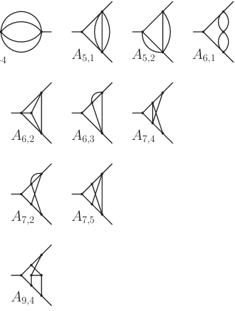
Figure 1: Master integrals for $A_{9,4}$.

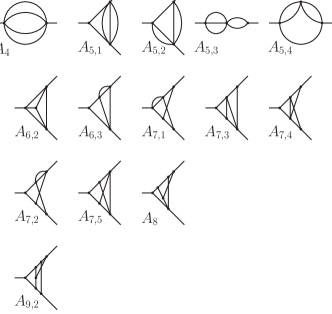
Figure 2: Master integrals for $A_{9,2}$.

were evaluated analytically, while the $\ep^{0}$ parts of $A_{9,4}$ and $A_{9,2}$ were evaluated numerically — see [6, 7].

In [3], the two missing ingredients, i.e. the finite parts of $A_{9,4}$ and $A_{9,2}$, were evaluated analytically. According to the method of [1] it is necessary, before evaluating $A_{9,4}$ and $A_{9,2}$, to know all lower master integrals. They are shown in the same figures. Four rows of diagrams in each figure correspond to complexity levels 0, 1, 2 and 3. Details of the calculation can be found in [1]. Here are the corresponding results:

$$A_{9,4}(4-2\ep)={\rm e}^{-3\gamma_{E}\ep}\biggl{\{}-\frac{1}{9\ep^{6}}-\frac{8}{9\ep^{5}}$$

$$+\left[1+\frac{43\pi^{2}}{108}\right]\frac{1}{\ep^{4}}+\left[\frac{109\zeta(3)}{9}+\frac{14}{9}+\frac{53\pi^{2}}{27}\right]\frac{1}{\ep^{3}}$$

$$+\left[\frac{608\zeta(3)}{9}-17-\frac{311\pi^{2}}{108}-\frac{481\pi^{4}}{12960}\right]\frac{1}{\ep^{2}}$$

$$+\left[-\frac{949\zeta(3)}{9}-\frac{2975\pi^{2}\zeta(3)}{108}+\frac{3463\zeta(5)}{45}\right.$$

$$\left.+84+\frac{11\pi^{2}}{18}+\frac{85\pi^{4}}{108}\right]\frac{1}{\ep}$$

$$+\left[\frac{434\zeta(3)}{9}-\frac{299\pi^{2}\zeta(3)}{3}-\frac{3115\zeta(3)^{2}}{6}+\frac{7868\zeta(5)}{15}\right.$$

$$\left.-339+\frac{77\pi^{2}}{4}-\frac{2539\pi^{4}}{2592}-\frac{247613\pi^{6}}{466560}\right]+O(\ep)\biggr{\}}\;;$$

$$A_{9,2}(4-2\ep)={\rm e}^{-3\gamma_{E}\ep}\biggl{\{}-\frac{2}{9\ep^{6}}-\frac{5}{6\ep^{5}}$$

$$+\left[\frac{20}{9}+\frac{17\pi^{2}}{54}\right]\frac{1}{\ep^{4}}$$

$$+\left[\frac{31\zeta(3)}{3}-\frac{50}{9}+\frac{181\pi^{2}}{216}\right]\frac{1}{\ep^{3}}$$

$$+\left[\frac{347\zeta(3)}{18}+\frac{110}{9}-\frac{17\pi^{2}}{9}+\frac{119\pi^{4}}{432}\right]\frac{1}{\ep^{2}}$$

$$+\left[-\frac{514\zeta(3)}{9}-\frac{341\pi^{2}\zeta(3)}{36}+\frac{2507\zeta(5)}{15}\right.$$

$$\left.-\frac{170}{9}+\frac{19\pi^{2}}{6}+\frac{163\pi^{4}}{960}\right]\frac{1}{\ep}$$

$$+\left[\frac{1516\zeta(3)}{9}-\frac{737\pi^{2}\zeta(3)}{24}-29\zeta(3)^{2}+\frac{2783\zeta(5)}{6}\right.$$

$$\left.-\frac{130}{9}+\frac{\pi^{2}}{2}-\frac{943\pi^{4}}{1080}+\frac{195551\pi^{6}}{544320}\right]+O(\ep)\biggr{\}}\;.$$

An independent calculation of the form factors was performed quite recently [8] and the agreement with the previous results was established. Motivated by a future four-loop calculation the authors calculated also the subleading $O(\ep)$ terms for the fermion-loop type contributions. We think that the analytic calculation of the whole $O(\ep)$ part of the form factors is feasible at the moment. To illustrate this possibility we have calculated the $O(\ep^{2})$ order of the $\ep$-expansion of one of the corresponding most complicated master integrals, $A_{9,1}$, which is of transcendentality weight seven:

$$A_{9,1}(4-2\ep)=e^{-3\gamma_{E}\ep}\biggl{\{}\frac{1}{18\ep^{5}}-\frac{1}{2\ep^{4}}$$

$$+\frac{1}{\ep^{3}}\left(\frac{53}{18}+\frac{29\pi^{2}}{216}\right)$$

$$+\frac{1}{\ep^{2}}\left(\frac{35\zeta(3)}{18}-\frac{29}{2}-\frac{149\pi^{2}}{216}\right)$$

$$+\frac{1}{\ep}\left(-\frac{307\zeta(3)}{18}+\frac{129}{2}+\frac{139\pi^{2}}{72}+\frac{5473\pi^{4}}{25920}\right)$$

$$+\left(\frac{793\zeta(5)}{10}+\frac{871\pi^{2}\zeta(3)}{216}+\frac{1153\zeta(3)}{18}\right.$$

$$\left.-\frac{3125\pi^{4}}{5184}-\frac{19\pi^{2}}{8}-\frac{537}{2}\right)$$

$$+\ep\left(-\frac{287\zeta(3)}{2}+\frac{2969\pi^{2}\zeta(3)}{216}+\frac{5521\zeta(3)^{2}}{36}\right.$$

$$\left.-\frac{8251\zeta(5)}{30}+\frac{2133}{2}-\frac{97\pi^{2}}{8}\right.$$

$$\left.+\frac{4717\pi^{4}}{28115}+\frac{761151\pi^{6}}{186624}\right)$$

$$+\ep^{2}\left(\frac{195\zeta(3)}{2}-\frac{5887\pi^{2}\zeta(3)}{72}+\frac{138403\pi^{4}\zeta(3)}{25920}\right.$$

$$\left.+\frac{799\zeta(3)^{2}}{4}+\frac{22487\zeta(5)}{30}-\frac{11987\pi^{2}\zeta(5)}{10115}\right.$$

$$\left.+\frac{228799\zeta(7)}{126}-\frac{8181}{2}+\frac{969\pi^{2}}{8}\right.$$

$$\left.-\frac{1333\pi^{4}}{320}-\frac{4286603\pi^{6}}{6531840}\right)+\ldots\biggr{\}}\;.$$

3 Non-planar massless propagator diagram

It is also natural to try to apply the same method to evaluate the three previously analytically unknown coefficients of transcendentality weight six in the $\ep$-expansion of three master integrals contributing to the three-loop static quark potential [9, 10, 11, 12, 13, 14]. These are $I_{11},I_{16},I_{18}$ in Fig. 3.

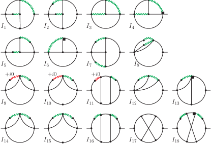
Figure 3: Most complicated master integrals for the three-loop static quark potential.

This work is in progress [15]. Here we would like to present, as a by-product of this activity, new results for one of the master integrals which are lower than $I_{18}$. Let us consider $I_{17}$ which is a master integral for three-loop massless propagator integrals. The famous value $20\zeta(5)$ at $d=4$ is known for a long time [16]. The linear term in the $\ep$-expansion was obtained in [17]. The quadratic term was recently evaluated [18]. To illustrate the power of the present method we have evaluated the three next terms so that we have a result up to $\ep^{5}$.

The diagram itself and the corresponding four lower diagrams are shown in Fig. 4

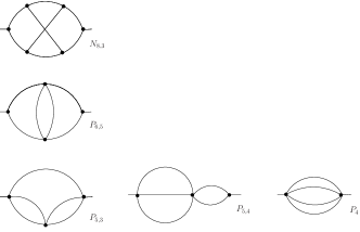
Figure 4: Master integrals for $I_{17}$.

The labelling for $I_{17}\equiv N_{8,3}$ and its lower master integrals is taken from the future publication [15]. This master integral itself has complexity level 2, the master integral $P_{6,5}$ has complexity level 1, while the other three master integrals can be expressed in terms of gamma functions at general $d$.

The lowering recurrence relation for this integral provides the following expression of $N_{8,3}^{(d+2)}$ in terms of master integrals in $d$ dimensions:

$$N_{8,3}^{(d+2)}=\frac{(d-4)}{8(d-2)(d-1)(2d-7)(2d-5)}N_{8,3}^{(d)}$$

$$+\frac{4\left(5d^{2}-28d+38\right)}{(d-4)^{2}(d-2)(d-1)(2d-5)}P_{5,3}^{(d)}$$

$$+\left[4(d-4)(d-2)(d-1)(2d-7)(2d-5)\right]^{-1}$$

$$\times(3d-8)^{-1}\left(37d^{3}-313d^{2}+858d-752\right)P_{6,5}^{(d)}$$

$$-\left(43d^{4}-478d^{3}+1963d^{2}-3530d+2352\right)$$

$$\times\left[2(d-4)^{2}(d-3)(d-2)(d-1)\right]^{-1}$$

$$\times\left[(2d-7)(2d-5)\right]^{-1}P_{5,4}^{(d)}$$

$$-\left[(d-4)^{3}(d-3)^{2}(d-2)\right]^{-1}$$

$$\times\left[(d-1)(2d-7)(3d-8)\right]^{-1}$$

$$\times\left(401d^{6}-7251d^{5}+54491d^{4}-217784d^{3}\right.$$

$$\left.+486264d^{2}-581248d+287232\right)P_{4}^{(d)}\;.$$

We obtain the following result to order $\ep^{5}$:

$$I_{17}=\frac{{\rm e}^{-3\gamma_{E}\ep}}{1-2\ep}\biggl{\{}20\zeta(5)+\ep\left(68\zeta(3)^{2}+\frac{10\pi^{6}}{189}\right)$$

$$+\ep^{2}\left(\frac{34\pi^{4}\zeta(3)}{15}-5\pi^{2}\zeta(5)+450\zeta(7)\right)$$

$$+\ep^{3}\left(-\frac{9072}{5}\zeta(5,3)-2588\zeta(3)\zeta(5)\right.$$

$$\left.-17\pi^{2}\zeta(3)^{2}+\frac{6487\pi^{8}}{10500}\right)$$

$$+\ep^{4}\left(-\frac{4897\pi^{6}\zeta(3)}{630}-\frac{6068\zeta(3)^{3}}{3}+\frac{13063\pi^{4}\zeta(5)}{120}\right.$$

$$\left.-\frac{225\pi^{2}\zeta(7)}{2}+\frac{88036\zeta(9)}{9}\right)$$

$$+\ep^{5}\left(\frac{2268}{5}\pi^{2}\zeta(5,3)+42513\zeta(8,2)\right.$$

$$\left.-145328\zeta(3)\zeta(7)-73394\zeta(5)^{2}+647\pi^{2}\zeta(3)\zeta(5)\right.$$

$$\left.-\frac{11813\pi^{4}\zeta(3)^{2}}{120}+\frac{28138577\pi^{10}}{9355500}\right)+\ldots\biggr{\}}\;,$$

where $\zeta(n,m)$ are multiple zeta values (see, e.g., [19]). Observe that the pulling out the standard prefactor $1/(1-2\ep)$ in results for massless propagator integrals (see, e.g., [16, 17, 20]) provides the homogeneous transcendentality weight in all the orders of the expansion in $\ep$. We see this property in our new piece of the result, i.e. in the $\ep^{i}$ terms with $i=3,4,5$. Let us emphasize that this property is very useful when using PSLQ [21] because the number of constants that can be present in a result is essentially reduced. In fact, we indeed arrived at the above result using PSLQ but could here proceed even without the homogeneous transcendentality weight because, within the method of [1], we obtained, for $I_{17}$, a very well convergent double series so that we could obtain the accuracy of thousand of digits or more. For the same reason, we can obtain higher terms of the expansion in $\ep$, i.e., $\ep^{6}$ etc.

If one pulls out a more sophisticated prefactor [16, 20] (see the next equation) the pure $\pi^{2}$ factors will not be present in the result. We see that this property is satisfied indeed:

$$I_{17}=(1-2\ep)^{2}\left(\frac{\Gamma(1-\ep)^{2}\Gamma(1+\ep)}{\Gamma(2-2\ep)}\right)^{3}\biggl{\{}20\zeta(5)$$

$$+\ep\left(68\zeta(3)^{2}+\frac{10\pi^{6}}{189}\right)$$

$$+\ep^{2}\left(\frac{34\pi^{4}\zeta(3)}{15}+450\zeta(7)\right)$$

$$+\ep^{3}\left(-\frac{9072}{5}\zeta(5,3)-2448\zeta(3)\zeta(5)+\frac{8519\pi^{8}}{13500}\right)$$

$$+\ep^{4}\left(-\frac{1292\pi^{6}\zeta(3)}{189}-\frac{4640\zeta(3)^{3}}{3}\right.$$

$$\left.+\frac{552\pi^{4}\zeta(5)}{5}+\frac{88036\zeta(9)}{9}\right)$$

$$+\ep^{5}\left(42513\zeta(8,2)-142178\zeta(3)\zeta(7)-73022\zeta(5)^{2}\right.$$

$$\left.-\frac{232\pi^{4}\zeta(3)^{2}}{3}+\frac{593053\pi^{10}}{187110}\right)+\ldots\biggr{\}}\;.$$

Let us observe that in [22] it was proven that the coefficients in the $\ep$-expansion of planar massless propagator diagrams up to five loops should be expressed in terms of multiple zeta values, while the non-planar graphs may contain, in addition, multiple sums with 6th roots of unity. However, in the above result, only multiple zeta values are present.

4 Conclusion

Let us emphasize that in the present paper we used method of Ref.[1] in combination with several other methods. We already mentioned PSLQ. Then, as it was explained in [1, 3], it is implied that the IBP reduction is solved for a given problem so that one can obtain dimensional recurrence relations. To do this we used the code called FIRE [24] and the code based on [25] but, of course, one can use other methods. Moreover, we use a sector decomposition [26, 27, 28] implemented in the code FIESTA [28, 29] to determine the position and the order of the poles in the basic stripe. To fix remaining constants in the homogenous solution of dimension recurrence relations we apply the method of Mellin–Barnes representation [30, 31, 32].

The method used in the present calculations looks quite promising and we expect it to be applied not only in the problems discussed above but also in many other situations.

Acknowledgements. We would like to thank D.J. Broadhurst and K.G. Chetyrkin for stimulating discussions. This work was supported by the Russian Foundation for Basic Research through grant 08–02–01451. V.S. appreciates the financial support of KIT through project SFB/TR 9 for the participation in the workshop.

References

- [1] R. N. Lee, Nucl. Phys. B 830 (2010) 474 [arXiv:0911.0252 [hep-ph]].
- [2] O. V. Tarasov, Phys. Rev. D 54 (1996) 6479.
- [3] R. N. Lee, A. V. Smirnov and V. A. Smirnov, arXiv:1001.2887 [hep-ph].
- [4] T. Gehrmann, G. Heinrich, T. Huber and C. Studerus, Phys. Lett. B 640, 252 (2006) [hep-ph/0607185].
- [5] G. Heinrich, T. Huber and D. Maître, Phys. Lett. B 662 (2008) 344 [arXiv:0711.3590 [hep-ph]].
- [6] P. A. Baikov, K. G. Chetyrkin, A. V. Smirnov, V. A. Smirnov and M. Steinhauser, Phys. Rev. Lett. 102 (2009) 212002 [arXiv:0902.3519 [hep-ph]].
- [7] G. Heinrich, T. Huber, D. A. Kosower and V. A. Smirnov, Phys. Lett. B 678 (2009) 359 [arXiv:0902.3512 [hep-ph]].
- [8] T. Gehrmann, E. W. N. Glover, T. Huber, N. Ikizlerli and C. Studerus, arXiv:1004.3653 [hep-ph].
- [9] A. V. Smirnov, V. A. Smirnov and M. Steinhauser, PoS RADCOR2007 (2007) 024.
- [10] A. V. Smirnov, V. A. Smirnov and M. Steinhauser, Phys. Lett. B 668 (2008) 293 [arXiv:0809.1927 [hep-ph]].
- [11] A. V. Smirnov, V. A. Smirnov and M. Steinhauser, Nucl. Phys. Proc. Suppl. 183 (2008) 308 [arXiv:0807.0365 [hep-ph]].
- [12] A. V. Smirnov, V. A. Smirnov and M. Steinhauser, Phys. Rev. Lett. 104 (2010) 112002 [arXiv:0911.4742 [hep-ph]].
- [13] C. Anzai, Y. Kiyo and Y. Sumino, Phys. Rev. Lett. 104, 112003 (2010) [arXiv:0911.4335 [hep-ph]].
- [14] A. V. Smirnov, V. A. Smirnov and M. Steinhauser, arXiv:1001.2668 [hep-ph].
- [15] R. N. Lee, A. V. Smirnov and V. A. Smirnov, to be published.
- [16] K. G. Chetyrkin, A. L. Kataev and F. V. Tkachov, Nucl. Phys. B 174 (1980) 345.
- [17] D. I. Kazakov, Teor. Mat. Fiz. 58 (1984) 343.
- [18] S. Bekavac, Comput. Phys. Commun. 175 (2006) 180 [arXiv:hep-ph/0505174].
- [19] J. Blumlein, D. J. Broadhurst and J. A. M. Vermaseren, Comput. Phys. Commun. 181 (2010) 582 [arXiv:0907.2557 [math-ph]].
- [20] D. J. Broadhurst, arXiv:hep-th/9909185.
- [21] H.R.P. Ferguson and D.H. Bailey, RNR Technical Report, RNR-91-032; H.R.P. Ferguson, D.H. Bailey and S. Arno, NASA Technical Report, NAS-96-005.
- [22] F. Brown, Commun. Math. Phys. 287, 925 (2009) [arXiv:0804.1660 [math.AG]].
- [23] A. V. Smirnov, V. A. Smirnov and M. Tentyukov, arXiv:0912.0158 [hep-ph].
- [24] A. V. Smirnov, JHEP 0810, 107 (2008) [arXiv:0807.3243 [hep-ph]].
- [25] R. N. Lee, JHEP 0807 (2008) 031 [arXiv:0804.3008 [hep-ph]].
- [26] T. Binoth and G. Heinrich, Nucl. Phys. B, 585 (2000) 741; Nucl. Phys. B, 680 (2004) 375; Nucl. Phys. B, 693 (2004) 134.
- [27] C. Bogner and S. Weinzierl, Comput. Phys. Commun. 178 (2008) 596 [arXiv:0709.4092 [hep-ph]]; Nucl. Phys. Proc. Suppl. 183 (2008) 256 [arXiv:0806.4307 [hep-ph]].
- [28] A. V. Smirnov and M. N. Tentyukov, Comput. Phys. Commun. 180 (2009) 735 [arXiv:0807.4129 [hep-ph]].
- [29] A. V. Smirnov, V. A. Smirnov and M. Tentyukov, arXiv:0912.0158.
-
[30]
V. A. Smirnov, Phys. Lett. B 460 (1999) 397;
J. B. Tausk, Phys. Lett. B 469 (1999) 225;
-
[31]
M. Czakon, Comput. Phys. Commun. 175 (2006) 559;
A. V. Smirnov and V. A. Smirnov, JHEP 05 (2009) 004 [arXiv:0901.0386 [hep-ph]]. -
[32]
V. A. Smirnov, Evaluating Feynman Integrals, Springer Tracts
Mod. Phys. 211 (2004) 1;
V. A. Smirnov, Feynman integral calculus, Berlin, Germany: Springer (2006) 283 p.