A novel subtraction scheme for double-real radiation at NNLO
Abstract
A general subtraction scheme, STRIPPER (SecToR Improved Phase sPacE for real Radiation), is derived for the evaluation of next-to-next-to-leading order (NNLO) QCD contributions from double-real radiation to processes with at least two particles in the final state at leading order. The result is a Laurent expansion in the parameter of dimensional regularization, the coefficients of which should be evaluated by numerical Monte Carlo integration. The two main ideas are a two-level decomposition of the phase space, the second one factorizing the singular limits of amplitudes, and a suitable parameterization of the kinematics allowing for derivation of subtraction and integrated subtraction terms from eikonal factors and splitting functions without non-trivial analytic integration.
1 Introduction
Compared to the number of phenomenological applications, where NNLO QCD corrections are indispensable, the effort put into the construction of general subtraction schemes for real radiation at this level of perturbation theory is astounding. The main problems encountered are either, that the method is not general and requires tedious adaptation to every specific problem, or that there are many highly non-trivial divergent dimensionally regulated integrals to evaluate.
This state of affairs is to be contrasted with the comforting situation at the NLO level, where general solutions have been available for long. The approach of choice is that of Catani and Seymour [1], later extended to massive states [2] and arbitrary polarizations in real radiation [3]. In fact, we would encourage the non-expert reader to consult the original paper [1], since it gives a thorough discussion of all aspects of the problem. The present letter assumes such knowledge.
The main features of the Catani-Seymour subtraction scheme are the smooth interpolation of the subtraction terms between soft and collinear limits and independence from the phase space parameterization achieved by a remapping of phase space points onto the reduced phase space with one parton less. There is another scheme at NLO derived by Kunszt, Frixione and Signer (FKS) [4], which is vastly different on the conceptual side. Here, the phase space is first decomposed into sectors (originally with the help of the jet function; an independent decomposition has been proposed in [5]), and then parameterized with energy and angle variables for easy extraction of the subtraction terms. Precisely these ideas will turn out to be crucial for the scheme that we shall derive.
Many approaches have been proposed at NNLO. The most successful ones are Sector Decomposition [6, 7, 8] and Antenna Subtraction [9]. Sector decomposition is conceptually entirely different from the NLO methods cited above. The idea is to derive a Laurent expansion for the given amplitude, by first ingeniously parameterizing the complete phase space, mapping it onto the unit hypercube, and then dividing it into simplexes, in which singularities are factorized. The parameterization is adapted to different singularity structures for different diagram classes. A detailed description on the particular example of Higgs boson production can be found in [10]. The main drawback is that one has to repeat everything for a new problem, which is relatively easy, if it involves the same number of particles in the final state with the same mass distribution, but is expected to be a major effort otherwise. Antenna subtraction, on the other hand, uses complete matrix elements of simpler processes as building blocks for the subtraction. In this way, the integration over the unresolved particle phase space can be made largely with multi-loop methods. It is this latter part that involves most work, but the result is general and can be applied to other processes without modification. The drawback of this approach is the efficiency loss due to the fact that azimuthal correlations characteristic of collinear limits are not taken into account, as the simplified matrix elements correspond to unpolarized scattering. There are also other methods, which are either specific to a class of problems, such as that of [11], which solves the problem for the production of colorless states, or still require the integration of the subtraction terms, as for example in [12] and [13].
The purpose of this letter is to present a new approach, which should provide a method both general and simple to derive. To this end, we need to specify, which problems are essentially difficult and which are not. Unlike at NLO, there are in fact two different problems involving real radiation at NNLO. One involves the emission of one additional parton (in comparison to leading order) out of virtual diagrams. Usually called single-real radiation, since only one parton can become unresolved, it can be treated by any of the NLO methods. Of course, the subtraction terms require a slight modification. In fact, we believe that the FKS approach will provide the result with the least effort. By this argument, we shall ignore single-real radiation and concentrate on double-real radiation. The latter problem involves two unresolved partons and only tree-level matrix elements. The method presented will not depend on the nature of the initial state. Let us, however, consider the more difficult case of hadronic collisions. Due to the factorization theorem, the result is a convolution of partonic cross sections with Parton Distribution Functions (PDFs). As long as the partonic cross section is an ordinary function, this convolution can be considered independently (see Section 2.1). Indeed, in actual Monte Carlo generators, one first generates the fractions of hadron momenta to be assigned to the partons and then works in the center-of-mass frame of the partons, multiplying every event by the PDF weight only at the end. This is the point of view that we shall adopt as well. To summarize: we will consider the derivation of the Laurent expansion of the double-real radiation contributions for fixed initial parton energies.
The main concept of our approach is to mix some ideas of the FKS NLO subtraction scheme with those of Sector Decomposition. We will decompose the phase space in two stages. At the first stage, we will divide the problem into triple- and double-collinear sectors. Then, using an energy-angle parameterization of the phase space, we will perform an ordinary sector decomposition mimicking the physical singular limits. The crucial novelty is that we will show how to obtain general subtraction terms from the last sector decomposition. Here, we will use the knowledge of NNLO singular behavior of QCD amplitudes as studied in [14, 15, 16] and summarized in [17]. While we will not give explicit expressions for the subtraction terms, a task impossible in a letter due to the multitude of cases, it is easy to rederive them following the description.
In the next section, we will derive the scheme on the example of massive particle production. The reason for this restriction on the final state is that this letter will be followed by a companion publication with process specific information and numerical results for our first application: top quark pair production. A subsequent section will, however, present the generalization to arbitrary final states.
2 Massive final states at leading order
2.1 Phase space
Let us assume that there are only two massless partons in the final state, the other final state particles being massive. In case there is only one massive final state, the presence of soft singularities leads to a cross section, which is a distribution in the partonic center-of-mass energy squared, . We will not take this possibility into account, since it has already been extensively studied for all processes of phenomenological interest and is a special case involving additional complications. The cross section will, therefore, be an ordinary function of . The considered process corresponds to the following kinematical configuration
| (1) |
with
| (2) |
where are -dimensional momentum vectors. The -dimensional phase space can be written as
| (3) |
The above definition suggests a factorization of the phase space for this problem into the three-particle production phase space of the two massless partons together with an object with invariant mass , and a decay phase space of the composite with momentum into the massive particles. Such a factorization is motivated by the fact that most divergences are due to the vanishing of invariants involving only massless states momenta. The divergences not belonging to this class are soft and involve the massive states momenta. In this case, the inverse propagators responsible for the singularities vanish proportionally to a linear combination of the energy components of and . This will force us to use these energy components as part of the phase space parameterization. At this point the phase space can be written as
| (4) | |||||
The integrations over can be performed by exploiting the -function, which leaves
| (5) | |||||
where
| (6) |
The same result could have been obtained directly (and trivially) from the original expression given in Eq. (3), but we wish to keep the interpretation of the integral as described above. Notice that the parameterization of will be of no further concern to us, apart from the fact that it is a continuous function of . Let us mention, however, that a particularly suitable approach is to define in the center-of-mass frame of . In this case, suitable integration parameters can be chosen to allow the integration over to be the first in Eq. (5).
At this point, we can already derive the boundaries of the three-particle phase space. From here on, we will work in the center-of-mass system of the colliding particles. Momentum conservation from Eq. (6) implies
| (7) |
which can be rewritten as
| (8) |
where is the angle between the directions of and . Let us introduce the variables through
| (9) | |||||
| (10) | |||||
| (11) | |||||
| (12) |
Since we have . Eq. (8) can now be rewritten as
| (13) |
This equation shows that each of the variables , and can vanish independently, which means that the soft and collinear limits are independent for any . This is due to the fact that , which implied (otherwise ). Of course, the independence of the limits can be understood intuitively by noticing that they all remove one of the massless partons. Only the removal of the two massless partons at the same time (double-soft limit) requires flexibility in the choice of , since then all of the initial state energy is transmitted to the system.
To obtain the upper bounds on the variables, we solve Eq. (13) for one of the energies (the expressions are symmetric)
| (14) |
Independently of the other parton, the maximum is obtained when , i.e. the composite system is at threshold. Furthermore, the absolute maximum of the energy occurs, when the other parton has vanishing energy
| (15) |
This case does not lead to any divergences, since there is no phase space at threshold for the massive system. Here, the relative angle, , has no relevance. For a finite energy of the second parton, the maximum is obtained at , which corresponds to the two partons being anti-parallel
| (16) |
Notice, however, that we will not use this bound explicitly, since our parameterizations will first specify the angles and only then the energies, and thus the upper bound will rather be given by Eq. (14) with . Finally, let us note that the range of energy integration is split into and at
| (17) |
In fact, we can cover the whole energy integration area by two integration regions defined as
| (18) |
and
| (19) |
We will define a function parameterizing the upper bound as follows
| (20) |
Notice that unless the integration over energies is split as above, the parameterization of the phase space cannot be symmetric. Of course, the decisive argument for the split has to do with singularities, but we will always keep the symmetry of the expressions, as it mimics the symmetry of the final state in the most complicated case of gluons.
2.2 Decomposition according to collinear singularities
We will now decompose the phase space taking into account the collinear singularities only. The soft singularities will be treated in the next step.
Collinear singularities occur, when one or more of the following conditions are satisfied: , , . Let us introduce a function , such that if , and if . In analogy, we introduce , which satisfies the same requirement after swapping and . Both functions are supposed to fulfill and vanish in the respective limits fast enough to regulate collinear divergences. The simplest construction satisfying these requirements is . We can now introduce a first partition of the phase space
| (21) | |||||
The first two terms allow for singularities depending only on three of the available momenta. For example, the first term will generate singularities when: , , or . This is the most complicated case and we will treat it first (see next subsection). We will concentrate on the set, since the other one can be obtained by symmetry.
The third and fourth terms in Eq. (21) will allow for singularities, when and will be parallel to different momenta, which means that we can treat the problem as if it were an iterated next-to-leading order limit. We must, however, be careful with the situation, when neither of the momenta is close to its respective limit, but they both tend to each other. In order to separate further this singularity, we will introduce a third function , such that , when , and we will assume that cancels all divergences due to being parallel to .
The final decomposition of the phase space will be given as follows
| (29) | |||||
The first two sectors call for different parameterizations of the phase space adapted to the singular kinematical configurations. On the other hand, the third one can be treated along with the first sector, since the latter allows for the same single-collinear divergence. Within the first two sectors, the parameterizations will be related by symmetry with respect to the exchange of .
2.3 Triple-collinear sector
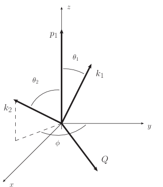
We now turn to the case, where the singularities are due to the three momenta , and . This situation is depicted in Fig. 1. We will use the recursive -dimensional definition of the momentum vectors
| (30) |
Using rotational invariance, we define our momenta as follows
| (31) |
Notice that the sign of is of no relevance for our considerations. We can, for example, assume that and only restore the sign using a reflection transformation at the end. On the other hand, in complete generality. We will further introduce the notation
| (32) |
Note that the variable defined before is now
| (33) | |||||
The fact that the relative angle vanishes only, when and is made explicit in the last row. The three-particle phase space can now be written as follows
| (34) | |||||
where the energy integration range has been described previously, and .
As far as the amplitude is concerned, the singular propagator denominators are
| (35) |
where the signs have been chosen such that the expressions are all positive definite. We have omitted the propagators of the massive particles, since they have identical structure, but the analogues of the variables can never vanish. The first two structures are already fully factorized. Problems arise only in the third and fourth cases.
Let us focus on . We already noted before that the presence of a singularity requires that there be (which is equivalent to ) and . This is an example of a line singularity, since in the three-dimensional space spanned by and , the singularity corresponds to a straight line on the plane. On the other hand, a suitable parameterization would only exploit two variables, in which case the singular limits would be , and , independently of the third parameter needed to cover the whole phase space. In order to obtain such a parameterization, we will perform a variable change. While the choice is not unique, we will use a non-linear variable transformation inspired by that used in [10] in a similar setting
| (36) |
With this variable, the phase space becomes
| (37) | |||||
whereas takes the form
| (38) |
It can be demonstrated that besides the integrable singularities in present explicitly in Eq. (37) (which can be remapped to improve convergence), no other singularities are introduced into the construction. In other words, is not substantial for our discussion.
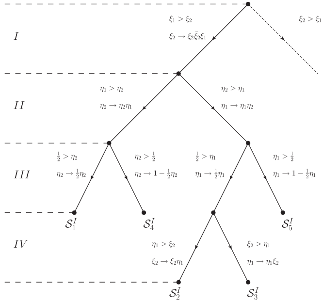
At this point, we are ready to introduce a further decomposition of the phase space that will factorize the invariants given in Eq. (35) and the factor from the phase space measure of Eq. (37) into a product of the integration variables and a function, which does not vanish in any of the singular limits. The decomposition is presented in form of a tree in Fig. 2. For a given ordering of the energies of the massless partons, it contains only five sectors, . In the case of gluons (most intensive from the computational point of view), there is no need to consider the other ordering obtained by symmetry, since the matrix element itself is symmetric. The levels in the decomposition tree have a clear physical interpretation:
-
I)
factorization of the soft singularities;
-
II, III)
factorization of the collinear singularities;
-
IV)
factorization of the soft-collinear singularities.
Each sector specifies an ordering of the relevant variables, thus uniquely defining the limits. Collinear singularities require two levels of decompositions, since besides defining which of the two partons is allowed to become parallel to first, we need to single out the possibility that the partons become collinear to each other first and only then to . This is achieved at level III. An explicit check proves that in all sectors, the necessary factorization is reached. At the same time, the inverse propagators of the massive states responsible for soft singularities are treated at level I.
Let us denote the integration measure obtained from Eq. (37) for a given sector, , by . We consider the contribution of the phase space integral on to an observable, , defined by a measurement function, customarily called jet function, , acting on the phase space. We have
| (39) |
where is a product of the flux, symmetry factors for the final state, and spin and color average factors for the initial state. is the tree-level amplitude with particles. Summation over final state polarizations has been omitted in the notation (it is unnecessary, since the formalism is correct for polarized amplitudes as well). Moreover, as explained in the Introduction, we have ignored the convolution with the PDFs. By construction, we can write the following decomposition
| (40) |
where both and are integers, being defined by alone. To make the decomposition unique, we require first that be regular in the limit of any of the variables vanishing. Furthermore, if a given is divided by one of the four variables, i.e. for some , it is not allowed to vanish, when this variable tends to zero. We would now like to obtain a Laurent expansion in for . The degree of the singularities given by the is crucial to determine the simplest possible construction. Usual general arguments on the IR structure of QCD amplitudes should convince us that , i.e. there are only logarithmic singularities. Thanks to sector decomposition, this statement can be verified explicitly for any amplitude, as we will shortly see. Let us introduce
| (41) |
With this definition, the observable becomes
| (42) |
and the Laurent expansion is obtained by means of the replacement
| (43) |
where , and the “+”-distribution is
| (44) |
The term in Eq. (44) is to be viewed as the subtraction term regularizing the amplitude squared, whereas the term proportional to in Eq. (43) is the integrated subtraction term. The integrated subtraction terms are integrated over the remaining kinematical variables alongside the subtracted amplitude, and no attempt is made at analytic results. After evaluating the integral over the -function, we can even restore the integration sign, since . Notice finally, that the integrated subtraction terms need their own subtraction, which is generated by the same expression. The result is obtained by systematically expanding the expression Eq. (42) (after the substitutions), now a product of polynomials in (we keep only four terms in Eq. (43)), in the latter variable down to the finite part. This is correct, since the generated integrals are convergent by construction. To some extent, viewing this approach as subtraction terms and integrated subtraction terms is inappropriate, but we wish to keep the analogy to the traditional approach.
Up to now, we have worked with an abstract amplitude, which would, however, have to be specified once a definite process would be analyzed. At this point we will make a crucial step in the construction, namely the transition to process independent subtraction. Thanks to the decomposition in terms of physical singularities, each subtraction term generated above and corresponding to one or more of the variables vanishing can be obtained in full generality by means of the known limiting behavior of QCD amplitudes as summarized in [17]. Indeed, will not vanish in the limit, if and only if there is a singularity of the amplitude. The value at this point is obtained at the singularity and the factorization into the tree-level amplitude squared with partons removed times an eikonal factor or splitting function (divided by the singular invariant) applies. Thus the subtraction terms will be given by process specific amplitudes squared (possibly color and/or spin correlated) taken in their reduced kinematics, multiplied by the decomposed product of the measure and eikonal factor or splitting function (divided by the singular invariant). Notice that the reduced kinematics is obtained automatically due to our construction of the phase space (the concept of momentum mapping used in most subtraction schemes is absent here). Moreover, we do not need anymore to think of amplitudes, but only of the eikonal factors and splitting functions. Using their form from [17], it is possible to demonstrate explicitly that is indeed always finite, when one or more variables tend to zero. This proves that divergences are only logarithmic. In summary, the subtraction terms can be determined once and for all. Due to the multitude of cases, the full set is substantially larger than in the next-to-leading order case, but can be derived readily with the information provided above and in [17] by means of simple substitutions (no integration is involved, just simple algebra). To be specific, one should proceed in two steps:
-
1)
Substitute Eqs. (43) and (44) into Eq. (42), while expanding the “+”-distributions. The result contains 16 different objects with vanishing arguments for in all possible combinations. The term with all variables different from zero is the full amplitude squared multiplied by the integration measure.
-
2)
For a given combination of zero arguments of , identify the physical limit and take the appropriate factorization formula from [17]. Subsequently, calculate the limit using the explicit form of the eikonal factor or splitting function. The reduced tree-level amplitude from the factorization formula remains unspecified.
Finally, let us stress that the subtraction terms are local by construction, a crucial feature to assure efficiency. The transverse momentum vectors inducing spin correlations and defining the collinear limits can be derived from the momentum parameterization of Eq. (2.3), and read in the single-collinear limits
| (45) |
where parameterize the transverse direction of with respect to , whereas parameterizes the transverse direction of with respect to at (original variables before sector decomposition), with , and we have assumed . In the triple-collinear limit defined by , const., the normalization of the transverse vectors is not arbitrary. Writing
| (46) | |||||
we can keep as above, if and
| (47) |
where .
2.4 Double-collinear sector
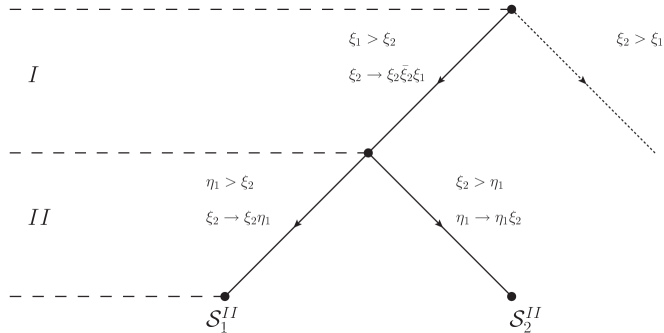
The double-collinear sector can be treated with exactly the same techniques as the triple-collinear sector. For example, the case where the phase space is restricted by , can be obtained with the previous formulae after the replacement . Of course, there are no singularities depending on the value of , which means that one could avoid the non-linear variable change. Moreover, the levels II and III from the decomposition tree of Fig. 2 can be safely removed. In the end there are only two sectors, as given in Fig. 3.
3 Extension to arbitrary final states
It may seem at first that the case of arbitrary final states will be substantially more involved than the one discussed above. However, the only purpose of the restriction to massive states at leading order, was that the system would not cause any collinear or soft singularities. This may be enforced in the most general case by a decomposition of the phase space similar to the one described in Section 2.2. The only difference is that we need more than a constraint on the relative angles.
The double-real radiation at next-to-next-to-leading order is a correction to a leading order process with two massless partons less. The remaining partons need to be well separated and have energies bounded from below. For a jet observable, for example, there may be different ways to enforce this construction. We will assume, however, that we are given a definite set of initial and final states (for a jet observable, there would be a sum over all sub-processes). That is, we need to identify a posteriori the leading order processes possible for the given final state. This is achieved with the help of a jet algorithm together with the requirement that the final state described by jets contain at most two states less than the initial parton configuration.
In order to be able to use the parameterizations and decompositions of the phase space introduced previously, we need to extend the division of the phase space described in Section 2.2. Let denote the set of initial state massless partons, and the set of final state massless partons. The total number of final states is again assumed to be at least four. We define two types of selector functions acting on the phase space: and , both non-negative, with and , and and , , . They are required to satisfy the following conditions with and
| (48) | |||||
and
| (49) |
The selector functions thus define a partition of the phase space. Moreover, inclusion of in the phase space integral allows to obtain a Laurent expansion using the triple-collinear sector decomposition described in Section 2.3, assuming that and take on the role of and , whereas that of . Similarly, allows to obtain a result using the double-collinear sector decomposition from Section 2.4, with corresponding to .
While there is ample freedom in defining the above selector functions, it is possible to extend the NLO construction from [18] to satisfy the above requirements. Let us define
| (50) | |||||
with and the angle between and . Moreover, let
| (51) | |||||
with and , and if . It can readily be verified that the functions
| (52) | |||||
with
| (53) |
We are now able to give the worst case scenario for the number of sectors to consider. At the first stage there are ( and )
| (54) |
triple-collinear sectors and
| (55) |
double-collinear sectors. Counting both stages, the final number is
| (56) |
4 Concluding remarks
The subtraction scheme developed in the previous sections guarantees the possibility to automatically obtain double-real radiation contributions to any observable at NNLO. It is general, just as much as the NLO subtraction schemes, in the sense that the relevant construction is independent of the process.
Notice that we did not consider it important to show that with this construction observables would be finite after combination with the remaining contributions (double-virtual and real-virtual). On the one hand, the correctness of the Laurent expansion obtained with the present method is proven by the correctness of the intermediate steps. The cancellation of the divergences is then guaranteed by the Kinoshita-Lee-Nauenberg and by the factorization theorem. On the other hand, aiming at a proof of cancellation leads to a substantial complication of the scheme. For us, the simplicity of the numerical implementation was of paramount importance. A similar philosophy was already present in the sector decomposition method for phase spaces as devised in [7, 8]. As far as the cancellation of the divergences in dimensional regularization is concerned, a comment is, however, in order. In principle, consistency is guaranteed by the use of the conventional dimensional regularization scheme. This is also implied by our use of formulae from [17]. While our first applications will follow this approach, it is certainly advantageous to use mixed schemes, which would allow to compute all tree level matrix elements in four dimensions, just as it is often done at NLO. Suitable transition formulae, similar to those of [19], will need to be derived in the future.
Finally, let us stress that our scheme is constructed in such a way that the momenta of all partons are available together with the integration weight, which allows to obtain arbitrary distributions on the fly. One may wonder, if the number of sectors will not be a limiting factor to the practical feasibility of the calculation. This should not be the case, since one should consider the sectors as the analogues of the usual phase space channels. In a Monte Carlo implementation one would first choose a sector at random and then the configuration within the sector. The only true measure of complexity is the structure of the subtraction terms. Since they have been derived here using the physical limits it is expected that their number is minimal, and thus the subtraction scheme optimal. Of course, extensions are possible, the most trivial being to add a cut-off on the subtraction phase space. Only practice can show, how important such features will turn out to be.
Acknowledgments
I would like to thank Ch. Anastasiou and G. Heinrich for inspiring discussions, and Z. Trócsányi for interesting correspondence on the content of this letter. Finally, I am grateful to E.W.N. Glover for suggesting the name of the subtraction scheme.
This work was supported by the Heisenberg and by the Gottfried Wilhelm Leibniz programmes of the Deutsche Forschungsgemeinschaft.
References
References
- [1] S. Catani and M. H. Seymour, Nucl. Phys. B 485 (1997) 291 [Erratum-ibid. B 510 (1998) 503];
- [2] S. Catani, S. Dittmaier, M. H. Seymour and Z. Trocsanyi, Nucl. Phys. B 627 (2002) 189;
- [3] M. Czakon, C. G. Papadopoulos and M. Worek, JHEP 0908 (2009) 085;
- [4] S. Frixione, Z. Kunszt and A. Signer, Nucl. Phys. B 467 (1996) 399;
- [5] Z. Nagy and Z. Trocsanyi, Nucl. Phys. B 486 (1997) 189;
- [6] T. Binoth and G. Heinrich, Nucl. Phys. B 585 (2000) 741;
- [7] C. Anastasiou, K. Melnikov and F. Petriello, Phys. Rev. D 69 (2004) 076010;
- [8] T. Binoth and G. Heinrich, Nucl. Phys. B 693 (2004) 134;
- [9] A. Gehrmann-De Ridder, T. Gehrmann and E. W. N. Glover, JHEP 0509 (2005) 056;
- [10] C. Anastasiou, K. Melnikov and F. Petriello, Nucl. Phys. B 724 (2005) 197;
- [11] S. Catani and M. Grazzini, Phys. Rev. Lett. 98 (2007) 222002;
- [12] S. Weinzierl, JHEP 0303 (2003) 062;
- [13] G. Somogyi, Z. Trocsanyi and V. Del Duca, JHEP 0506 (2005) 024;
- [14] F. A. Berends and W. T. Giele, Nucl. Phys. B 313 (1989) 595;
- [15] J. M. Campbell and E. W. N. Glover, Nucl. Phys. B 527 (1998) 264;
- [16] S. Catani and M. Grazzini, Phys. Lett. B 446 (1999) 143;
- [17] S. Catani and M. Grazzini, Nucl. Phys. B 570 (2000) 287;
- [18] S. Frixione, P. Nason and C. Oleari, JHEP 0711 (2007) 070 [arXiv:0709.2092 [hep-ph]].
- [19] S. Catani, M. H. Seymour and Z. Trocsanyi, Phys. Rev. D 55 (1997) 6819.