Abstract

It is shown that the Hubble constant can be derived from the standard luminosity function of galaxies as well as from a new luminosity function as deduced from the mass-luminosity relationship for galaxies. An analytical expression for the Hubble constant can be found from the maximum number of galaxies (in a given solid angle and flux) as a function of the redshift. A second analytical definition of the Hubble constant can be found from the redshift averaged over a given solid angle and flux. The analysis of two luminosity functions for galaxies brings to four the new definitions of the Hubble constant. The equation that regulates the Malmquist bias for galaxies is derived and as a consequence it is possible to extract a complete sample. The application of these new formulae to the data of the two-degree Field Galaxy Redshift Survey provides a Hubble constant of $(65.26\pm 8.22)\mathrm{\ km\ s}^{-1}\mathrm{\ Mpc}^{-1}$ for a redshift lower than 0.042. All the results are deduced in a Euclidean universe because the concept of space-time curvature is not necessary as well as in a static universe because two mechanisms for the redshift of galaxies alternative to the Doppler effect are invoked.

Résumé

Il est montré que la constante de Hubble peut être dêrivé de la fonction de luminositê standard pour les galaxies, ainsi que d’une fonction de luminosité nouvelle dêduite de la relation masse-luminosité pour les galaxies. Une expression analytique de la constante de Hubble peut être trouvêe par rapport au maximum dans le nombre de galaxies (dans un angle solide donné et flux) en fonction du dêcalage vers le rouge . Une deuxiéme dêfinition analytique peut être trouvé par la moyenne de dêcalage vers le rouge d’un angle solide et le flux. Ces deux dêfinitions sont doublêes par l’utilisation d’une fonction de luminositéde nouvelles galaxies. L’êquation qui rêgit le biais Malmquist pour les galaxies est dêrivé et avec comme consêquence est possible d’extraire un êchantillon complet. L’application de ces nouvelles formules pour les donnêes des deux degrês Field Galaxy Redshift Survey fournit une constante de Hubble $(65.26\pm 8.22)\mathrm{\ km\ s}^{-1}\mathrm{\ Mpc}^{-1}$ pour dêcalage vers le rouge infêrieur à 0.042.

KEY WORDS: Distances, redshifts, radial velocities; Observational cosmology

1 Introduction

The Hubble constant, in the following $H_{0}$, is defined as

$$H_{0}=\frac{v}{D}[\mathrm{\ km\ s}^{-1}\mathrm{\ Mpc}^{-1}]\quad,$$ (1)

where $v=cz$ is the recession velocity, $D$ is the distance in $Mpc$, $c$ is the velocity of light and $z$ is the redshift defined as

$$z=\frac{\lambda_{obs}-\lambda_{em}}{\lambda_{em}}\quad,$$ (2)

with $\lambda_{obs}$ and $\lambda_{em}$ denoting respectively the wavelengths of the observed and emitted lines as determined from the lab source. The first numerical values of the Hubble constant were : $H_{0}=625$ $\mathrm{\ km\ s}^{-1}\mathrm{\ Mpc}^{-1}$ as deduced by Lemaitre [1], $H_{0}=460$ $\mathrm{\ km\ s}^{-1}\mathrm{\ Mpc}^{-1}$ as deduced by Robertson [2], $H_{0}=500$ $\mathrm{\ km\ s}^{-1}\mathrm{\ Mpc}^{-1}$ as deduced by Hubble [3] and $H_{0}=290$ $\mathrm{\ km\ s}^{-1}\mathrm{\ Mpc}^{-1}$ as deduced by Oort [4]. Figure 1 reports the decrease of the numerical value of the Hubble constant from 1927 to 1980.

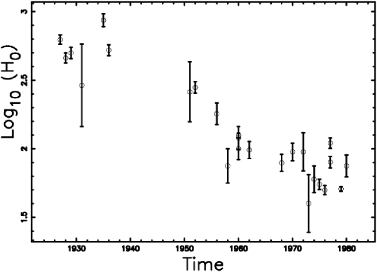
Figure 1: Logarithmic values of the Hubble constant $H_{0}$ from 1927 to 1980. The error bar is evaluated according to the file http://www.cfa.harvard.edu/ huchra/hubble.plot.dat .

At the time of writing, two excellent reviews have been written, see Tammann [5] $(H_{0}=(63.2\pm 1.3~{}(random)~{}\pm 5.3~{}(systematic))$ $\mathrm{\ km\ s}^{-1}\mathrm{\ Mpc}^{-1})$ and Jackson [6] ($H_{0}\sim 70\mbox{\,--\,}73$ $\mathrm{\ km\ s}^{-1}\mathrm{\ Mpc}^{-1}$). We now report the methods that use the global properties of galaxies as indicators of distance:

1. Luminosity classes of spiral galaxies; $H_{0}=(55\pm 3)$ $\mathrm{\ km\ s}^{-1}\mathrm{\ Mpc}^{-1}$ , see Sandage [7]

2. 21 cm line widths; $H_{0}=(59.1\pm 2.5)$ $\mathrm{\ km\ s}^{-1}\mathrm{\ Mpc}^{-1}$ , see Federspiel [8]

3. Brightest cluster galaxies; $H_{0}=(54.2\pm 5.4)$ $\mathrm{\ km\ s}^{-1}\mathrm{\ Mpc}^{-1}$ , see Sandage and Hardy [9]

4. The D_n-$\sigma$ or fundamental plane method; $H_{0}=(57\pm 4)$ $\mathrm{\ km\ s}^{-1}\mathrm{\ Mpc}^{-1}$ , see Federspiel [8]

5. Surface brightness fluctuations; $H_{0}=71.8$ $\mathrm{\ km\ s}^{-1}\mathrm{\ Mpc}^{-1}$ , see Tammann [5]

6. Gravitational lens; $H_{0}=(72\pm 12)$ $\mathrm{\ km\ s}^{-1}\mathrm{\ Mpc}^{-1}$ , see Saha et al. [10]

7. The Sunyaev–Zel’dovich effect; $H_{0}=(67\pm 18)$ $\mathrm{\ km\ s}^{-1}\mathrm{\ Mpc}^{-1}$ , see Udomprasert et al. [11]

8. Ks-band Tully-Fisher Relation; $H_{0}=(84\pm 6)$ $\mathrm{\ km\ s}^{-1}\mathrm{\ Mpc}^{-1}$ , see Russell [12], where the Hubble constant was named Hubble parameter.

At the time of writing, the first important evaluation of the Hubble constant is through Cepheids (key programs with HST) and type Ia Supernovae, see Sandage et al. [13],

$$H_{0}=(62.3\pm 5)\mathrm{\ km\ s}^{-1}\mathrm{\ Mpc}^{-1}\quad.$$ (3)

A second important evaluation comes from the three years of observations with the Wilkinson Microwave Anisotropy Probe, see Table 2 in Spergel et al. [14];

$$H_{0}=(73.2\pm 3.2)\mathrm{\ km\ s}^{-1}\mathrm{\ Mpc}^{-1}\quad.$$ (4)

In the following, we will process galaxies having redshifts as given by the catalog of galaxies. The forthcoming analysis is based on two key assumptions: (i) the flux of radiation from galaxies in a given wavelength decreases with the square of the distance; (ii) the redshift is assumed to have a linear relationship with distance in $Mpc$. These two hypotheses allow some new physical mechanisms to be accepted which produce a linear relationship between redshift and distance, for redshifts lower than 1. In this framework, we can speak of a Euclidean universe because the distances are deduced from the Pythagorean theorem and a static universe because it is not expanding. The already listed approaches leave a series of questions unanswered or partially answered:

• Can the Hubble constant be deduced from the Schechter luminosity function of galaxies?

• Can the Hubble constant be deduced from a new luminosity of galaxies alternative to the Schechter function?

• Can the equation that regulates the Malmquist bias be derived in order to deal with a complete sample in apparent magnitude?

• Can the reference magnitude of the sun be deduced from the luminosity function of galaxies?

In order to answer these questions, Section 2 contains three introductory paragraphs on sample moments, the weighted mean and the determination of the so-called ”exact value” of the Hubble constant. Section 3 reviews the basic system of magnitudes, a review of two alternative mechanisms for the redshift of galaxies, two analytical definitions of the Hubble constant in terms of the Schechter luminosity function of galaxies and two other definitions that can be found by adopting a new luminosity function for galaxies. Section 4 contains a numerical evaluation of the four new formulae for the Hubble constant as deduced from the data of the two-degree Field Galaxy Redshift Survey. Section 5 contains a numerical evaluation of the reference magnitude of the sun for a given catalog.

2 Preliminaries

This Section reviews the evaluation of the first moment about zero and of the second moment about the mean of a sample of data, the evaluation of the mean and variance when each piece of data of a sample has differing errors, the evaluation of the uncertainty and the evaluation of $H_{0}$ from a list of published data.

2.1 Sample moments

Consider a random sample ${\mathcal{X}}=x_{1},x_{2},\dots,x_{n}$ and let $x_{(1)}\geq x_{(2)}\geq\dots\geq x_{(n)}$ denote their order statistics so that $x_{(1)}=\max(x_{1},x_{2},\dots,x_{n})$, $x_{(n)}=\min(x_{1},x_{2},\dots,x_{n})$. The sample mean, $\bar{x}$ , is

$$\bar{x}=\frac{1}{n}\sum{x_{i}}\quad,$$ (5)

and the standard deviation of the sample, $\sigma$ , is according to Press et al. [15]

$$\sigma=\sqrt{\frac{1}{n-1}\sum(x_{i}-\bar{x})^{2}}\quad.$$ (6)

2.2 The weighted mean

The probability, $N(x;\mu,\sigma)$, of a Gaussian (normal) distribution is

$$N(x;\mu,\sigma)=\frac{1}{\sigma(2\pi)^{1/2}}\exp{-{\frac{(x-\mu)^{2}}{2\sigma^{2}}}}\quad,$$ (7)

where $\mu$ is the mean and $\sigma^{2}$ the variance. Consider a random sample ${\mathcal{X}}=x_{1},x_{2},\dots,x_{n}$ where each value is from a Gaussian distribution having the same mean but a different standard deviation $\sigma_{i}$. By the maximum likelihood estimate, in the following MLE [16, 17] an estimate of the weighted mean, $\mu$ , is

$$\mu=\frac{\sum\frac{xi}{\sigma_{i}^{2}}}{\sum\frac{1}{\sigma_{i}^{2}}}\quad,$$ (8)

and an estimate of the error of the weighted mean, $\sigma(\mu)$ ,

$$\sigma(\mu)=\sqrt{\frac{1}{\sum\frac{1}{\sigma_{i}^{2}}}}\quad,$$ (9)

see [18] for a detailed demonstration.

2.3 Error evaluation

When a numerical value of a constant is derived from a theoretical formula, the uncertainty is found from the error propagation equation (often called law of errors of Gauss) when the covariant terms are neglected (see equation (3.14) in [17]). In the presence of more than one evaluation of a constant with different uncertainties, the weighted mean and the error of the weighted mean are found by formulae (8) and (9). In the following, in each diagram we will specify the technique by which the error bars on the derived quantities are derived.

2.4 A first statistical application

The determination of the numerical value of the Hubble constant is an active field of research and the file http://www.cfa.harvard.edu/ huchra/hubble.plot.dat contains a list of 355 published values during the period 1996–2008. Figure 2 reports the frequencies of such values with the superposition of a Gaussian distribution.

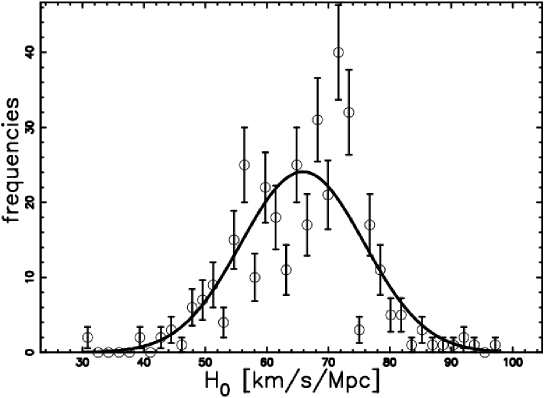
Figure 2: Histogram of frequencies of 355 published values of $H_{0}$ during the period 1996–2008 with error bars computed as the square root of the frequencies. The continuous line fit represents a Gaussian distribution with mean from equation (8) and standard deviation from equation (9) .

Table 1 reports the statistics of this sample as well the minimum, $H_{0,min}$ and maximum $H_{0,max}$ .

Table 1: The Hubble constant from a list of published values during the period 1996–2008.

entity	definition	value
n	No of samples	355
$\bar{x}$	average	65.85 $\mathrm{\ km\ s}^{-1}\mathrm{\ Mpc}^{-1}$
$\sigma$	standard deviation	10 $\mathrm{\ km\ s}^{-1}\mathrm{\ Mpc}^{-1}$
$H_{0},max$	maximum	98 $\mathrm{\ km\ s}^{-1}\mathrm{\ Mpc}^{-1}$
$H_{0},min$	minimum	30 $\mathrm{\ km\ s}^{-1}\mathrm{\ Mpc}^{-1}$
$\mu$	weighted mean	66.04 $\mathrm{\ km\ s}^{-1}\mathrm{\ Mpc}^{-1}$
$\sigma(\mu)$	error of the weighted mean	0.25 $\mathrm{\ km\ s}^{-1}\mathrm{\ Mpc}^{-1}$

3 Useful formulae

This Section reviews three different mechanisms for the redshifts of galaxies: the system of magnitudes, the standard luminosity function in the following LF of galaxies and a new LF of galaxies as given by the mass-luminosity relationship.

3.1 The nature of the redshift

In the following, we will present two theories for the redshift of galaxies alternative to the Doppler effect which are based on basic axioms of physics. In these two alternative mechanisms, the distance, $r$, in a Cartesian coordinate system, $x,y,z$, is given by the usual Pythagorean theorem $r=\sqrt{x^{2}+y^{2}+z^{2}}$. These two alternative theories do not require any expansion of the universe even though local velocities of the order of $\approx~{}100\frac{km}{s}$ are not excluded. These random velocities of galaxies can explain the bending of radiogalaxies, see Zaninetti [19].

Starting from Hubble [3], the suggested correlation between the expansion velocity and distance in the framework of the Doppler effect is

$$V=H_{0}D=c\,z\quad,$$ (10)

where $H_{0}$ is the Hubble constant $H_{0}=100h$ $\mathrm{\ km\ s}^{-1}\mathrm{\ Mpc}^{-1}$ , with $h=1$ when $h$ is not specified, $D$ is the distance in $Mpc$, $c$ is the velocity of light and $z$ the redshift. The quantity $cz$, a velocity, or $z$, a number, characterizes the catalog of galaxies. The Doppler effect produces a linear relationship between distance and redshift. The analysis of mechanisms which predict a direct relationship between distance and redshift started with Marmet [20] and a current list of the various mechanisms can be found in Marmet [21]. Here, we select two mechanisms amongst others. The presence of a hot plasma with low density, such as in the intergalactic medium, produces a relationship of the type

$$D=\frac{{3.0064\cdot 10^{24}}}{{\left({N_{e}}\right)_{av}}}\ln\left({1+z}\right)~{}~{}{\rm{cm}}{\rm{}}\quad,$$ (11)

where the averaged density of electrons, $\left({N_{e}}\right)_{av}$ , is

$$\left({N_{e}}\right)_{av}=\frac{{H_{0}}}{{3.076\cdot 10^{5}}}\approx 2.42\cdot 10^{-4}\left(\frac{{H_{0}}}{{74.5}}\right)\,~{}{\rm{cm}}^{-3}{\rm{,}}$$ (12)

see equations (48) and (49) in Brynjolfsson [22] or equation (27) in Brynjolfsson [23]. A second explanation for the redshift is the Dispersive Extinction Theory (DET) in which the redshift is caused by the dispersive extinction of star light by the intergalactic medium. In this theory

$$z=(\frac{\pi bc}{4})\frac{\delta\lambda^{2}}{\lambda^{3}}D\quad,$$ (13)

where $\delta\lambda$ is the natural linewidth and $b$ is a parameter which characterizes the linearity of the extinction, see formula (17) in Wang [24].

3.2 System of magnitudes

The absolute magnitude of a galaxy, $M$, is connected to the apparent magnitude $m$ through the relationship

$$M=m-5Log(\frac{cz}{H_{0}})-25\quad.$$ (14)

In a Euclidean, non-relativistic and homogeneous universe, the flux of radiation, $f$, expressed in $\frac{L_{\hbox{$\odot$}}}{Mpc^{2}}$ units, where $L_{\hbox{$\odot$}}$ represents the luminosity of the sun, is

$$f=\frac{L}{4\pi D_{L}^{2}}\quad,$$ (15)

where $D_{L}$ represents the distance of the galaxy expressed in $Mpc$ and

$$D_{L}=\frac{cz}{H_{0}}\quad.$$ (16)

The relationship connecting the absolute magnitude, $M$, of a galaxy to its luminosity is

$$\frac{L}{L_{\hbox{$\odot$}}}=10^{0.4(M_{\hbox{$\odot$}}-M)}\quad,$$ (17)

where $M_{\hbox{$\odot$}}$ is the reference magnitude of the sun in the bandpass under consideration.

The flux expressed in $\frac{L_{\hbox{$\odot$}}}{Mpc^{2}}$ units as a function of the apparent magnitude is

$$f=7.957\times 10^{8}\,{e^{0.921\,{\it M_{\hbox{$\odot$}}}-0.921\,{\it m}}}\quad\frac{L_{\hbox{$\odot$}}}{Mpc^{2}}\quad,$$ (18)

and the inverse relationship is

$$m=M_{\hbox{$\odot$}}-1.0857\,\ln\left(0.1256\times 10^{-8}f\right)\quad.$$ (19)

3.3 The Schechter function

The Schechter function, introduced by Schechter [25], provides a useful fit for the luminosity of galaxies

$$\Phi(L)dL=(\frac{\Phi^{*}}{L^{*}})(\frac{L}{L^{*}})^{\alpha}\exp\bigl{(}{-\frac{L}{L^{*}}}\bigr{)}dL\quad.$$ (20)

Here, $\alpha$ sets the slope for low values of $L$, $L^{*}$ is the characteristic luminosity and $\Phi^{*}$ is the normalization. The equivalent distribution in absolute magnitude is

$$\Phi(M)dM= (0.4ln10)\Phi^{*}10^{0.4(\alpha+1)(M^{*}-M)}$$ (21)

$$\times\exp\bigl{(}{-10^{0.4(M^{*}-M)}}\bigr{)}dM\quad,$$

where $M^{*}$ is the characteristic magnitude as derived from the data. The joint distribution in z and f for galaxies, see formula (1.104) in Padmanabhan [26] or formula (1.117) in Padmanabhan [27], is

$$\frac{dN}{d\Omega dzdf}=4\pi\bigl{(}\frac{c}{H_{0}}\bigr{)}^{5}z^{4}\Phi(\frac{z^{2}}{z_{crit}^{2}})\quad,$$ (22)

where $d\Omega$ , $dz$ and $df$ represent the differential of the solid angle, redshift and flux, respectively. This relationship has been derived assuming $z\approx\frac{V}{c}\approx\frac{H_{0}r}{c}$ and using equation (15). The critical value of $z$, $z_{crit}$, is

$$z_{crit}^{2}=\frac{H_{0}^{2}L^{*}}{4\pi fc^{2}}\quad.$$ (23)

The number of galaxies in $z$ and $f$ as given by formula (22) has a maximum at $z=z_{pos-max}$ , where

$$z_{pos-max}=z_{crit}\sqrt{\alpha+2}\quad,$$ (24)

which can be re-expressed as

$$z_{pos-max}=\frac{\sqrt{2+\alpha}\sqrt{{10}^{0.4\,{\it M_{\hbox{$\odot$}}}-0.4\,{\it M^{*}}}}{\it H_{0}}}{2\,\sqrt{\pi}\sqrt{f}{\it c}}\quad.$$ (25)

From the previous formula, it is possible to derive a first Hubble constant adopting for the velocity of light $c=299792.458\mathrm{\frac{km}{s}}$, Mohr and Taylor [28],

$$H_{0}^{I}=\frac{N^{I}}{D^{I}}\mathrm{\ km\ s}^{-1}\mathrm{\ Mpc}^{-1}$$ (26)

$$N^{I}={2.997\times 10^{10}{\it z_{pos-max}}\,\sqrt{{{\rm e}^{0.921{\it M_{\hbox{$\odot$}}}-0.921\,{\it m}}}}}$$

$$D^{I}={\sqrt{2+\alpha}\sqrt{{10}^{0.4\,{\it M_{\hbox{$\odot$}}}-0.4\,{\it M^{*}}}}}\quad.$$

The mean redshift of galaxies with a flux $f$, see formula (1.105) in Padmanabhan [26], or formula (1.119) in Padmanabhan [27] is

$$\langle z\rangle=z_{crit}\frac{\Gamma(3+\alpha)}{\Gamma(5/2+\alpha)}\quad.$$ (27)

A second Hubble constant can be derived from the observed averaged redshift for a given magnitude

$$H_{0}^{II}=\frac{N^{II}}{D^{II}}\mathrm{\ km\ s}^{-1}\mathrm{\ Mpc}^{-1}$$ (28)

$$N^{II}=1.691\,10^{10}{\langle z\rangle}_{obs}\times$$

$$\sqrt{\pi}\sqrt{{{\rm e}^{0.921\,{\it M_{\hbox{$\odot$}}}-0.921\,{\it m}}}}\Gamma\left(5/2+\alpha\right)$$

$$D^{II}={\Gamma\left(3+\alpha\right)\sqrt{{10}^{0.4\,{\it M_{\hbox{$\odot$}}}-0.4\,{\it M^{*}}}}}\quad,$$

where ${\langle z\rangle}_{obs}$ is the averaged redshift as evaluated from the considered catalog.

From formula (27), it is also possible to derive the reference magnitude of the sun $M_{\hbox{$\odot$}}$ for the given catalog

$$M_{\hbox{$\odot$}}=M^{*}+$$

$$1.085\,\ln\left(1.129\times 10^{12}\,{\frac{{{\it{\langle z\rangle}_{obs}}}^{2}f\left(\Gamma\left(2.5+\alpha\right)\right)^{2}}{{{\it H_{0}}}^{2}\left(\Gamma\left(3+\alpha\right)\right)^{2}}}\right)\quad.$$ (29)

In this case, $M_{\hbox{$\odot$}}$ is the unknown and $H_{0}$ is an input parameter.

3.4 The mass-luminosity relationship

A new LF of galaxies as derived in Zaninetti [29] is

$$\Psi(L)dL= (\frac{1}{a\Gamma(c_{f})})(\frac{\Psi^{*}}{L^{*}})\left(\frac{L}{L^{*}}\right)^{\frac{c_{f}-a}{a}}$$ (30)

$$\times\exp\left({-\left(\frac{L}{L^{*}}\right)^{\frac{1}{a}}}\right)dL\quad,$$

where $\Psi^{*}$ is a normalization factor which defines the overall density of galaxies, a number per cubic $Mpc$, $1/a$ is an exponent which connects the mass to the luminosity and $c_{f}$ is connected with the dimensionality of the fragmentation, $c_{f}=2d$, where $d$ represents the dimensionality of the space being considered: 1, 2, 3. The distribution in absolute magnitude is

$$\Psi(M)dM= (0.4ln10\frac{1}{a\Gamma(c_{f})})\Psi^{*}10^{0.4(\frac{c_{f}}{a})(M^{*}-M)}$$ (31)

$$\times\exp\bigl{(}{-10^{0.4(M^{*}-M)(\frac{1}{a})}}\bigr{)}dM\quad.$$

This function contains the parameters $M^{*}$, a, $c_{f}$ and $\Psi^{*}$ which are derived from the operation of fitting the experimental data. The joint distribution in $z$ and $f$, in the presence of the ${\mathcal{M}}-L$ luminosity (equation (30)) is

$$\frac{dN}{d\Omega dzdf}=4\pi\bigl{(}\frac{c}{H_{0}}\bigr{)}^{5}z^{4}\Psi(\frac{z^{2}}{z_{crit}^{2}})\quad.$$ (32)

The number of galaxies, $N_{{\mathcal{M}}-L}(z,f_{min},f_{max})$ comprised between $f_{min}$ and $f_{max}$, can be computed through the following integral

$$N_{{\mathcal{M}}-L}(z)=\int_{f_{min}}^{f_{max}}4\pi\bigl{(}\frac{c}{H_{0}}\bigr{)}^{5}z^{4}\Psi(\frac{z^{2}}{z_{crit}^{2}})df\quad,$$ (33)

and also in this case a numerical integration must be performed.

The number of galaxies as given by formula (32) has a maximum at $z_{pos-max}$ where

$$z_{pos-max}=z_{crit}\left({\it c_{f}}+a\right)^{a/2}\quad,$$ (34)

which can be re-expressed as

$$z_{pos-max}=\frac{\left(a+{\it c_{f}}\right)^{1/2\,a}\sqrt{{10}^{0.4\,{\it M_{\hbox{$\odot$}}}-0.4\,{\it M^{*}}}}{\it H_{0}}}{2\,\sqrt{\pi}\sqrt{f}{\it c}}\quad.$$ (35)

A third Hubble constant as deduced from the maximum in the number of galaxies as a function of z is

$$H_{0}^{III}=\frac{N^{III}}{D^{III}}\mathrm{\ km\ s}^{-1}\mathrm{\ Mpc}^{-1}$$ (36)

$$N^{III}=2.997\times 10^{10}{\it z_{pos-max}}\,\sqrt{{{\rm e}^{0.921\,{\it M_{\hbox{$\odot$}}}-0.921{\it m}}}}$$ (37)

$$D^{III}={\left({\it c_{f}}+a\right)^{0.5\,a}\sqrt{{10.0}^{0.4\,{\it M_{\hbox{$\odot$}}}-0.4\,{\it M^{*}}}}}\quad.$$

The mean redshift connected with the ${\mathcal{M}}-L$ LF is

$$\langle z\rangle=z_{crit}\frac{2\;\;{4}^{-{\frac{2\,a+{\it c_{f}}}{a}}}\Gamma\left(2\,a+{\it c_{f}}\right){2}^{{\frac{2\,{\it c_{f}}+3\,a}{a}}}}{\Gamma\left({\it c_{f}}+3/2\,a\right)}\quad$$ (38)

and the fourth Hubble constant is

$$H_{0}^{IV}=\frac{N^{IV}}{D^{IV}}\mathrm{\ km\ s}^{-1}\mathrm{\ Mpc}^{-1}$$ (39)

$$N^{IV}=8.457\,10^{9}{\it{\langle z\rangle}_{obs}}\times$$

$$\sqrt{\pi}\sqrt{{{\rm e}^{0.921\,{\it M_{\hbox{$\odot$}}}-0.921,{\it m}}}}\Gamma\left({\it c_{f}}+3/2\,a\right)$$

$$D^{IV}={4}^{-{\frac{2\,a+{\it c_{f}}}{a}}}\sqrt{{10}^{0.4\,{\it M_{\hbox{$\odot$}}}-0.4\,{\it M^{*}}}}\times$$

$$\Gamma\left(2\,a+{\it c_{f}}\right){2}^{{\frac{2\,{\it c_{f}}+3\,a}{a}}}\quad.$$

4 Numerical value of the Hubble constant

The formulae previously derived are now tested on the catalog from the two-degree Field Galaxy Redshift Survey, in the following 2dFGRS, available at the web site: http://msowww.anu.edu.au/2dFGRS/. In particular we added together the file parent.ngp.txt which contains 145,652 entries for NGP strip sources and the file parent.sgp.txt which contains 204,490 entries for SGP strip sources. Once the heliocentric redshift was selected, we processed 219,107 galaxies with $0.001\leq z\leq 0.3$ and two strips of the 2dFGRS are shown in Figure 3.

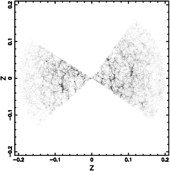
Figure 3: Cone-diagram of all the galaxies in the 2dFGRS. This plot contains 203,249 galaxies.

From the previous Figure is clear the nonhomogeneous structure of the universe and this concept can be clarified by counting the number of galaxies in one of the two slices as a function of the redshift when a sector with a central angle of $1^{\circ}$ is considered, see Figure 4.

Figure 4: Histogram (step-diagram) of the number of galaxies as a function of the redshift in the slice to the right of Figure 3, the number of bins is 50. The circular sector has a central angle of $1^{\circ}$.

Conversely, when the two slices are considered together the behavior of the number of galaxies as a function of the redshift is more continuous, see Figure 5.

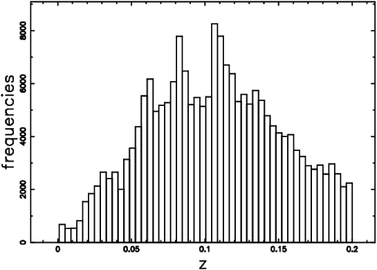
Figure 5: Histogram (step-diagram) of the number of galaxies as a function of the redshift when the two slices of Figure 3 are added together, the number of bins is 50.

In this quasi-homogeneous universe, some statistical properties such as the theoretical position of the maximum in the number of galaxies agree with the observations and Figure 6 reports the observed maximum in the 2dFGRS as well as the theoretical curve as a function of the magnitude.

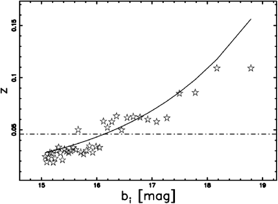
Figure 6: Value of $\widehat{z}_{pos-max}$ at which the number of galaxies in the 2dFGRS is maximum as a function of the apparent magnitude b_J (stars) and theoretical curve of the maximum for the Schechter function as represented by formula (25) (full line). In this plot, $\mathcal{M_{\hbox{$\odot$}}}$ = 5.33 and $H_{0}=65.26\mathrm{\ km\ s}^{-1}\mathrm{\ Mpc}^{-1}$. The horizontal dotted line represents the boundary between complete and incomplete samples.

Before reducing the data, we should discuss the Malmquist bias, see Malmquist [30, 31], which was originally applied to the stars and was then applied to the galaxies by Behr [32]. We therefore introduce the concept of limiting apparent magnitude and the corresponding completeness in absolute magnitude of the considered catalog as a function of the redshift. The observable absolute magnitude as a function of the limiting apparent magnitude, $m_{L}$, is

$$M_{L}=m_{{L}}-5\,{\it\log_{10}}\left({\frac{{\it c}\,z}{H_{{0}}}}\right)-25\quad.$$ (40)

The previous formula predicts, from a theoretical point of view, an upper limit on the absolute maximum magnitude that can be observed in a catalog of galaxies characterized by a given limiting magnitude and Figure 7 reports such a curve and the galaxies of the 2dFGRS.

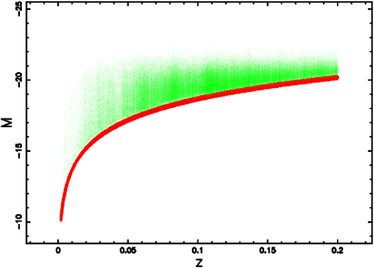
Figure 7: The absolute magnitude $M$ of 202,923 galaxies belonging to the 2dFGRS when $\mathcal{M_{\hbox{$\odot$}}}$ = 5.33 and $H_{0}=66.04\mathrm{\ km\ s}^{-1}\mathrm{\ Mpc}^{-1}$ (green points). The upper theoretical curve as represented by equation (40) is reported as the red thick line when $m_{L}$=19.61.

The interval covered by the LF of galaxies, $\Delta M$, is defined by

$$\Delta M=M_{max}-M_{min}\quad,$$ (41)

where $M_{max}$ and $M_{min}$ are the maximum and minimum absolute magnitude of the LF for the considered catalog. The real observable interval in absolute magnitude, $\Delta M_{L}$, is

$$\Delta M_{L}=M_{L}-M_{min}\quad.$$ (42)

We can therefore introduce the range of observable absolute maximum magnitude expressed in percent, $\epsilon_{s}(z)$, as

$$\epsilon_{s}(z)=\frac{\Delta M_{L}}{\Delta M}\times 100\,\%\quad.$$ (43)

This is a number that represents the completeness of the sample and, given the fact that the limiting magnitude of the 2dFGRS is $m_{L}$=19.61, it is possible to conclude that the 2dFGRS is complete for $z\leq 0.0442$ . This efficiency expressed as a percentage can be considered a version of the Malmquist bias. In our case, we have chosen to process the galaxies of the 2dFGRS with $z\leq 0.0442$ of which there are 22,071: in other words our sample is complete. Another quantity that should be fixed in order to continue is the absolute magnitude of the sun in the b_J filter, $\mathcal{M_{\hbox{$\odot$}}}$ = 5.33, see Colless et al. [33], Tempel et al. [34], Eke et al. [35].

We now outline the algorithm that allows to deduce $z_{pos-max}$ and ${\langle z\rangle}_{obs}$ from a catalog of galaxies.

1. We fix a given flux or magnitude, for example b_J, and a relative narrow window.

2. We organize the selected galaxies according to frequency versus redshift, see a typical histogram in Figure 8.

3. Once the histogram is made, we compute the astronomical $z=z_{pos-max}$, which is inserted in formulae (26) and (36) in order to deduce the Hubble constant.

4. The selected sample of galaxies with a given magnitude allows an easy determination of ${\langle z\rangle}_{obs}$.

5. Particular attention should be paid to the completeness of the sample and Figure 9 reports the maximum value in redshift $z_{max}$ for each run in magnitude/flux.

Table 2 reports the four values of the Hubble constant deduced here and Figure 10 displays the data corresponding to the constant deduced from equation (28).

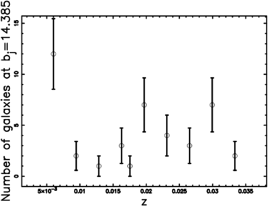
Figure 8: The galaxies of the 2dFGRS, with $\mbox{b${}_{\rm\scriptscriptstyle J}$}\approx 14.385$ or $f$ $\approx 189983\frac{L_{\hbox{$\odot$}}}{Mpc^{2}}$, are isolated in order to represent a chosen value of $m$ or $f$ and then organized according to frequency versus heliocentric redshift. The error bars are computed as the square root of the frequencies. The maximum in the frequency of observed galaxies is at $z=0.006$ when $\mathcal{M_{\hbox{$\odot$}}}$ = 5.33 .

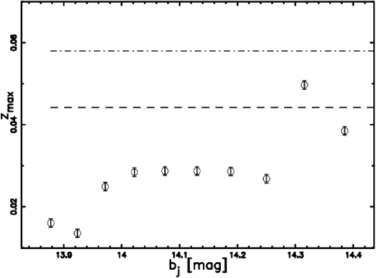
Figure 9: Plot of $z_{max}$ as a function of the chosen magnitude (empty stars). The error bar in $z$ is computed as the width of the bin. The dashed line represents the lower limit of the complete sample, $\epsilon_{s}(z)=100\%$, and the dash-dot-dash line corresponds to $\epsilon_{s}(z)=90\%$.

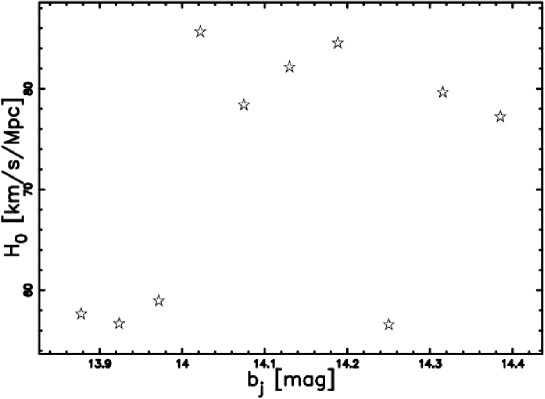
Figure 10: The Hubble constant as deduced by the second method, see equation (28), as a function of the selected magnitude (empty stars).

Table 2: Numerical values of the Hubble constant as deduced from 10 different apparent magnitudes.

	LF	matching $z$	[$\mathrm{\ km\ s}^{-1}\mathrm{\ Mpc}^{-1}]$
1	Schechter	$z_{pos-max}$	( 58.35 $\pm$ 30 )
2	Schechter	${\langle z\rangle}_{obs}$	( 71.73$\pm$ 12)
3	${\mathcal{M}}-L$	$z_{pos-max}$	( 60.72 $\pm$ 32)
4	${\mathcal{M}}-L$	${\langle z\rangle}_{obs}$	( 71.20 $\pm$ 12 )
5	weighted mean		( 65.26 $\pm$ 8.22 )
6	sample mean		(62.88 $\pm$ 6.0 )

From a practical point of view, $\epsilon$, the percentage reliability of our results can also be introduced,

$$\epsilon=(1-\frac{|(Q_{obs}-Q_{num})|}{Q_{obs}})\cdot 100\,\%\,,$$ (44)

where $Q_{obs}$ is the quantity given by the astronomical observations and $Q_{num}$ is the analogous quantity calculated by us. The value of $H_{0}$ as found by us with the weighted mean is, see fifth row in Table 2, $H_{0}=65.26\mathrm{\ km\ s}^{-1}\mathrm{\ Mpc}^{-1}$ and the observed value, see the weighted mean in Table 1, $H_{0}=66.04\mathrm{\ km\ s}^{-1}\mathrm{\ Mpc}^{-1}$ .

5 The absolute magnitude of the sun

The reference absolute magnitude of the sun (the unknown variable) can be derived from formula (29) but in this case the value of $H_{0}$ (known variable) should be specified. Perhaps the best choice is the weighted mean reported in Table (1), $H_{0}=66.04\mathrm{\ km\ s}^{-1}\mathrm{\ Mpc}^{-1}$. Adopting this value of $H_{0}$, the absolute reference magnitude of the sun can be plotted in Figure 11 and the averaged value is

$$\overline{M_{\hbox{$\odot$}}}=(5.50\pm 0.35)mag\quad.$$ (45)

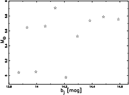
Figure 11: The absolute reference magnitude of the sun, equation (29), as a function of the selected magnitude (empty stars).

The efficiency in deriving the absolute reference magnitude of the sun is

$$\epsilon=96.63~{}\%\quad.$$ (46)

6 Conclusions

A careful study of the standard LF of galaxies allows the determination of the position of the maximum in the theoretical number of galaxies versus redshift and the theoretical averaged redshift. From the two previous analytical results, it is possible to extract two new formulae for the Hubble constant, equations (26) and (28). The same procedure can be applied by analogy to a new LF as given by the mass-luminosity relationship, see equations (36) and (39). The weighted mean of the four values of $H_{0}$ as deduced from Table 2 gives

$$H_{0}=(65.26\pm 8.22)\mathrm{\ km\ s}^{-1}\mathrm{\ Mpc}^{-1}\quad when~{}z\leq 0.042\quad.$$

This value lies between the value deduced from the Cepheids, see Sandage et al. [13] and formula (3) and the value deduced from WMAP,

see Spergel et al. [14] and formula (4).

The developed framework also enables the deduction of the reference magnitude of the sun, see formula (29) and the application to the 2dFGRS gives

$$M_{\hbox{$\odot$}}=(5.5\pm 0.35)\quad.$$ (47)

Assuming that the exact value is $M_{\hbox{$\odot$}}$ = 5.33, the efficiency in deriving the reference magnitude of the sun is $\epsilon=96.63~{}\%$ when $H_{0}=66.04\mathrm{\ km\ s}^{-1}\mathrm{\ Mpc}^{-1}$. We briefly review the basic cosmological assumptions adopted here to derive the Hubble constant:

• The mechanism that produces the redshift, here extracted from the catalog of galaxies, is not specified but we remember that the plasma redshift and DET (Dispersive Estinction Theory) do not produce a geocentric model for the universe as given by the Doppler shift, see Wang [36].

• The number of galaxies as a function of redshift as well as the averaged redshift are evaluated in a Euclidean space or, in other words, the effects of space-curvature are ignored.

• The spatial inhomogeneities present in the catalog of galaxies are partially neutralized by the operation of adding together the data of the south and north galactic pole of the 2dFGRS. The transition from a nonhomogeneous to a quasi-homogeneous universe is clear when Figure 5 and Figure 4 are carefully analyzed.

• The initial assumptions of: (i) natural flux decreasing as given by equation (15) ; (ii) linear relationship between redshift and distance which are present in the joint distribution in z and f for the number of galaxies are justified by the acceptable results obtained for the theoretical maximum in the number of galaxies, see Figure 6. This fact allow us to speak of a Euclidean universe up to $z\leq 0.042$.

• The presence of the Malmquist bias does not allow to extrapolate the concept of a Euclidean, static universe for distances greater than $z\,>\,0.042$ when the 2dFGRS catalog is considered.

References

- Lemaitre [1927] G. Lemaitre, Ann. Soc. Sci. Bruxelles 47A, 49 (1927).
- Robertson [1928] H. Robertson, Phil. Mag. 5, 835 (1928).
- Hubble [1929] E. Hubble, Proc. Natl. Acad. Sci. 15, 168 (1929).
- Oort [1931] J. H. Oort, BAN 6, 155 (1931).
- Tammann [2006] G. A. Tammann, in Reviews in Modern Astronomy, edited by S. Roeser (2006), vol. 19 of Reviews in Modern Astronomy, pp. 1–+.
- Jackson [2007] N. Jackson, Living Reviews in Relativity 10, 4 (2007), 0709.3924.
- Sandage [1999] A. Sandage, ApJ 527, 479 (1999).
- Federspiel [1999] M. Federspiel, Ph.D. thesis, Univ. of Basel (1999).
- Sandage and Hardy [1973] A. Sandage and E. Hardy, ApJ 183, 743 (1973).
- Saha et al. [2006] P. Saha, J. Coles, A. Macció, and L. Williams, Astrophys. J. Lett. 650, L17 (2006).
- Udomprasert et al. [2004] P. Udomprasert, B. Mason, A. Readhead, and T. Pearson, ApJ 615, 63 (2004), arXiv:astro-ph/0408005.
- Russell [2009] D. Russell, J. Astrophys. and Astron. 30, 93 (2009).
- Sandage et al. [2006] A. Sandage, G. A. Tammann, A. Saha, B. Reindl, F. D. Macchetto, and N. Panagia, ApJ 653, 843 (2006), arXiv:astro-ph/0603647.
- Spergel et al. [2007] D. N. Spergel, R. Bean, O. Doré, M. R. Nolta, and C. L. E. A. Bennett, ApJS 170, 377 (2007), arXiv:astro-ph/0603449.
- Press et al. [1992] W. H. Press, S. A. Teukolsky, W. T. Vetterling, and B. P. Flannery, Numerical recipes in FORTRAN. The art of scientific computing (Cambridge University Press, Cambridge, 1992).
- J. V. Wall and C. R. Jenkins [2003] J. V. Wall and C. R. Jenkins, Practical Statistics for Astronomers (Cambridge University Press, Cambridge, 2003).
- P. R. Bevington and D. K. Robinson [2003] P. R. Bevington and D. K. Robinson, Data reduction and error analysis for the physical sciences (McGraw-Hill, New York, 2003).
- W. R. Leo [1994] W. R. Leo, Techniques for Nuclear and Particle Physics Experiments (Springer, Berlin, 1994).
- Zaninetti [2007] L. Zaninetti, Revista Mexicana de Astronomia y Astrofisica 43, 59 (2007).
- Marmet [1988] P. Marmet, Physics Essays 1, 24 (1988).
- Marmet [2009] L. Marmet, in Astronomical Society of the Pacific Conference Series, edited by F. Potter (2009), vol. 413 of Astronomical Society of the Pacific Conference Series, pp. 315–+.
- Brynjolfsson [2004] A. Brynjolfsson, arXiv:astro-ph/0401420 (2004), arXiv:astro-ph/0401420.
- Brynjolfsson [2009] A. Brynjolfsson, in Astronomical Society of the Pacific Conference Series, edited by F. Potter (2009), vol. 413 of Astronomical Society of the Pacific Conference Series, pp. 169–+.
- Wang [2005] L. J. Wang, Physics Essays 18, 177 (2005).
- Schechter [1976] P. Schechter, ApJ 203, 297 (1976).
- Padmanabhan [1996] T. Padmanabhan, Cosmology and Astrophysics through Problems (Cambridge University Press, Cambridge, 1996).
- Padmanabhan [2002] P. Padmanabhan, Theoretical astrophysics. Vol. III: Galaxies and Cosmology (Cambridge University Press, Cambridge, MA, 2002).
- Mohr and Taylor [2005] P. J. Mohr and B. N. Taylor, Rev. Mod. Phys. 77, 1 (2005).
- Zaninetti [2008] L. Zaninetti, AJ 135, 1264 (2008).
- Malmquist [1920] K. Malmquist , Lund Medd. Ser. II 22, 1 (1920).
- Malmquist [1922] K. Malmquist , Lund Medd. Ser. I 100, 1 (1922).
- Behr [1951] A. Behr, Astronomische Nachrichten 279, 97 (1951).
- Colless et al. [2001] M. Colless, G. Dalton, S. Maddox, et al., MNRAS 328, 1039 (2001), astro-ph/0106498.
- Tempel et al. [2009] E. Tempel, J. Einasto, M. Einasto, E. Saar, and E. Tago, A&A 495, 37 (2009), 0805.4264.
- Eke et al. [2004] V. R. Eke, C. S. Frenk, C. M. Baugh, S. Cole, and P. Norberg, MNRAS 355, 769 (2004), arXiv:astro-ph/0402566.
- Wang [2007] L. J. Wang, Physics Essays 20, 329 (2007).