Galaxy Clustering Topology in the Sloan Digital Sky Survey Main Galaxy Sample: a Test for Galaxy Formation Models

Yun-Young Choi¹¹affiliation: Dept. of Astronomy & Space Science, Kyung Hee University, Gyeonggi 446-701, Korea , Changbom Park²²affiliation: Korea Institute for Advanced Study, Dongdaemun-gu, Seoul 130-722, Korea , Juhan Kim¹¹affiliation: Dept. of Astronomy & Space Science, Kyung Hee University, Gyeonggi 446-701, Korea , J. Richard Gott III³³affiliation: Department of Astrophysical Sciences, Peyton Hall, Princeton University, Princeton, NJ 08544-1001, USA , David H. Weinberg⁴⁴affiliation: Department of Astronomy and CCAPP, Ohio State University, Columbus, OH 43210. , Michael S. Vogeley⁵⁵affiliation: Department of Physics, Drexel University, 3141 Chestnut Street, Philadelphia, PA 19104, USA , and Sungsoo S. Kim¹¹affiliation: Dept. of Astronomy & Space Science, Kyung Hee University, Gyeonggi 446-701, Korea ⁶⁶affiliation: School of Space Research, Kyung Hee University, Yongin, Gyeonggi 446-701, Korea
(for the SDSS Collaboration)

Abstract

We measure the topology of the main galaxy distribution using the Seventh Data Release of the Sloan Digital Sky Survey, examining the dependence of galaxy clustering topology on galaxy properties. The observational results are used to test galaxy formation models. A volume-limited sample defined by $M_{r}<-20.19$ enables us to measure the genus curve with amplitude of $G=378$ at $6h^{-1}$ Mpc smoothing scale, with 4.8% uncertainty including all systematics and cosmic variance. The clustering topology over the smoothing length interval from 6 to $10h^{-1}$ Mpc reveals a mild scale-dependence for the shift ( $\Delta\nu$ ) and void abundance ( $A_{V}$ ) parameters of the genus curve. We find substantial bias in the topology of galaxy clustering with respect to the predicted topology of the matter distribution, which varies with luminosity, morphology, color, and the smoothing scale of the density field. The distribution of relatively brighter galaxies shows a greater prevalence of isolated clusters and more percolated voids. Even though early (late)-type galaxies show topology similar to that of red (blue) galaxies, the morphology dependence of topology is not identical to the color dependence. In particular, the void abundance parameter $A_{V}$ depends on morphology more strongly than on color. We test five galaxy assignment schemes applied to cosmological N-body simulations of a $\Lambda$ CDM universe to generate mock galaxies: the Halo-Galaxy one-to-one Correspondence model, the Halo Occupation Distribution model, and three implementations of Semi-Analytic Models (SAMs). None of the models reproduces all aspects of the observed clustering topology; the deviations vary from one model to another but include statistically significant discrepancies in the abundance of isolated voids or isolated clusters and the amplitude and overall shift of the genus curve. SAM predictions of the topology color-dependence are usually correct in sign but incorrect in magnitude. Our topology tests indicate that, in these models, voids should be emptier and more connected, and the threshold for galaxy formation should be at lower densities.

Subject headings:

large-scale structure of universe – cosmology: observations – methods: numerical

1. Introduction

Galaxy clustering has long been used to constrain cosmological models and to understand formation of galaxies. The most extensively studied clustering statistics are the autocorrelation function and the power spectrum. They are Fourier transforms of each other, and measure the clustering strength as a function of scale. The “Standard Cold Dark Matter” model (with the density parameter $\Omega_{m}=1$ , scale-invariant primordial fluctuations, and standard relativistic particle background), popular in the 1980s, was ruled out by showing that it was inconsistent with the observed galaxy correlation function (Maddox et al. 1990) and power spectrum (Vogeley et al. 1992; Park et al. 1992, 1994). These statistics are also used to measure the biasing in the galaxy clustering amplitude with respect to matter, and are key constraints on galaxy formation models connecting dark matter halos and luminous galaxies such as semi-analytic models (SAM; e.g., White & Frenk 1991; Kauffmann et al. 1993; Cole et al. 1994, 2000; Benson et al. 2002; Bower et al. 2006; Cattaneo et al. 2006; Croton et al. 2006; De Lucia & Blaizot 2007; Monaco et al. 2007; Somerville et al. 2008) and halo occupation distribution models (e.g., Seljak 2000; Peacock & Smith 2000; Scoccimarro et al. 2001; Berlind & Weinberg 2002; Kang et al. 2002; Berlind et al. 2003; Zheng, Coil, & Zehavi 2007).

Topology analysis was introduced by Gott et al. (1986, 1987) to test the Gaussianity of the primordial density fluctuations, which is one of the key characteristics of simple inflationary models (Bardeen et al. 1986). At large scales density fluctuations are still in the linear regime and maintain their initial topology, and it is possible to check whether or not the primordial fluctuations were a Gaussian field. At smaller scales, non-linear gravitational evolution and biased galaxy formation make the topology of the observed galaxy distribution deviate from the Gaussian form even if the initial conditions were Gaussian distributed as shown by perturbation theories and large N-body simulations (Park & Gott 1991; Weinberg & Cole 1992; Matsubara 1994; Matsubara & Suto 1996); using fractional volume rather than density threshold as the independent variable in topology analysis mitigates but does not eliminate these non-linear and biasing effects (Weinberg et al. 1987; Melott et al. 1988). Through studies of many observational samples, the topological properties of the large-scale distribution of galaxies have been examined (Gott et al. 1989; Park, Gott & da Costa 1992; Moore et al. 1992; Vogeley et al. 1994; Rhoads, Gott, & Postman 1994; Protogeros & Weinberg 1997; Canavezes et al. 1998; Park, Gott & Choi 2001; Hoyle, Vogeley & Gott 2002; Hikage et al. 2002, 2003; Park et al. 2005; James, Lewis & Colless 2007; Gott, Choi & Park 2009; James et al. 2009). On non-linear or quasi-linear scales, topology analysis is useful in constraining both cosmological parameters and galaxy formation mechanisms (Park, Kim & Gott 2005; Gott et al. 2008). In particular, differences in clustering topology for different types of galaxies reflect their different history of formation and evolution. Therefore, looking at the topology of large-scale structure traced by different types of galaxies can put strong constraints on galaxy formation mechanisms.

In this paper we use the Seventh Data Release (DR7; Abazajian et al. 2009) of the Sloan Digital Sky Survey (York et al. 2000) to measure the topology of the galaxy distribution and its dependence on galaxy luminosity, color, and morphology. DR7 constitutes the final release of the SDSS Legacy Survey, and thus of the main SDSS galaxy redshift survey. We supplement the SDSS data with missing redshifts to increase the completeness of the redshift catalog. We then generate a set of volume-limited samples of the SDSS galaxies divided according to their luminosity, morphology, and color to study the relation between the topology and properties of galaxies tracing the large-scale structure.

2. The KIAS-VAGC catalog

We prepare a catalog containing 593,514 redshifts of the SDSS (York et al. 2002; Stoughton et al. 2002) main galaxies (Strauss et al. 2002) in the magnitude range of $10<r\leq 17.6$ , which is called the Korea Institute for Advanced Study (KIAS) Value-Added Galaxy Catalog (VAGC) (Choi et al. 2010). Its main source is the New York University VAGC Large Scale Structure Sample (brvoid0) from Blanton et al. (2005), which lists redshifts of 583,946 galaxies with $10<r\leq 17.6$ (8,562 with $10<r\leq 14.5$ ). We excluded 929 objects that are in error. They are outer parts of large galaxies that are deblended by the automated photometric pipeline, blank fields, or stars, etc. Out of the remaining 583,017 galaxies, 5.7% of galaxies in the NYU VAGC LSS do not have spectra due to fiber collision and have redshifts borrowed from the nearest neighbor galaxy. We added redshifts of 10,497 galaxies with $10<r\leq 17.6$ (1,455 with $10<r\leq 14.5$ ) to the KIAS VAGC that are missing in the NYU VAGC LSS. An SDSS photometric catalog and various existing redshift catalogs such as the Updated Zwicky Catalog (UZC; Falco et al. 1999), the IRAS Point Source Catalog Redshift Survey (PSCz; Saunders et al. 2000), the Third Reference Catalogue of Bright Galaxies (RC3; de Vaucouleurs et al. 1991), and the Two Degree Field Galaxy Redshift Survey (2dFGRS; Colless et al. 2001) are used in this step. During this supplementation process, we corrected positions of galaxies having wrong central positions, separated merging objects, and removed spurious objects such as parts of big late-type galaxies. The angular survey mask given by NYU-VAGC is maintained and covers 2.562 sr of sky with angular selection function greater than 0. While the SDSS main galaxy sample extends to $r=17.77$ over most of the sky, we retain the shallower limit $r=17.60$ used during the early part of the survey (see Strauss et al. 2002) to maintain a homogeneous depth of the survey volume and thus a less complicated outer boundary. Extending to $r=17.77$ would add roughly $114,303$ galaxies (from NYU VAGC LSS full0 sample).

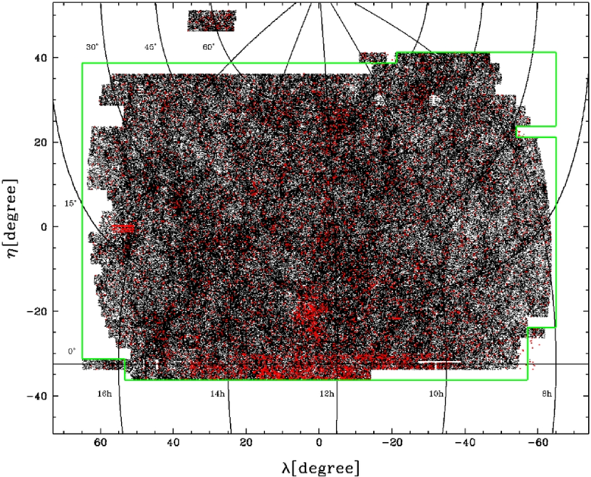
Refer to caption — Figure 1.— SDSS galaxies in the northern galactic hemisphere. Black points are the galaxies in the NYU VAGC LSS catalog and red points are those newly added in the KIAS-VAGC. Green solid lines delineate the boundaries of the analysis regions. $(\eta,\lambda)$ are the SDSS survey coordinates. Lines of constant RA and DEC lines are shown in black as roughly vertical and horizontal curves, respectively.

The resulting KIAS VAGC has an angular selection function significantly better than the original NYU VAGC LSS sample in high surface density regions. Figure 1 shows the distribution of the SDSS galaxies in the northern galactic hemisphere. To minimize boundary effects and to keep the surface-to-volume ratio low in our topology analysis, we do not use the galaxies in three narrow stripes of the southern Galactic cap and in the small region containing the Hubble Deep Field, and we trimmed some regions with narrow angular extent. What remains are the galaxies inside the green solid boundary shown in Figure 1. The remaining survey region with the angular selection function greater than 0 covers 2.33 str. Black points in Figure 1 are the galaxies in NYU VAGC LSS catalog and red points are those newly added. It can be seen that the added galaxies are mostly located in high surface density regions. In particular, a large number of galaxies are added in the Virgo cluster region and near the equator. Correspondingly, we recalculate the angular selection function of the KIAS VAGC within each spherical polygon formed by the adaptive tiling algorithm (Blanton et al. 2003) used for the SDSS spectroscopy. Choi et al. (2010) show the angular selection function before and after supplementation. After the supplementation, the survey area (in the northern hemisphere) having angular selection function greater than 0.97 increases from 39.8% to 54.3% of the area with the selection function greater than 0.

All atlas images of galaxies in our KIAS VAGC are downloaded from Princeton SDSS reduction server¹¹1http://photo.astro.princeton.edu and analyzed to measure the seeing- and inclination-corrected $i$ -band Petrosian radius, $i$ -band inverse concentration index, $c_{\rm in}$ and $\Delta(g-i)$ color gradient (Park & Choi 2005; Choi et al. 2007). These parameters are included in KIAS VAGC together with other fundamental photometric and spectroscopic parameters supplied by the NYU VAGC.

All galaxies in KIAS VAGC are classified into early (elliptical and lenticular) and late (spiral and irregular) morphological types. We use the automated classification scheme developed by Park & Choi (2005) using $u-r$ color, $\Delta(g-i)$ color gradient, and the inverse concentration index $c_{\rm in}$ . Reliability and completeness of this classification reach about 90%. To improve the automated classification results by visual inspection we selected 82,323 galaxies that are located in the “trouble zones” where the reliability of the automated classification is low. These are the galaxies having neighbors at very small separations (for these $c_{\rm in}$ is inaccurate) or those classified as blue early types or red late types. Thirteen astronomers made the visual inspection to check the morphological type of these galaxies. As a result, the morphology of 7% of the inspected galaxies was changed and some spurious objects are removed. We kept the morphology of 5,956 galaxies in the SDSS LSS-DR4plus sample that were already inspected by Choi et al. (2007).

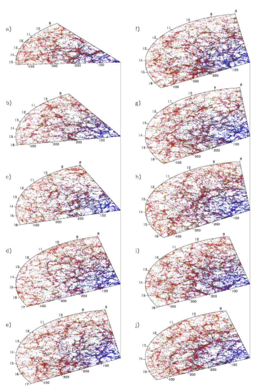
Figure 2 shows the galaxies of the KIAS-VAGC contained in ten consecutive wedge slices in the main survey area. Each slice has the radius of 450 $h^{-1}$ Mpc and is 6 degree thick in declination. The range in right ascension is varied according to the survey boundaries shown in Figure 1. The right ascension and declination ranges and the number of galaxies in each slice are listed in Table 1. Galaxies are distinguished according to their color: blue is given to those with $u-r<2.0$ , green is for $2.0\leq u-r<2.5$ , and red is for $u-r\geq 2.5$ . Since we are showing galaxies in the apparent magnitude-limited sample, galaxies are on average faint and blue at small distances and bright and red at large distances. A part of the Sloan Great Wall (Gott et al. 2005) is seen in the bottom slice (slice j, at $r\approx 250h^{-1}\,$ Mpc), and the CfA Great Wall (Geller & Huchra 1989) appears in slice e at $r\approx 100h^{-1}\,$ Mpc. A part of the Cosmic Runner (Park et al. 2005) shows up in the top slice a. There are also numerous prominent superclusters, notably a group of superclusters in slice f and a few rod-shaped ones in slice i. In addition to these large scale overdense structures, many large voids are prevalent in the survey volume. It should be also noted that none of these features really stands out any more; the Sloan Great Wall is just a high end of the distribution of structures that are quite common. A weak circular symmetry around the observer is seen in slice j, but we do not have such impression in other slices.

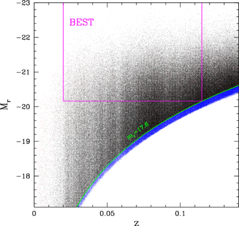
We will use several volume-limited samples defined by $r$ -band absolute magnitude cuts and the redshift limits of $z_{\rm min}=0.02$ and $z_{\rm max}$ , where $z_{\rm max}$ is determined by the survey flux limit $r=17.6$ and the absolute magnitude cut. We frequently refer to the “mean separation” between galaxies in a sample, by which we mean $\bar{d}\equiv n_{g}^{-1/3}$ where $n_{g}$ is the number density of galaxies. Figure 3 shows the galaxies in our catalog in the redshift versus $r$ -band absolute magnitude ( $M_{r}$ ) plane and the boundary lines defining one of our volume-limited samples “BEST”, which contains the maximum number of galaxies (133,947) among volume-limited samples. It is amusing to note that the BEST sample is about 1000 times larger than the galaxy sample (drawn from the CfA1 redshift survey) first used for topological analysis by Gott et al. (1986, 1987).

The WMAP 3 year cosmological parameters of $\Omega_{m}=0.27,\Omega_{\Lambda}=0.73,\Omega_{b}=0.044,h=0.72,n{{}_{s}}=0.958$ (Spergel et al. 2007) are used to relate redshift and comoving distance.

Table 1Survey Regions for the Wedge Diagrams in Figure 2

Panel Name	Right Ascension	Declination	Num. of galaxies
a	$8.5^{\circ}-15.3^{\circ}$	$54^{\circ}-60^{\circ}$	22,237
b	$8.5^{\circ}-16.0^{\circ}$	$48^{\circ}-54^{\circ}$	23,950
c	$8.0^{\circ}-16.0^{\circ}$	$42^{\circ}-48^{\circ}$	27,232
d	$8.0^{\circ}-17.0^{\circ}$	$36^{\circ}-42^{\circ}$	36,962
e	$8.0^{\circ}-17.0^{\circ}$	$30^{\circ}-36^{\circ}$	41,217
f	$8.0^{\circ}-16.5^{\circ}$	$24^{\circ}-30^{\circ}$	47,140
g	$8.0^{\circ}-16.5^{\circ}$	$18^{\circ}-24^{\circ}$	45,728
h	$8.0^{\circ}-16.2^{\circ}$	$12^{\circ}-18^{\circ}$	47,036
i	$8.8^{\circ}-16.0^{\circ}$	$~{}~{}6^{\circ}-12^{\circ}$	45,554
j	$8.8^{\circ}-15.7^{\circ}$	$~{}~{}0^{\circ}-~{}6^{\circ}$	43,088

3. The genus statistic

We measure the topology of the galaxy distribution using the general methods set out by Gott et al. (1987, 1989), with statistical characterizations of genus curve shape (Eqs. 4 and 5 below) introduced by Park et al. (1992, 2005). The point distribution of galaxies is smoothed by a constant-size Gaussian filter and iso-density contour surfaces of the smoothed galaxy density distribution are searched to calculate the genus. The genus is defined as

G={\rm Number~{}of~{}holes}-{\rm Number~{}of~{}isolated~{}regions}

(1)

in the iso-density contour surfaces at a given threshold level, $\nu$ , which is related to the volume fraction $f$ on the high density side of the density contour surface by

f={1\over\sqrt{2\pi}}\int_{\nu}^{\infty}e^{-x^{2}/2}\,dx.

(2)

The $f=50\%$ contour corresponds to the median volume fraction contour ( $\nu=0$ ). In our analysis we will always use the volume fraction to find the contour surfaces and the threshold level $\nu$ is related with the volume fraction by Equation 2.

For Gaussian random phase initial conditions the genus curve is:

g(\nu)=A(1-\nu^{2})e^{-\nu^{2}/2},

(3)

where the amplitude $A=(\langle k^{2}\rangle/3)^{3/2}/2\pi^{2}$ and $\langle k^{2}\rangle$ is the average value of $k^{2}$ in the smooth power spectrum (Hamilton, Gott, & Weinberg 1986; Doroshkevich 1970). Deviation of an observed genus curve from Equation 3 indicates the non-Gaussian signal.

The shape of the genus curve can be parameterized by several variables (Park et al. 1992, 2005; Vogeley et al. 1994). The first is the amplitude of the genus curve as measured by the amplitude of the best fitting Gaussian curve of Equation 3. This gives information about the power spectrum and phase correlation of the density fluctuation. Deviations in the shape of the genus curve from the theoretical random phase case can be quantified by the following three variables:

\Delta\nu=\frac{\int_{-1}^{1}g(\nu)\nu\,d\nu}{\int_{-1}^{1}g_{\rm G}(\nu)\,d\nu},~{}~{}~{}

(4)

A_{V}=\frac{\int_{-2.2}^{-1.2}g(\nu)\,d\nu}{\int_{-2.2}^{-1.2}g_{\rm G}(\nu)\,d\nu},~{}~{}~{}A_{C}=\frac{\int_{1.2}^{2.2}g(\nu)\,d\nu}{\int_{1.2}^{2.2}g_{\rm G}(\nu)\,d\nu},

(5)

where $g_{\rm G}({\nu})$ is the genus of the best-fit Gaussian curve (Eq. 3). Thus $\Delta\nu$ measures any shift in the central portion of the genus curve. The Gaussian curve (Eq. 2) has $\Delta\nu=0$ . A negative value of $\Delta\nu$ is frequently called a “meatball shift” caused by a greater prominence of isolated connected high-density structures that push the genus curve to the left (Weinberg et al. 1987). $A_{V}$ and $A_{C}$ measure the observed number of voids and (super) clusters relative to those expected from the best-fitting Gaussian curve.

Because the genus-related statistics are defined as in Equations (4) and (5), they depend on the amplitude of the best-fit Gaussian curve, which has a statistical uncertainty. The fluctuation in the amplitude yields numerical uncertainties in these statistics. One might want to fix the amplitude using the observed power spectrum and the relation between the power spectrum and the amplitude of a Gaussian genus curve (given just after Eq. 3). But the power spectrum measured from an observational sample also has statistical uncertainties, which propagate to the uncertainty in the amplitude of the genus curve. Furthermore, the genus versus power spectrum relation in the case of Gaussian fields cannot be directly applied to non-Gaussian fields in general. We also want to separate the non-Gaussianity seen in the genus curve due to the amplitude drop from that due to the deviation of the genus curve from the Gaussian shape, and this is best done when the observed genus curve is compared with a Gaussian curve with their amplitudes matched together. When galaxy formation models are tested against observations in section 5, we compare the genus-related statistics calculated in the exactly same way for both observational data and the mock samples of galaxy formation models.

4. Results

4.1. Genus Measurement

We first study how the topology of large scale structure changes as the smoothing scale changes. For this purpose we use the volume-limited sample, BEST. It includes galaxies with $M_{r}<-20.19+5{\rm log}h$ ( $5{\rm log}h$ will be subsequently dropped in the expression of $M_{r}$ ) and $0.02<z<0.116$ , where the upper redshift limit is determined by the apparent magnitude limit $r=17.6$ and $M_{r}=-20.19$ . The mean separation between galaxies in BEST is $\bar{d}=n_{g}^{-1/3}=6.1h^{-1}$ Mpc. Figure 4 shows the comoving number density of galaxies in BEST as a function of radial comoving distance $R$ .

It can be seen that the comoving density is roughly constant, but there is about 20% excess in the density at $R=210\sim 250h^{-1}$ Mpc caused by the Sloan Great Wall. A genus curve obtained from BEST is shown in Figure 5 and the data are given in Table 10 in Appendix C.

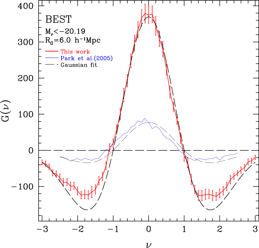
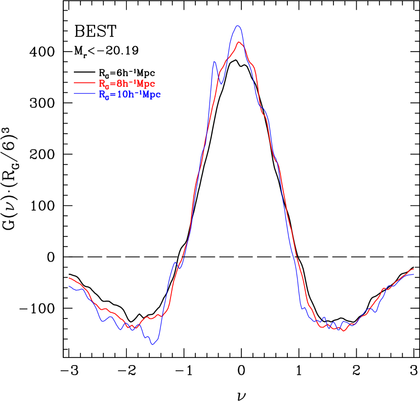
To calculate the genus a smooth density field is obtained from galaxy positions in comoving space smoothed by an $R_{G}=6.0h^{-1}$ Mpc Gaussian, $(2\pi R_{G}^{2})^{-3/2}\exp(-r^{2}/2R_{G}^{2})$ . This definition differs from that of some previous works (Hamilton et al. 1986; Park et al. 1992; Vogeley et al. 1994), which is related with current definition by $\lambda=\sqrt{2}R_{G}$ . The solid line with error bars shows measurements from the observational data, and the long-dashed line is its best-fit Gaussian curve. As a comparison, we include the results (curves with smaller amplitudes) from the BEST sample of SDSS Data Release 3 (DR3) measured by Park et al. (2005). As the DR7 sample covers the northern sky without a gap, the volume-to-surface ratio increased significantly since DR3, and the amplitude of the genus curve increased remarkably. The amplitude is now $G=373\pm 18$ with only 4.6% uncertainty, including all systematic effects and cosmic variance.

Figure 5 shows that the observed genus curve deviates from the Gaussian one in such a way that the genus at high thresholds has smaller amplitude. This means there are fewer voids and fewer superclusters when compared with the Gaussian genus curve. In other words, voids and superclusters are more connected and their sizes are larger than those expected for Gaussian fields. In addition, the positive ( $G>0$ ) region of the genus curve is slightly but systematically shifted towards lower $\nu$ values, and the percolation of large-scale structure (maximum $G$ ) occurs slightly below $\nu=0$ . According to the perturbation theory prediction of Matsubara (1994), if there were only non-linear gravitational effects involved, with no biasing, then one should find $A_{V}+A_{C}=2$ at all scales (Park et al. 2005), and the N-body results presented for dark matter in Figure 18 below are consistent with this expectation. Since the observed $A_{V}$ and $A_{C}$ are both less than $1$ , it shows that biasing effects are involved.

4.2. Mock Surveys and Systematic Biases

The genus curve in Figure 5 is affected by peculiar velocity distortions, boundary effects, and finite sampling of the density field. However, using detailed comparisons to mock catalogs from cosmological simulations, we will show that the deviations from the Gaussian field prediction, and indeed from the expected non-linear matter density field, are genuine, and statistically significant.

We use mock galaxies to estimate uncertainties in the measured genus and to measure the systematic effects due to survey boundaries, variation of angular selection function, galaxy biasing, and redshift space distortion. We adopt the halo-galaxy one-to-one correspondence (HGC) model of Kim et al. (2008) to assign mock galaxies to dark halos identified in a cosmological N-body simulation. For this purpose we made two N-body simulations of the $\Lambda$ CDM model having the WMAP 3 year cosmological parameters. The simulation and cosmological parameters adopted in the simulations (S1 and S2) are listed in Table 2.

Table 2N-body Simulation Parameters

Parameter	S1	S2
$N_{p}$ ²²2Number of CDM particles	$2048^{3}$	$2048^{3}$
$N_{m}$	$2048^{3}$	$2048^{3}$
$L_{box}$	$1024{h^{-1}\,{\rm Mpc}}$	$1433.6{h^{-1}\,{\rm Mpc}}$
$N_{step}$ ³³3Number of global evolution timesteps from $z_{i}$ to present epoch	1880	1250
$z_{i}$ ⁴⁴4Initial redshift where the simulation started	47	50
$m_{p}$ ⁵⁵5Simulation particle mass	$8.3\times 10^{9}h^{-1}M_{\odot}$	$2.3\times 10^{10}h^{-1}M_{\odot}$
$\epsilon$ ⁶⁶6Force resolution	$0.05{h^{-1}\,{\rm Mpc}}$	$0.07{h^{-1}\,{\rm Mpc}}$
$M_{h,min}$ ⁷⁷7Minimum halo mass	$2.5\times 10^{11}h^{-1}M_{\odot}$	$6.8\times 10^{11}h^{-1}M_{\odot}$
$\bar{d_{h}}$ ⁸⁸8Mean halo separation	$4.4{h^{-1}\,{\rm Mpc}}$	$5.9{h^{-1}\,{\rm Mpc}}$
$h$	0.737	0.737
$\Omega_{m}$	0.238	0.238
$\Omega_{b}$	0.042	0.042
$\Omega_{\Lambda}$	0.762	0.762
$n_{s}$	0.958	0.958
$b$	1.314	1.314

The simulations were started at the initial redshift of $z_{i}$ , and evolved to the present epoch after making $N_{step}$ global timesteps. Then dark matter particles at the present epoch are used to identify the dark halos. The CDM particles in high density regions are first found by using the Friend-of-Friend (FoF) algorithm with connection length of 0.2 times the mean particle separation, and then gravitationally bound and tidally stable dark halos are identified within each FoF particle group (Kim & Park 2006). These dark halos include isolated, central and satellite halos composing FoF halos. The halos are required to contain at least 30 particles, which corresponds to $2.5\times 10^{11}h^{-1}M_{\odot}$ for $1024{h^{-1}\,{\rm Mpc}}$ box size simulation (S1) and $6.8\times 10^{11}h^{-1}M_{\odot}$ for $1433.6{h^{-1}\,{\rm Mpc}}$ box size one (S2). The resulting halo samples include 12,326,725 and 14,244,305 dark matter halos, and the corresponding mean halo separations are $4.4{h^{-1}\,{\rm Mpc}}$ and $5.9{h^{-1}\,{\rm Mpc}}$ , respectively.

To select mock galaxies corresponding to those in BEST from the S1 simulation, we sort the dark halos in mass and choose those above a mass cut so that the resulting halo set has mean halo separation of $6.1h^{-1}$ Mpc which is the mean separation between galaxies in BEST. These halos are identified as the galaxies that can be compared with those in BEST.

We make 27 mock BEST samples originating at random locations within the S1 simulation using exactly the same survey mask, angular selection function, radial boundaries, and smoothing length, and also taking into account the peculiar velocities of the mock galaxies by adding the line of sight component of the peculiar velocity to the distance of each galaxy, and we calculate the genus curve for each sample over a set of smoothing lengths. We do not enforce non-overlapping volumes for these mock samples, but the ratio of the simulation volume to the BEST sample volume is approximately 40:1, so the 27 mock catalogs are approximately independent. The error bars in Figure 5 are the standard deviation of the genus curves from these 27 mock surveys. The derived statistics such as the amplitude ( $g$ ), shift ( $\Delta\nu$ ), cluster abundance ( $A_{C}$ ), and void abundance ( $A_{V}$ ) parameters are then measured from the genus curves.

The genus calculated from the observational data suffers from systematic effects due to redshift space distortion and complicated survey boundaries. To estimate the effects we use the difference between the genus curves measured from the real-space galaxy distribution in the whole simulation cube and from the redshift-space galaxy distribution in the mock surveys. For example, we measure the genus density ${g_{r}}^{\rm cube}$ at a smoothing scale $R_{G}$ using all halos with mass $M_{h}>7.9\times 10^{11}h^{-1}M_{\odot}$ ( $\bar{d}=6.1h^{-1}$ Mpc) in the simulation cube. Halo positions in real space are used for ${g_{r}}^{\rm cube}$ . The mean genus density ${g_{z}}^{\rm mock}$ is also calculated from the 27 mock SDSS surveys where the halos with $M_{h}>7.9\times 10^{11}h^{-1}M_{\odot}$ are observed in the simulation, with their redshift space positions. The difference between the two contains the information on the systematic effects of survey boundaries and redshift-space distortion (RSD). The observed genus in real space can be estimated by ${g_{r}}^{\rm obs}={g_{z}}^{\rm obs}{g_{r}}^{\rm cube}/{g_{z}}^{\rm mock}$ assuming that the correction is model-insensitive. The correction factor is obtained from the ratio of the two statistics in the case of $g,A{{}_{C}}$ , and $A_{V}$ , and from the difference in the case of $\Delta\nu$ .

The correction is expensive because we need to find the correction factors for all statistics whenever we change the volume-limited sample or the smoothing scale. But there is a big advantage for presenting the observational data corrected for the survey boundary effects and RSD effects. It enables one to compare the observational data with theoretical predictions based on analytic calculations or the analysis of the simulation data without taking into account the particular survey characteristics. An empirical study on the systematic effects on the genus is presented in Appendix A.

4.3. Scale-dependent Topology Bias

Table 3Genus-Related Statistics of the Scale-Dependence Samples in Figure 6

Statistics	$R_{G}$
	6.0	7.0	8.0	9.0	10.0
$G$	$410.0(373.8)\pm 17.9$	$270.3(247.0)\pm 13.5$	$184.7(168.1)\pm 10.6$	$133.7(121.8)\pm 9.3$	$97.5(89.4)\pm 7.3$
$\Delta\nu$	$-0.023(-0.027)\pm 0.019$	$-0.027(-0.027)\pm 0.024$	$-0.047(-0.045)\pm 0.030$	$-0.068(-0.063)\pm 0.033$	$-0.072(-0.066)\pm 0.036$
$A_{V}$	$0.70(0.71)\pm 0.04$	$0.73(0.74)\pm 0.05$	$0.77(0.78)\pm 0.06$	$0.76(0.77)\pm 0.06$	$0.81(0.81)\pm 0.07$
$A_{C}$	$0.83(0.81)\pm 0.05$	$0.84(0.83)\pm 0.07$	$0.85(0.84)\pm 0.08$	$0.84(0.83)\pm 0.08$	$0.81(0.80)\pm 0.07$

Note. $R_{G}$ is the smoothing length in units of ${h^{-1}\,{\rm Mpc}}$ . G is the amplitude of the genus curve, $\Delta\nu$ is the shift parameter, and $A_{C}$ and $A_{V}$ are cluster and void abundance parameters, respectively. All these values are systematic bias-corrected, and the observed values before the systematic bias corrections are given in parentheses. Uncertainty limits are estimated from 27 mock surveys in redshift space.

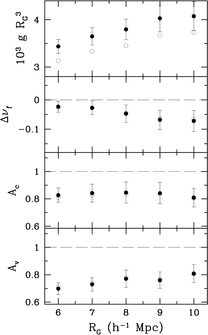
To study the scale dependence of topology without the effects of changing large-scale structure in the survey volume, we fix the sample definition (i.e. angular and radial boundaries) and change the smoothing length only. Figure 6 shows the genus-related statistics (filled circles with error bars) as a function of Gaussian smoothing length in the case of the BEST sample and the data are given in Table 3. Error bars are obtained from 27 mock BEST surveys made in the S1 $\Lambda$ CDM simulation using the halos having the mean separation of $6.1h^{-1}$ Mpc. Open circles are the statistics before the systematic bias corrections are made.

Figure 6 demonstrates that the deviation from the Gaussian-field topology is scale-dependent. The second panel shows that genus curve shifts towards increasingly negative values of $\Delta\nu$ (“meatball” topology) as $R_{G}$ increases from 6 to $10h^{-1}\,$ Mpc. The fractionally largest and statistically strongest deviations from the Gaussian field prediction arise for the void abundance parameter $A_{V}$ , which rises from 0.7 at $6{h^{-1}\,{\rm Mpc}}$ to 0.8 at $10{h^{-1}\,{\rm Mpc}}$ (compared to $A_{V}=1$ ). We call these phenomena the scale-dependence of galaxy clustering topology. The cluster abundance $A_{C}$ also differs from the Gaussian-field prediction $A_{C}=1$ , but in a way that is approximately constant with smoothing length over this range. Note that the figures plot $gR{{}_{G}}^{3}=(G_{\rm obs}/V_{sample})R{{}_{G}}^{3}$ , which is proportional to the genus per unit smoothing volume.

To visually relate these measures to genus curve shapes, we show the genus curves for $R{{}_{G}}=6,8$ , and $10h^{-1}\,$ Mpc, scaled by $(R{{}_{G}}/6h^{-1}{\rm Mpc})^{3}$ in Figure 7.

To understand the bias in the topology of galaxy clustering we need to know the underlying matter field. We assume the matter field of the universe is equal to that of our $\Lambda$ CDM simulation with WMAP 3 year parameters. The genus is calculated for the CDM field (of the full $1024{h^{-1}\,{\rm Mpc}}$ simulation cube) as in Figures 1 and 2 of Park, Kim & Gott (2005) and compared to that of the observed genus in Figure 8 where deviations of $g_{g}/g_{m},A_{C,g}/A_{C,m}$ , and $A_{V,g}/A_{V,m}$ from 1, or deviation of $\Delta\nu_{g}-\Delta\nu_{m}$ from 0 indicate the galaxy biasing with respect to matter. We find significant bias in the topology of the galaxy distribution for all four statistics. When compared to the matter distribution, galaxy clustering shows more complicated structures (higher $g$ ), has more meat-ball shifted topology (more negative $\Delta\nu$ ), fewer number of superclusters (smaller $A_{C}$ ), and fewer number of voids (smaller $A_{V}$ ). In particular, the void abundance shows a very strong bias which has a strong scale-dependence. Any successful galaxy formation model should explain this topology bias in the distribution of galaxies.

James et al. (2007, 2009) studied the scale dependence of topology using the 2dFGRS samples. James et al. (2009) measured the genus statistic as a function of scale from 5 to $8{h^{-1}\,{\rm Mpc}}$ , using analytic predictions for both the linear regime (Gaussian random field) and weakly non-linear regime (perturbation theory; Matsubara 1994; Matsubara & Suto 1996) to detect the effects of non-linear structure formation on the genus statistic, and found that both $A_{V}$ and $A_{C}$ tend to fall below unity independently of scale and that neither of the analytic prescriptions satisfactorily reproduces the measurement.

Quantitative meausures of the shape parameters of the genus curve before and after the bias correction shown in Figure 6 help us understand the degree of the RSD effects on the genus. We find that the survey boundary effects are very small because the volume-to-surface ratio is quite large for the SDSS DR7 data (see blue solid and black dashed lines in the top panel of Figure 18 in Appendix A).

On $6{h^{-1}\,{\rm Mpc}}$ smoothing scale the shape parameters ( $\Delta\nu$ , $A_{C}$ , and $A_{V}$ ) change only a little while the amplitude reduction is as much as $8.8$ %. The RSD effects make the $\nu>1$ part of the genus curve ( $A_{C}$ ) have an amplitude lowered by $2.4\%$ , and increase the $\nu<-1$ part ( $A_{V}$ ) by $1.4\%$ relative to the best-fitting Gaussian genus curve (see Table 3). Even though the overall amplitude of the genus curve is rather sensitive to the RSD effects, its shape is not. This fact is in agreement with the perturbative theoretical description of Matsubara & Suto (1996).

To compare Matsubara (1996)’s linear prediction for the RSD effects with those calculated from simulation, we measure the amplitude of the genus curves of the 27 mock survey samples both in redshift space and real space, which are denoted by $G^{z}(\nu)$ and $G^{r}(\nu)$ , respectively. Their ratios are plotted as a function of the smoothing length in Figure 9.

Dashed line is the linear theory prediction according to Matsubara (1996)

\frac{G^{z}(\nu)}{G^{r}(\nu)}=\frac{3\sqrt{3}}{2}\sqrt{u}(1-u),\\

(6)

where

u=\frac{1}{3}\frac{1+(6/5)fb^{-1}+(3/7)(fb^{-1})^{2}}{1+(2/3)fb^{-1}+(1/5)(fb^{-1})^{2}}.

(7)

The $b$ is the bias parameter and the function $f$ is given by

f(\Omega_{m},\Omega_{\lambda})\equiv d{\rm ln}D/d{\rm ln}a\approx\Omega_{m}^{0.6}+\frac{\Omega_{\lambda}}{70}(1+\frac{\Omega_{m}}{2})

(8)

where $D(t)$ is the linear growth factor and $a$ is the scale factor. The linear theory predicts $G^{z}(\nu)/G^{r}(\nu)=0.991$ , while our result is 0.931 at $R_{G}=6{h^{-1}\,{\rm Mpc}}$ . $G^{z}(\nu)/G^{r}(\nu)$ tends to slowly approach the linear prediction as the smoothing length increases. Matubara & Suto (1996) have pointed out that in weakly non-linear regimes the RSD tends to suppress the amplitude more strongly than the linear theory prediction, in agreement with our result. Figure 9 also shows that, apart from the sample-to-sample fluctuation in the observed density field, the sample-to-sample variation in the large-scale peculiar velocity field causes about 1.5% uncertainty in the RSD correction on the $R_{G}=6{h^{-1}\,{\rm Mpc}}$ scale in the case of the SDSS DR7 sample. (Note that Fig. 9 shows the effects of RSD only with the density field in each sample fixed.)

4.4. Dependence of Topology on Galaxy Properties

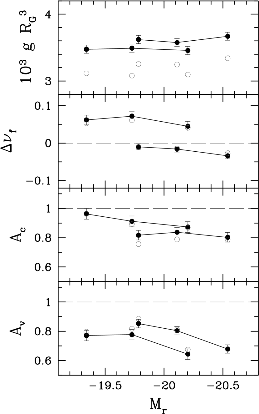
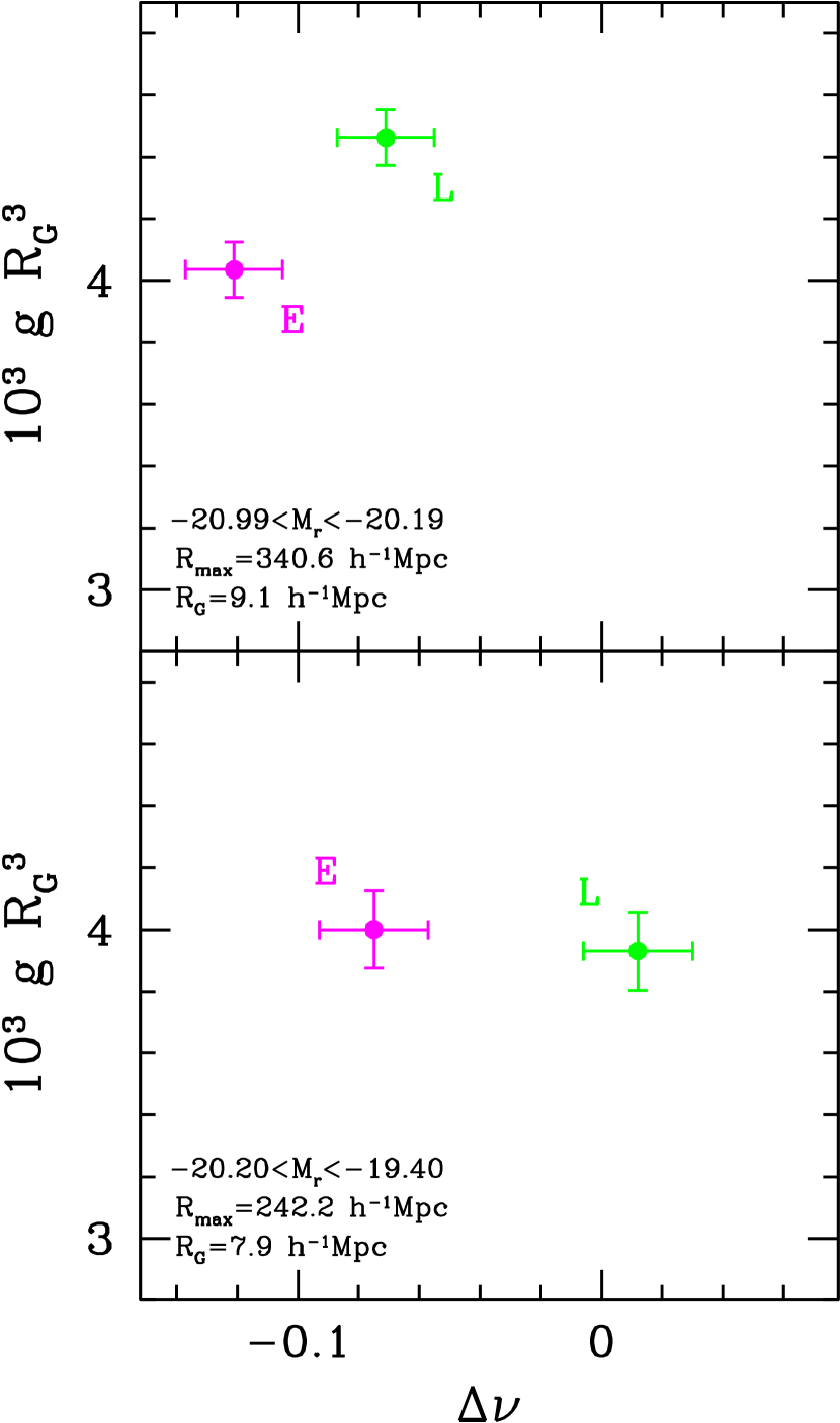
Park et al. (2005) presented the first clear demonstration of luminosity dependence of galaxy clustering topology: brighter galaxies show a stronger signal of “meatball” topology. To quantify the luminosity bias we use two volume-limited samples with $-19.0>M_{r}>-21.0$ (corresponding to a comoving distance range of $59.7<R<203.2{h^{-1}\,{\rm Mpc}}$ ) and $-19.5>M_{r}>-21.5$ ( $59.7<R<253.0{h^{-1}\,{\rm Mpc}}$ ). Each sample is divided into three subsets of galaxies belonging to three absolute magnitude ranges. To be free from confusion due to changing levels of discrete sampling of structures (random fluctuations in the number of galaxies that trace the density field), we choose the subsamples to contain the same number of galaxies. Since each of the three subsets includes the same number of galaxies distributed in the same volume of the universe, any difference in topology must be due to difference in luminosity. We then measure the genus-related statistics to quantify the luminosity bias. The statistics measured for $R_{G}=5.9h^{-1}$ Mpc are plotted in Figure 10. The scale is chosen because it is the mean separation of the galaxies in the subsets of the bright volume-limited sample. This smoothing length is also used for the subsets of the faint sample, whose $\bar{d}$ is $5.4{h^{-1}\,{\rm Mpc}}$ . The $x$ -coordinate of each filled circle is the median absolute magnitude of each subset, and three circles corresponding to three subsets of the same volume-limited sample are connected together.

In Figure 10 there are two sets of connected points corresponding to the two volume-limited samples. Differences between the two sets are due to the fact that the samples enclose the universe with different outer boundaries (i.e., cosmic variance) and should not be paid attention here. The luminosity dependence of topology appears within each volume-limited sample.

To estimate the significance of the luminosity bias we make 20 mock subsets for each volume-limited sample by selecting $1/3$ of the galaxies randomly without taking into account luminosity. Observational and mock subsets have the same sample volume, geometry, and galaxy number density. They differ only by galaxy luminosity. We use those mock subsets to estimate the error bars in Figure 10. Therefore, they do not contain the cosmic variance, and show the significance of luminosity selection only.

It can be seen that the distribution of brighter galaxies tends to have a stronger “meatball” topology signature (more negative $\Delta\nu$ ) and greater percolation of underdense regions (lower $A_{V}$ ). But the luminosity dependence for the shift ( $\Delta\nu$ ) parameter is somewhat mild, particularly for the faint sample. We do not detect any statistically significant dependence of $g$ on luminosity.

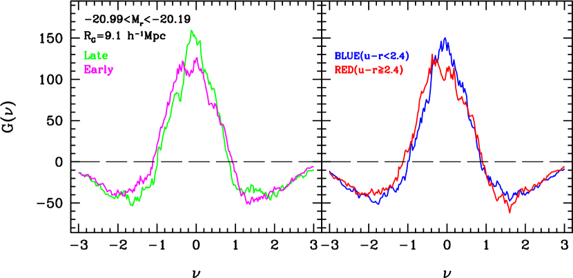
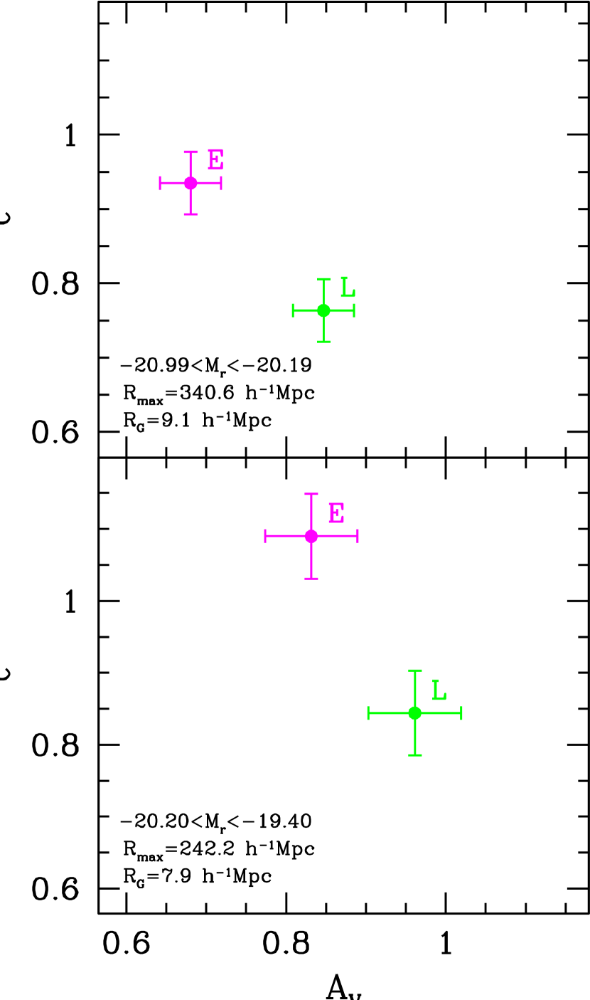
After luminosity we consider morphology. It is well-known that early-type galaxies are dominant in massive clusters and late types are abundant in the field, and one naturally expects morphology dependence of the topology of galaxy clustering. The left panel of Figure 11 shows the genus curves of early- (red curve with a smaller amplitude) and late-type galaxies with $-20.99<M_{r}<-20.19$ at 9.1 $h^{-1}$ Mpc Gaussian smoothing scale. We limit the absolute magnitude range to reduce the luminosity-dependent bias and to inspect the morphology dependence of the genus only.

We find the mean galaxy separations of the early- and late-type galaxy samples are 8.9 and 8.3 $h^{-1}$ Mpc, respectively. We discard the most edge-on late-type galaxies to make the mean galaxy separation in the late-type sample equal to 8.9 $h^{-1}$ Mpc. In Table 4, $\bar{d}$ before the thinning out is given in parentheses. The smoothing length of $R_{G}=9.1h^{-1}$ Mpc is chosen because it is the mean separation of ‘blue’-type galaxies, which we will use below to study the difference between morphology and color dependence. The systematic effects are again corrected and error bars are estimated from 20 subsets drawn out of the volume-limited sample made by selecting galaxies randomly without considering morphology. Each set has the mean galaxy separation of $\bar{d}=8.9h^{-1}$ Mpc. It can be easily seen that the genus curve for early-type galaxies has a smaller overall amplitude, fewer voids, and more clusters, and is meat-ball shifted compared to that of late-type galaxies. These differences are manifest in Figure 12 where we show the genus-related parameters for early- and late-type samples separately.

Table 4Genus-related Statistics of the Morphology-Dependence Samples in Figure 12

	$-20.19>M_{r}>-20.99$		$-19.40>M_{r}>-20.20$
	$(59.7<R<340.6{h^{-1}\,{\rm Mpc}})$		( $59.7<R<242.2{h^{-1}\,{\rm Mpc}}$ )
	Early	Late	Early	Late
Statistics	$\bar{d}=8.9$	$\bar{d}=8.9(8.3)$	$\bar{d}=7.9$	$\bar{d}=7.9(6.3)$
$G$	$128.1(117.4)\pm 2.9$	$141.7(129.8)\pm 2.9$	$66.6(61.2)\pm 2.1$	$65.4(60.1)\pm 2.1$
$\Delta\nu$	$-0.121(-0.111)\pm 0.028$	$-0.071(-0.061)\pm 0.028$	$-0.075(-0.067)\pm 0.018$	$0.012(0.020)\pm 0.018$
$A_{V}$	$0.68(0.67)\pm 0.04$	$0.85(0.84)\pm 0.04$	$0.83(0.85)\pm 0.06$	$0.96(0.99)\pm 0.06$
$A_{C}$	$0.93(0.91)\pm 0.04$	$0.76(0.74)\pm 0.04$	$1.09(1.03)\pm 0.06$	$0.84(0.80)\pm 0.06$

Note. $\bar{d}$ is the mean galaxy separation in units of ${h^{-1}\,{\rm Mpc}}$ . $\bar{d}$ in parentheses is the value before the thinning out the late-type sample. All genus-related statistics are systematic bias-corrected, and the observed values before the correction are given in parentheses.

The upper panels are for the brighter sample mentioned above, and the lower panels are for relatively fainter galaxies with $-20.20<M_{r}<-19.40$ . In the lower panels, the smoothing length $R_{G}$ is 7.9 $h^{-1}$ Mpc, which corresponds to the mean separation of the early-type galaxies with magnitudes in this range (see Table 12). Table 9 in Appendix C gives the data for the genus curves. Table 4 lists the measured genus-related statistics, both corrected and uncorrected (in parentheses) for systematics. It is evident that significant morphology bias in the topology of the galaxy distribution exists, confirming the difference between the early- and late-type distributions predicted from hydrodynamic cosmological simulations by Gott, Cen, & Ostriker (1996).

Next, we examine whether the genus curve depends on galaxy color or not. Although the morphology and color are strongly correlated with each other, the roles of morphology and color in galaxy evolution are expected to be different. For example, galaxy color seems to depend mainly on the distance and morphology of the nearest neighbor galaxy, while morphology depends not only on neighbor but also on the distance to the nearest massive cluster of galaxies (Park & Hwang 2009). Thus, it is interesting to examine separately how the galaxy clustering topology depends on these two physical parameters.

For the color comparison, the genus curves of red ( $u-r\geq 2.4$ ) and blue ( $u-r<2.4$ ) galaxies with $-20.99<M_{r}<-20.19$ are plotted in the right panel of Figure 11. We create red and blue samples with the same number of galaxies by randomly throwing away some galaxies in the larger sample. Edge-on galaxies are discarded here. In Table 7 of Section 5.3, the mean separation of galaxies in each sample and smoothing length are given. In this color-dependence analysis, we adopted the same sample used for the morphology-dependence study. The genus-related statistics for the color subsamples are shown in Figure 13 together with those of morphology samples for comparison. Table 9 in Appendix C gives the data for the genus curves, and Table 8 in Section 5.3 lists all the measured genus-related parameters.

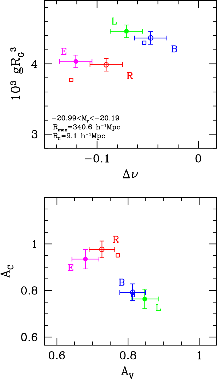
Similarly to the early-type galaxies, the distribution of red galaxies has a smaller overall amplitude of the genus curve, fewer voids, and more clusters, and is meat-ball shifted compared to that of blue galaxies. The result confirms the relative meatball shift between red and blue galaxies detected in a 2-D topology survey from the SDSS Early Data Release by Hoyle et al. (2002).

There is one major difference between topology of morphology subsets and color subsets. The contrast in $A_{V}$ between the early and late subsets is much larger than that between red and blue subsets. This can be also seen for fainter galaxies with $-20.20<M_{r}<-19.40$ used in Section 5.3. The dependence of the void abundance on color is much reduced, while the dependence on morphology still exists in the fainter magnitudes as shown in the bottom right panel of Figure 12.

5. Test of Galaxy Formation Models

5.1. Galaxy Formation Models

Galaxies are the end product of non-linear gravitational evolution of primordial density fluctuations. Therefore, the spatial distribution of galaxies and its dependence on the internal properties of galaxies should depend both on initial conditions and on galaxy formation and evolution processes. This enables us to test galaxy formation models as well as the models on primordial fluctuations using topology. In this section we examine whether or not various models of galaxy formation are consistent with our measurement of topology of galaxy clustering, assuming that the difference between observation and models is entirely due to inaccuracy in the galaxy formation mechanism. This assumption is supported by the fact that the topology of the Luminous Red Galaxies in the SDSS analyzed by Gott et al. (2009) agrees very well with that of the mock galaxies identified in the $\Lambda$ CDM model with the same cosmological parameters (i.e. 3 year WMAP parameters) we adopt in this paper. Gott et al. measured the topology at very large scales of $R_{G}=21$ and $34h^{-1}$ Mpc. In this almost linear regime, the results are sensitive only to the adopted cosmological parameters. They use our simple HGC model to locate the mock LRGs in a large $\Lambda$ CDM simulation. Gott et al.’s results indicate that our cosmological model, which adopts the initially Gaussian primordial fluctuations with the WMAP 3 year $\Lambda$ CDM power spectrum, is consistent with the observation in the linear regime. If one finds a discrepancy between observation and models in the galaxy clustering topology on non-linear scales, therefore, it most likely arises from inaccuracy in the galaxy formation models.

We adopt five galaxy allocation schemes applied to cosmological N-body simulations. The first is the HGC model described in Section 4.2. Each of the dark halos identified in our S1 $\Lambda$ CDM simulation of 2048³ CDM particles in a 1024 $h^{-1}$ Mpc size box is assumed to host one galaxy. The halos used in the HGC model can be either isolated or grouped, and in the latter case they can be the central one or satellites. The second is a Halo Occupation Distribution (HOD) model of Yang et al. (2007) refined by introducing a conditional luminosity function (van den Bosch et al. 2007) that accurately matches the SDSS luminosity function and the clustering properties of SDSS galaxies as a function of their luminosity. The other three models that we examine are different implementations of semi-analytic models of galaxy formation (SAMs): Croton et al. (2006), Bower et al. (2006), and Bertone et al. (2007). All of them are set in the context of structure formation in a CDM universe as modelled by Millennium Simulation (Springel et al. 2005) of 2160³ particles in a 500 $h^{-1}$ Mpc size box ( $\Omega_{m}=0.25,\Omega_{\Lambda}=0.75,\Omega_{b}=0.045,h=0.73,n{{}_{s}}=1$ were assumed). However, they used different construction of the dark matter merger trees and different implementation of the various physical processes involving the baryonic component of the universe. Croton et al. and Bower et al. invoked ‘radio-mode’ AGN feedback schemes to restrict gas cooling within relatively massive halos. The prescriptions in both models were set by the requirement that they approximately reproduce the observed break in the present day luminosity function at bright magnitudes, but their detailed implementations differ. Bertone et al. have used a variation of the SAM of de Lucia & Blaizot (2007), which is the later version of the galaxy formation models described in Croton et al., and implemented supernova feedback using a ‘dynamical’ treatment of galactic winds (Bertone, Stoehr & White 2005). The treatment of fast recycling of ejected gas and metals predicts a relatively low abundance of dwarf galaxies in better agreement with observations but a rather larger number of bright galaxies than observed.

5.2. Topology Test

For a given luminosity cut of a volume-limited sample of the SDSS galaxies, the mean galaxy separation $\bar{d}$ and the maximum sample depth are determined. To compare the mock galaxies generated by the above five galaxy formation models in a fair way, we set the mean separation between the mock galaxies in each model equal to the observed value by adjusting the lower limit of galaxy mass or luminosity. This gives us the relation between $\bar{d}$ and the limiting absolute magnitude $M_{r,\rm cut}$ . The outer boundary $R_{\rm max}$ of the volume-limited sample is determined for the apparent magnitude limit of $r=17.6$ and the absolute magnitude limit of $M_{r,\rm cut}$ .

Comparisons among the observations and models are made for galaxies with the same number density or $\bar{d}$ . For example, we sort all galaxies (halos) in our HGC catalog and find the mass cut above which the mean galaxy separation is equal to that of each volume-limited sample of the SDSS galaxies. The resulting sample of mock galaxies with mass above the cut is to be compared with the corresponding observational sample. Mock galaxy subsets are similarly made for the HOD and three SAM galaxy samples. The mass or luminosity cuts are given in Table 5.

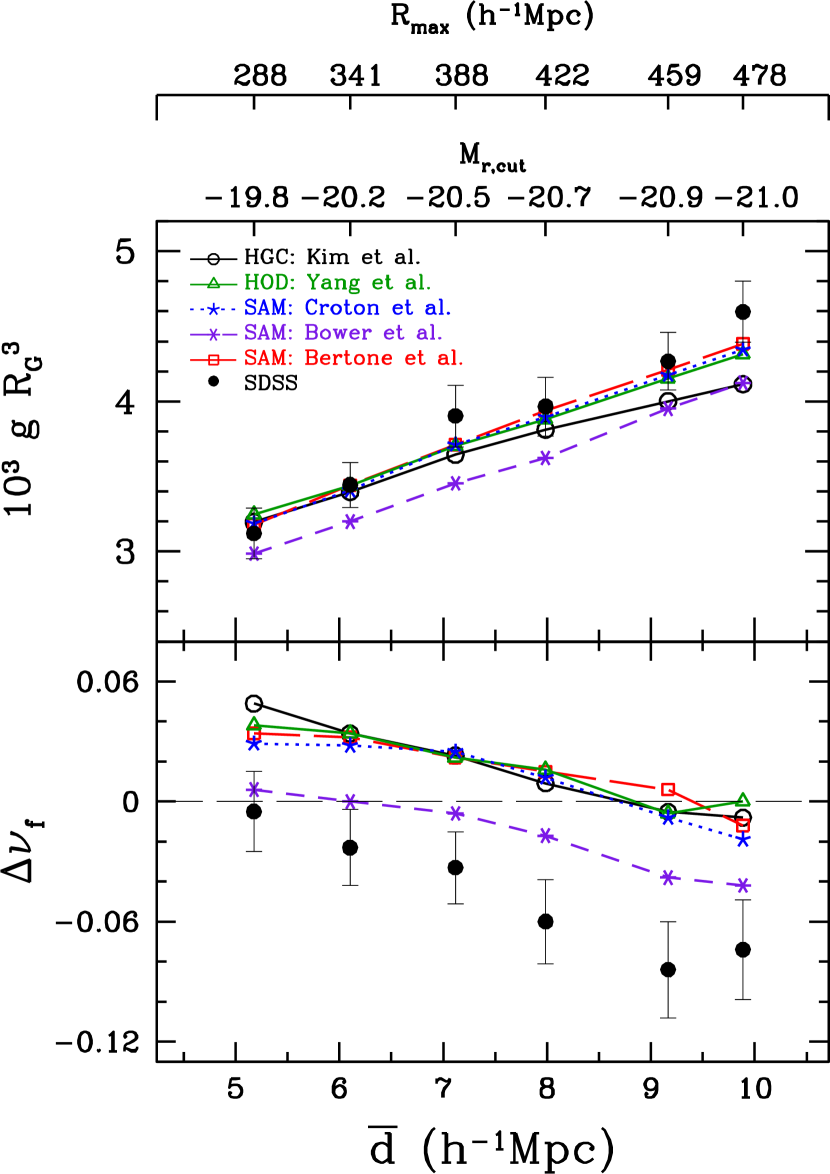
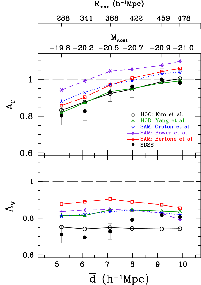
The genus-related statistics measured from six volume-limited samples of the SDSS galaxies (dots with error bars) are plotted in Figure 14 at locations corresponding to the sample defining parameters ( $\bar{d}$ , $M_{r,\rm cut}$ , $R_{\rm max}$ ) which are also given in Table 5. It should be noted that the observed volume-limited sample contains progressively brighter galaxies and the sample depth $R_{\rm max}$ increases as the mean galaxy separation $\bar{d}$ increases. Figure 14 also shows the results for the mock galaxies of five galaxy formation models. Table 6 lists the statistics for all models and samples.

Table 5Sample Defining Parameters of six volume-limited samples used in Figure 14

$R_{\rm G}$	$\bar{d}$	$R_{\rm min},R_{\rm max}$	$M_{r,\rm cut}^{\rm SDSS}$	$M_{\rm cut}^{\rm HGC}$	$M_{r,\rm cut}^{\rm HOD}$	$M_{r,\rm cut}^{\rm Croton}$	$M_{r,\rm cut}^{\rm Bower}$	$M_{r,\rm cut}^{\rm Bertone}$
5.2	5.17	59.7, 288.1	$-19.80$	11.67	$-19.86$	$-20.08$	$-20.36$	$-21.25$
6.0	6.10	59.7, 340.6	$-20.19$	11.90	$-20.26$	$-20.46$	$-20.72$	$-21.62$
7.2	7.11	59.7, 388.3	$-20.50$	12.10	$-20.56$	$-20.75$	$-21.00$	$-21.87$
8.0	7.99	59.7, 422.2	$-20.70$	12.25	$-20.74$	$-20.94$	$-21.20$	$-22.03$
9.2	9.17	59.7, 458.6	$-20.90$	12.43	$-20.94$	$-21.13$	$-21.42$	$-22.21$
9.9	9.89	59.7, 477.8	$-21.00$	12.52	$-21.04$	$-21.23$	$-21.53$	$-22.30$

Note. – Cols.(1) Gaussian smoothing length in units of ${h^{-1}\,{\rm Mpc}}$ ; (2) Galaxy mean separation in units of ${h^{-1}\,{\rm Mpc}}$ ; (3) Inner and outer boundary of the SDSS volume-limited samples in units of ${h^{-1}\,{\rm Mpc}}$ ; (4) Absolute $r$ -band magnitude at $z=0.1$ of the SDSS sample ( $K$ and evolution corrected); (5) Logarithmic mass cut of halos in HGC model sample in units of $h^{-1}M_{\odot}$ ; (6) Absolute $r$ -band magnitude at $z=0.1$ ( $K$ and evolution corrected) of the HOD galaxy sample; (7), (8) and (9) Absolute rest frame $r$ -band magnitude cuts of three SAM galaxy samples.

Table 6Genus-related Statistics for the samples used in Figure 14

Statistics	$R_{\rm G}$	SDSS	HGC	HOD	SAM^Croton	SAM^Bower	SAM^Bertone
$G$	5.2	$343.5(312.7)\pm 18.5$	352.0	357.6	350.9	328.9	349.9
	6.0	$410.0(373.8)\pm 17.9$	404.6	409.4	405.8	380.9	409.8
	7.2	$397.2(363.9)\pm 20.9$	371.0	377.0	377.8	351.6	377.9
	8.0	$377.9(348.9)\pm 18.6$	363.4	369.6	371.3	345.1	375.1
	9.2	$340.8(317.9)\pm 15.3$	319.4	331.6	333.4	315.6	336.2
	9.9	$331.7(308.8)\pm 14.7$	297.0	311.2	313.5	297.7	316.5
$\Delta\nu$	5.2	$-0.005(-0.011)\pm 0.020$	0.049	0.038	0.029	0.006	0.034
	6.0	$-0.023(-0.027)\pm 0.019$	0.034	0.034	0.028	0.000	0.032
	7.2	$-0.033(-0.030)\pm 0.018$	0.023	0.022	0.025	-0.006	0.022
	8.0	$-0.060(-0.057)\pm 0.021$	0.009	0.016	0.012	-0.017	0.015
	9.2	$-0.084(-0.075)\pm 0.024$	-0.005	-0.006	-0.008	-0.038	0.006
	9.9	$-0.074(-0.069)\pm 0.025$	-0.008	0.000	-0.019	-0.042	-0.012
$A_{V}$	5.2	$0.71(0.73)\pm 0.05$	0.75	0.81	0.81	0.84	0.88
	6.0	$0.70(0.71)\pm 0.04$	0.74	0.81	0.82	0.84	0.89
	7.2	$0.73(0.75)\pm 0.04$	0.75	0.84	0.83	0.85	0.91
	8.0	$0.79(0.81)\pm 0.04$	0.74	0.84	0.84	0.84	0.89
	9.2	$0.82(0.84)\pm 0.05$	0.74	0.84	0.83	0.83	0.87
	9.9	$0.81(0.82)\pm 0.05$	0.74	0.83	0.82	0.79	0.85
$A_{C}$	5.2	$0.80(0.79)\pm 0.05$	0.83	0.82	0.88	0.94	0.86
	6.0	$0.83(0.81)\pm 0.05$	0.88	0.87	0.93	0.99	0.90
	7.2	$0.93(0.91)\pm 0.05$	0.92	0.93	0.97	1.04	0.97
	8.0	$0.96(0.95)\pm 0.06$	0.95	0.95	0.99	1.05	1.01
	9.2	$1.00(0.98)\pm 0.06$	0.99	0.98	1.03	1.08	1.04
	9.9	$0.98(0.97)\pm 0.07$	1.00	0.99	1.04	1.10	1.06

Note. Systematic corrected parameters Genus-related statistics measured from six volume-limited SDSS samples and from mock galaxy samples of five galaxy formation models. The smoothing length $R_{G}$ is in units of $h^{-1}$ Mpc. The observed values are corrected for the systematic biases, and those before the correction are given in parentheses.

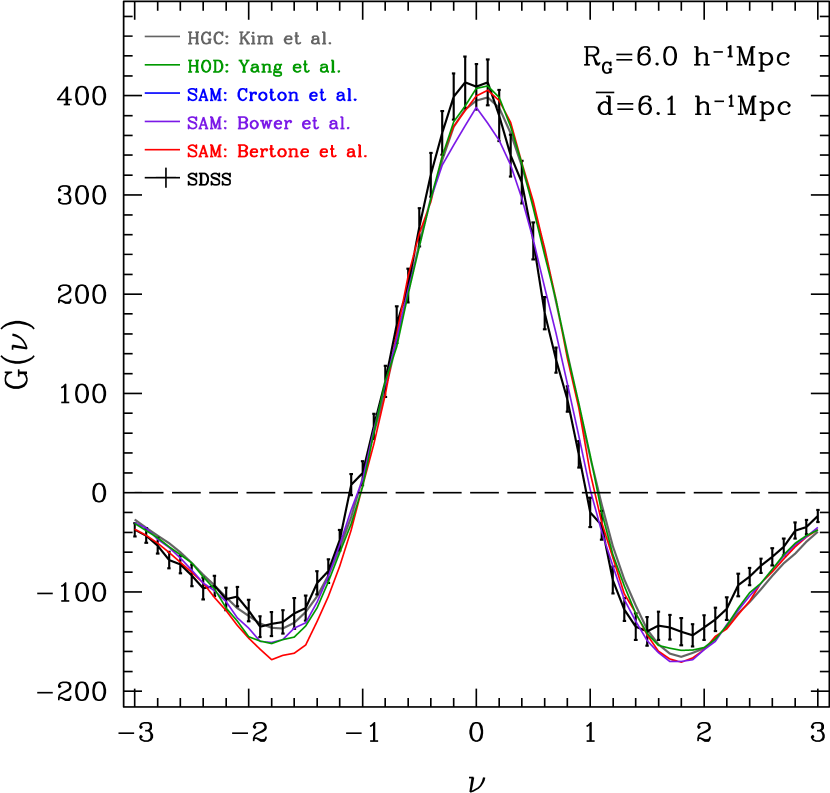
Figure 15 shows the genus curves for the SDSS galaxies in the BEST sample and for the five sets of mock galaxies with 6.0 $h^{-1}$ Mpc smoothing. Table 10 in Appendix C gives genus curves of the SDSS and mock galaxies. Four models, the exception being Bower et al. (2006), agree very well with one another for the genus density and shift parameters over the scales explored. Those four models agree well with the observations in terms of $g$ , but Bower et al. (2006) agrees better for $\Delta\nu$ . The models give diverse results for the cluster and void abundance parameters, though all of them predict $A_{V}+A_{C}<2$ at all scales shown, indicating (Matsubara 1994) that effects beyond those of perturbative non-linear gravitational evolution must be involved. Bower et al. (2006) is again most discrepant with the observation in terms of $A_{C}$ , while HGC and HOD match the observed values almost perfectly. When $A_{V}$ is considered, HOD and all SAM models are inconsistent with the observations, while HGC is within the cosmic variance from the observation. Overall, no model reproduces all features of the observed topology. Only the Bower et al. (2006) SAM comes close to matching $\Delta\nu$ , but it fares worst with $A_{C}$ and the genus density. Only HGC matches $A_{V}$ , but it fails for $\Delta\nu$ .

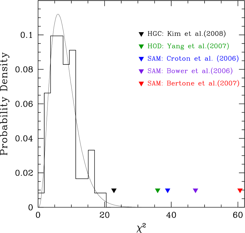
To estimate the statistical significance of the failure of each model we select two volume-limited samples with ${\bar{d}}=6.10$ and $7.11{h^{-1}\,{\rm Mpc}}$ . We calculate the $\chi^{2}$ statistic

\chi^{2}=\sum_{ij}(v_{ij}^{\rm model}-v_{ij}^{\rm obs})^{2}/\sigma_{ij}^{2},

where the index $i$ runs over the four genus-related statistics and $j$ runs over the two volume-limited samples. $\sigma_{ij}^{2}$ is the variance of the $i$ -th statistic calculated from 27 mock surveys of the $j$ -th volume-limited sample made in the S1 simulation. A distribution of this $\chi^{2}$ statistic is obtained from 64 mock volume-limited samples of the HGC galaxies made from the S2 simulation (see the histogram in Figure 16), where $v_{ij}^{\rm obs}$ is replaced by the average value over the 64 mock samples. At each of the 64 locations in the simulation two mock SDSS samples are made with depths of 340.6 and 388.3 $h^{-1}$ Mpc and with mass cuts of $10^{11.90}$ and $10^{12.10}h^{-1}M_{\odot}$ , respectively. Smoothing lengths of $R_{G}=6.0$ and $7.2{h^{-1}\,{\rm Mpc}}$ are applied to these two mock samples, respectively.

The histogram of $\chi^{2}$ computed from the mock catalogs in this way is well described by a $\chi^{2}$ distribution with 8 degrees of freedom, as expected if the errors in the four statistics at the two smoothing lengths are essentially uncorrelated. (Compare the histogram and dotted curve in Figure 16, and see further discussion in Appendix B) Assuming this distribution and applying a 1-tailed $\chi^{2}$ test, the probability for the HGC model to be consistent with the observation is only 0.4%. The HOD and three SAM models are absolutely ruled out by this test, confirming that the discrepancies seen in Figure 14 are of high statistical significance. The least inconsistent model is HGC, followed by the HOD model, while the three SAM models are the most inconsistent. These discrepancies confirm the findings of Gott et al. (2008), using the DR3 topology measurement and several N-body and hydrodynamic simulations, that existing galaxy formation models do not reproduce the topology of the SDSS main galaxy sample near the smoothing scales we are exploring. It is interesting to note that the HGC performs best among the five galaxy formation models even though it is constrained by only one observational parameter, the mean galaxy number density.

On the other hand, Gott, Choi, & Park (2009) found that the topology of the luminous red galaxies (LRGs) is successfully fit by the HGC model we have tested here, which means that for the most massive galaxies, the HGC model does seem to work well. Thus the formation of the most massive LRGs seems to be a cleaner problem that can be modeled with CDM simulations and sub-halo finding routines like those described by Kim & Park (2006).

There are several implications that can be obtained from this test on how to fix these galaxy formation prescriptions to make them reproduce the observed galaxy clustering topology. The SAM models and HOD model should be modified so that the mock galaxies do not separate voids — connecting low density regions would lower $A_{V}$ . The SAM models should also produce more connected massive clusters (i.e. smaller $A_{C}$ ). All models should produce large-scale structure percolating at lower density levels (i.e. more negative $\Delta\nu$ ). The problems with the SAM models might be alleviated if the threshold interval for galaxy formation were more narrow (i.e., fewer galaxies in low mass halos), making voids cleaner and superclusters denser.

In principle, of course, the discrepancies in Figure 15 could be a sign of non-Gaussian initial conditions, or of a linear power spectrum very different from the one we have adopted based on WMAP3. However, given that different galaxy formation prescriptions produce differences comparable in magnitude to the observed discrepancies, even though no one model matches all aspects of the observed topology, we are inclined to ascribe these discrepancies to imperfect galaxy formation physics. The dependence of topology on galaxy morphology and color also supports this interpretation, as the differences between the topology of early- and late-type galaxy subsets are larger than the discrepancies between the full galaxy sample and the observations.

5.3. Topology Test for Color Subsets

The SAM models give not only luminosity but also color of mock galaxies, which makes it possible to compare the observation and SAM models using the samples divided by color. We adjust the lower limit of galaxy luminosity to make the mean galaxy separation $\bar{d}$ equal to that of the SDSS galaxies in the volume-limited samples with $-20.2<M_{r}<-19.4$ (Sample L2) and $-20.99<M_{r}<-20.19$ (Sample L1). Then each sample is divided into red and blue subsets using a color cut $(u-r)_{\rm cut}$ that makes the mean galaxy separation of each color subset equal to the corresponding color subsets of the SDSS sample. Table 7 lists the parameters defining the color subsets for the observed and simulated samples.

Table 7Sample defining parameters of the color-dependence samples in Figure 17

Samples	Luminosity	$(u-r)_{\rm cut}$	$\bar{d}$	$R_{G}$	Luminosity	$(u-r)_{\rm cut}$	$\bar{d}$	$R_{G}$
	Sample L1				Sample L2
SDSS	$-20.19>M{{}_{r}>}-20.99$	2.40	9.1	9.1	$-19.40>M{{}_{r}}>-20.20$	2.40	6.9	7.0
Croton et al.	$-20.46>M{{}_{r}>}-21.21$	1.97	9.1	9.1	$-19.67>M{{}_{r}}>-20.44$	2.18	6.9	7.0
Bower et al.	$-20.71>M{{}_{r}>}-21.51$	1.15	9.1	9.1	$-20.00>M{{}_{r}}>-20.68$	1.20	6.9	7.0
Bertone et al.	$-21.60>M{{}_{r}>}-22.28$	1.30	9.1	9.1	$-20.81>M{{}_{r}}>-21.59$	1.77	6.9	7.0

Note. Cols. (2) and (5) Absolute $r$ -band magnitude limit at $z=0.1$ for the SDSS sample ( $K$ and evolution corrected) and Absolute rest frame $r$ -band magnitude limit for the SAM models; (3) and (7) $u-r$ color cut used for the color subsets; (4) and (8) mean separation in units of ${h^{-1}\,{\rm Mpc}}$ between galaxies in the sample; (5) and (9) smoothing length in units of ${h^{-1}\,{\rm Mpc}}$ .

Table 8Genus-related statistics for the color-dependence samples in Figure 17

	Sample L1		Sample L2
Statistics	Red	Blue	Red	Blue
	SDSS samples
$G$	$126.6(116.2)\pm 2.9$	$138.6(127.3)\pm 2.9$	$95.6(86.2)\pm 2.7$	$101.4(91.4)\pm 2.7$
$\Delta\nu$	$-0.091(-0.091)\pm 0.016$	$-0.047(-0.047)\pm 0.016$	$-0.056(-0.042)\pm 0.016$	$0.025(0.039)\pm 0.016$
$A_{V}$	$0.73(0.73)\pm 0.04$	$0.81(0.82)\pm 0.04$	$0.82(0.86)\pm 0.05$	$0.83(0.87)\pm 0.05$
$A_{C}$	$0.98(0.93)\pm 0.04$	$0.79(0.76)\pm 0.04$	$1.01(0.97)\pm 0.04$	$0.80(0.77)\pm 0.04$
	Croton et al.
$G$	161.0	124.7	99.9	80.6
$\Delta\nu$	0.041	0.002	0.061	$-0.050$
$A_{V}$	0.84	0.87	0.93	0.85
$A_{C}$	1.06	1.04	0.87	1.15
	Bower et al.
$G$	140.5	120.7	92.4	81.2
$\Delta\nu$	0.004	$-0.027$	$0.044$	$-0.032$
$A_{V}$	0.94	0.85	0.92	0.85
$A_{C}$	0.96	1.12	0.84	1.16
	Bertone et al.
$G$	148.8	127.6	92.4	84.4
$\Delta\nu$	0.024	0.021	0.023	$-0.019$
$A_{V}$	0.94	0.92	0.99	0.87
$A_{C}$	1.02	1.01	0.82	1.07

Note. Genus-related statistics for the color subsets of the SDSS samples and the mock samples of three SAM models. The observed values before the systematic bias corrections are in parentheses.

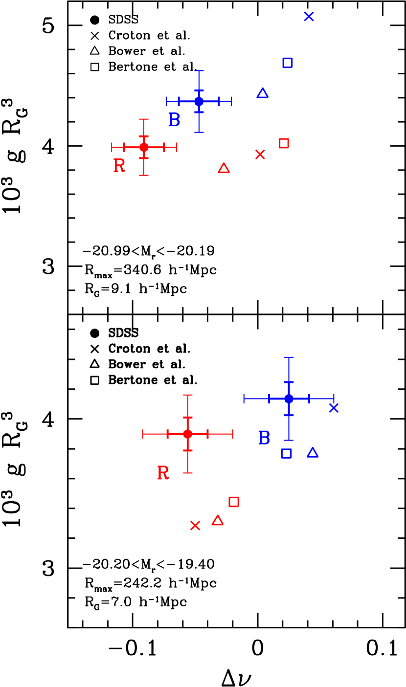
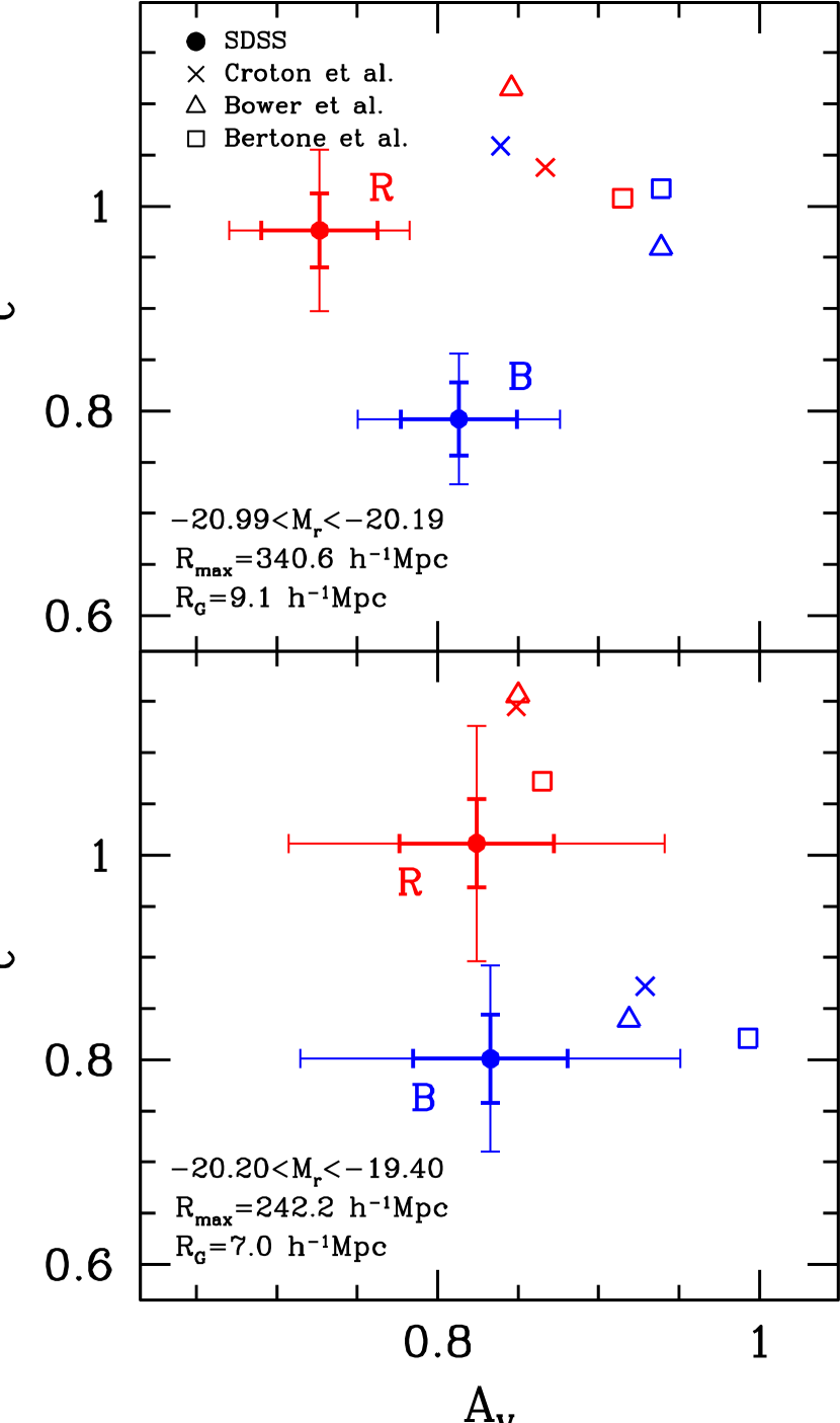
Figure 17 shows the genus-related parameters of the SDSS galaxies (filled circles with error bars) and mock galaxies (other symbols). The upper panels are for the relatively brighter sample of galaxies in L1, and the lower ones are for those in L2. We show two sets of error bars for the observational data points. The shorter ones should be used when difference between blue and red color subsets is a matter of concern, but the longer ones, to which the cosmic variance is included, should be looked at when a model is compared with the observation.

It can be seen in Figure 17 that SAM predictions of the color-dependence of topology are often qualitatively correct but incorrect in magnitude. Failure of the SAM models in reproducing the observed clustering topology of color subsets is more evident for the bright blue galaxies of Croton et al. (2006) in the upper left panel of Figure 17. They have too high genus density and their difference in $g$ with red galaxies is too large. All three models predict relatively too positive $\Delta\nu$ for both red and blue galaxies compared with the combined sample. The right panels of Figure 17 show that $A_{V}$ of both red and blue mock galaxies is again too large in all three SAM model compared with the combined sample. In the case of Bertone et al. and Croton et al., the $A_{V}$ and $A_{C}$ parameters of the brighter sample (upper right panel) are nearly the same for red and blue subsets, which clearly contradicts the observations.

To summarize, the SAM models fail to reproduce the observed clustering topology of galaxies divided according to color. Their problems for the combined sample persist in the color subsets, and new problems are added. In particular, disagreement with the observation is more serious for bright galaxies. There should be more bright blue galaxies in superclusters so that clusters are more connected in the distribution of bright blue galaxies. Both bright blue and red galaxies should be formed less frequently in void regions so that voids can be more connected with one another. The threshold for formation of both red and blue galaxies should be at lower density on average so that the percolation of large-scale structure occurs at lower density.

6. Summary

We use the SDSS DR7 main galaxy catalog supplemented with missing redshifts and with increased spectroscopic completeness to measure the galaxy clustering topology over a range of smoothing scales. The distribution of galaxies observed by the SDSS reveals extremely diverse structures.

A volume-limited sample, BEST defined by $M_{r}<-20.19$ , enables us to measure the genus curve with amplitude of $G=378\pm 18$ at a smoothing scale of $6h^{-1}$ Mpc, with the quoted uncertainty including all systematics and cosmic variance. The amplitude is 5.4 times larger than our previous measurement using the SDSS DR3 sample (Park et al. 2005) and the uncertainty decreases from 10.5% to 4.8% at the same smoothing length of $R_{G}=6h^{-1}$ Mpc. We calculate the galaxy clustering topology over the interval from $R_{G}=6h^{-1}$ Mpc to $10h^{-1}$ Mpc, and find mild scale-dependence for the shift ( $\Delta\nu$ ) and void abundance ( $A_{V}$ ) parameters. The measured genus curve is qualitatively similar to the form predicted for Gaussian primordial fluctuations (Hamilton et al. 1986), but the differences are statistically significant at these scales: a shift of the peak towards negative $\nu$ , and fewer isolated voids and isolated clusters than the Gaussian prediction ( $A_{C}$ and $A_{V}<1$ ). The bias in topology of galaxy clustering with respect to that of matter is measured by assuming that the matter density field is given by our $\Lambda$ CDM N-body simulation. We detect strong topology bias in galaxy clustering, which is also scale-dependent.

We confirm the luminosity dependence of galaxy clustering topology discovered by Park et al. (2005). The distribution of brighter galaxies is more shifted towards “meatball’ topology (lower $\Delta\nu$ ) and shows greater percolation of voids (lower $A_{V}$ ). We find galaxy clustering topology depends also on morphology and color. Even though early (late)-type galaxies show topology similar to that of red (blue) galaxies, morphology-dependence of topology is not identical with color-dependence. In particular, the void abundance parameter $A_{V}$ depends on morphology more strongly than color.

We tested five galaxy formation models, which are used to assign galaxies to the outputs of N-body simulations. Three of these are semi-analytic models, one is an HOD model that assigns galaxies to halos with parameters tuned to match other clustering statistics, and one is a scheme that assigns galaxies to halos and subhalos. None of them reproduces all aspects of the observed topology, though the differences from one model to another are comparable to the discrepancies with the observations. For this reason, and because the initially Gaussian $\Lambda$ CDM model successfully reproduce the observed topology of LRGs at large scales, we attribute the discrepancies to failures of the galaxy formation model rather than non-Gaussian initial conditions. The semi-analytic models can also predict the topology of color subsets, but none of them fully captures the observed topology differences between red and blue galaxies.

In future work, we will investigate models with non-Gaussian initial conditions to see what levels of primordial non-Gaussianity can be ruled out by our measurements. In principle, the high-precision topology measurements presented here and by Gott et al. (2009) can provide valuable constraints on non-standard inflationary models or alternative hypotheses for the origin of primordial fluctuations.

Appendix A details our estimates of systematic biases in the genus curve measurements, demonstrating that the dominant effect is peculiar velocity distortions in redshift space rather than sample geometry or boundary effects. Except where noted otherwise, observational measurements in this paper are corrected for these biases, so they can be compared to theoretical predictions in real space with periodic boundaries. Appendix B investigates error covariances, showing that while the individual points on the genus curve have strongly covariant errors, the statistics $G$ , $\Delta\nu$ , $A_{V}$ , and $A_{C}$ are approximately independent. Appendix C tabulates the full genus curves for our best samples, complementing the statistics recorded in earlier tables.

While future surveys will use luminous galaxies and emission-line galaxies to probe structure in the distant universe, the SDSS DR7 sample is likely to remain the definitive map of large scale structure at low redshift traced by a broad spectrum of galaxy types, for the foreseeable future. The measurements in this paper characterize the topology of this definitive sample, attaining unprecedented statistical precision and providing a valuable test for future models of primordial fluctuations and galaxy formation physics.

We thank Xiaohu Yang for providing us with the HOD data. YYC was supported by a grant from the Kyung Hee University in 2010 (KHU-20100179). CBP acknowledges the support of the National Research Foundation of Korea (NRF) grant funded by the Korea government MEST (No. 2009-0062868). JRG is supported by NSF GRANT AST 04-06713. DHW acknowledges the support of NSF Grant AST-0707985 and an AMIAS membership at the IAS. MSV acknowledges the support of NSF GRANT AST-0507647. SSK was supported by WCU program (R31-1001) and by Basic Science Research Program (2009-0086824), both through the NRF funded by the MEST of Korea. The Millennium Simulation databases used in this paper and the web application providing online access to them were contructed as part of the activities of the German Astrophysical Virtual Observatory. Funding for the SDSS and SDSS-II has been provided by the Alfred P. Sloan Foundation, the Participating Institutions, the National Science Foundation, the U.S. Department of Energy, the National Aeronautics and Space Administration, the Japanese Monbukagakusho, the Max Planck Society, and the Higher Education Funding Council for England. The SDSS Web Site is http://www.sdss.org/. The SDSS is managed by the Astrophysical Research Consortium for the Participating Institutions. The Participating Institutions are the American Museum of Natural History, Astrophysical Institute Potsdam, University of Basel, Cambridge University, Case Western Reserve University, University of Chicago, Drexel University, Fermilab, the Institute for Advanced Study, the Japan Participation Group, Johns Hopkins University, the Joint Institute for Nuclear Astrophysics, the Kavli Institute for Particle Astrophysics and Cosmology, the Korean Scientist Group, the Chinese Academy of Sciences (LAMOST), Los Alamos National Laboratory, the Max-Planck-Institute for Astronomy (MPIA), the Max-Planck-Institute for Astrophysics (MPA), New Mexico State University, Ohio State University, University of Pittsburgh, University of Portsmouth, Princeton University, the United States Naval Observatory, and the University of Washington. This research has made use of the NASA/IPAC Extragalactic Database (NED) which is operated by the Jet Propulsion Laboratory, California Institute of Technology, under contract with the National Aeronautics and Space Administration.

Appendix A Effects of Survey Systematics on the Genus Curve

In this paper we present the observed genus-related statistics corrected for the systematic effects. We aim to obtain the statistics in real space with no boundary and angular selection effects. Such results can be readily compared with theoretical predictions calculated from mock galaxies simulated in a variety of cosmological models without going through a full analysis taking into account the peculiar velocities and the complicated angular and radial survey selection functions of a particular survey. To understand the effects of the systematics on the genus curve step-by-step, we first calculate the genus curve from the number density field of the halos with $M_{h}>7.9\times 10^{11}h^{-1}M_{\odot}$ ( ${\bar{d}}=6.1h^{-1}$ Mpc) in the whole simulation cube (S1 simulation) using periodic boundary conditions. The halos are the ones identified in our $\Lambda$ CDM simulation, which consist of the isolated halos, the central halos, and the satellite subhalos. Each of the halos is assumed to contain one galaxy.

The blue solid line in the top panel of Figure 18 is the corresponding genus curve when $R{{}_{G}}=6h^{-1}$ Mpc.

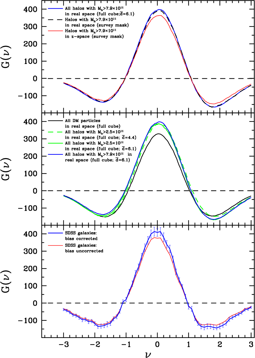
This is the true genus curve we hope to measure with no RSD effects and no survey boundary effects (but with some shot noise effects). We then make 27 mock surveys of these ‘galaxies’ in the simulation cube with radial boundaries and angular selection function identical to SDSS DR7 trimmed as shown in Figure 1. The mock galaxies are located at their real-space positions, and the resulting mock survey samples are free of the RSD effects. The short-dashed line in the top panel of Figure 18 is the genus curve averaged over these 27 samples. It can be seen that the radial boundary and angular selection effects introduce little change in the genus curve in the case of the main part of SDSS DR7 thanks to the large volume-to-surface ratio and high and uniform angular selection function of the sample. A large bias in the genus curve is generated when galaxies are observed in redshift space. The red line in the top panel of Figure 18 is the case when both RSD effects and the effects due to survey boundaries and angular selection function are taken into account in the 27 mock SDSS DR7 surveys. The difference between red line and dashed line is due to the RSD effects. The amplitude of the genus curve is decreased mostly due to the smoothing of structure by small-scale peculiar velocities of galaxies, but its shape does not change much. The genus curve near the median-volume threshold $(\nu=0)$ is slightly pushed to the negative threshold direction, thus making $\Delta\nu$ decrease. Both the number of clusters and voids are decreased. The number of high density regions is decreased more because massive clusters of galaxies are strongly clustered with one another and two clusters often appear connected along the line-of-sight in redshift space. On the other hand, a void can be affected when strong fingers-of-God protrude into the void from surrounding clusters in redshift space. The number of voids is decreased only a little between the blue and red lines in the top panel of Figure 18 because it is difficult for voids identified on $R{{}_{G}}=6h^{-1}$ Mpc scale to be erased by this process. But the number of voids relative to those expected from the best-fitting Gaussian curve ( $A_{V}$ ) is rather increased.

It is also interesting to know how the genus curve depends on the type of the density tracer. A comprehensive study on this issue has been made by Park, Kim & Gott (2005), who used a set of N-body simulations of $\Lambda$ CDM and the Standard Cold Dark Matter Universe to examine the dependence of the genus curve on gravitational evolution, biasing, RSD, smoothing scale, and cosmology. In the middle panel of Figure 18 we show how the genus curve changes at $R{{}_{G}}=6h^{-1}$ Mpc scale as the density tracer changes from dark matter particles to dark halos with different mass limits. The genus curve for the halos with $M_{h}>7.9\times 10^{11}h^{-1}M_{\odot}$ ( $\bar{d}=6.1h^{-1}$ Mpc) is plotted by a blue solid line again. The green solid line is the genus curve for the less massive halos with mass $M_{h}>2.5\times 10^{11}h^{-1}M_{\odot}$ that are sparsely sampled to match the mean galaxy separation to $6.1h^{-1}$ Mpc. The green dashed line is for the full less massive halo data with $\bar{d}=4.4h^{-1}$ Mpc. The figure demonstrates the dark matter density field (black solid line) and the halo number density fields (blue solid line) have very different topology at $6h^{-1}$ Mpc Gaussian smoothing scale. The $\Delta\nu$ parameter is positive for both matter particles and halo. The $A_{V}$ and $A_{C}$ parameters for matter are close to 1 and much larger than those of halos. For the $A_{V}$ parameter, the difference is much larger. The strong bias in the observed clustering topology of the SDSS galaxies with respect to that of matter is shown in Figure 8. On the other hand, the relatively more massive halos with $M_{h}>7.9\times 10^{11}h^{-1}M_{\odot}$ describe fewer superclusters or fewer voids at fixed volume fractions (smaller $A_{V}$ and $A_{C}$ ) when compared with that of halos with $M_{h}>2.5\times 10^{11}h^{-1}M_{\odot}$ .

Appendix B Covariance matrix of the Genus-related statistics

To understand how the measurements of the genus at different levels are correlated with one another, in Figure 19 we show the covariance matrix

c_{ij}={{<\delta G_{i}\delta G_{j}>}\over{\sigma_{i}\sigma_{j}}}

(B1)

where $\delta G_{i}=G(\nu_{i})-\bar{G}(\nu_{i})$ is the difference of the genus from the mean at a threshold $\nu_{i}$ , and $\sigma_{i}$ is the standard deviation of the genus at $\nu_{i}$ . Estimation is made using two $\Lambda$ CDM simulations, S1 and S2. (See Table 2 for simulation parameters. Detailed explanation of these simulations is given in section 4.2.)

The bottom panel of Figure 19 shows the covariance measured from the halos with $\bar{d}=6.1{h^{-1}\,{\rm Mpc}}$ . The whole simulation cube of the S2 simulation with size of 1433.6 $h^{-1}$ Mpc is divided into 64 subcubes of size $358.4{h^{-1}\,{\rm Mpc}}$ , and the 64 genus curves from these subcubes are used to calculate the matrix. The filled and open circles represent positive and negative covariances, respectively. The covariance along the diagonal line is one by definition, and the radius of circles are proportional to the covariance. The covariance plot in the upper panel is obtained from the matter particles with $\bar{d}=0.5{h^{-1}\,{\rm Mpc}}$ of the S1 simulation divided into 512 subcubes of size $128.0{h^{-1}\,{\rm Mpc}}$ . In both plots a smoothing length of $R_{G}=6.0{h^{-1}\,{\rm Mpc}}$ is used.

The covariance seems to be smallest for threshold levels $\nu=0$ , and $\pm\sqrt{3}$ , where the extrema of the genus curve are located (see Gott et al. 1990 for a similar finding for $\nu=0$ level). There is a positive covariance strip along the diagonal with a width of about $\sqrt{3}/2$ with the width of positive and negative correlation ranges slightly depending on $\nu$ . There are also two negative covariance strips shifted from the diagonal by $\pm\sqrt{3}$ , two positive ones with shifts of $\pm 2\sqrt{3}$ , and so on. The magnitude of the covariance decreases rather slowly from the diagonal.

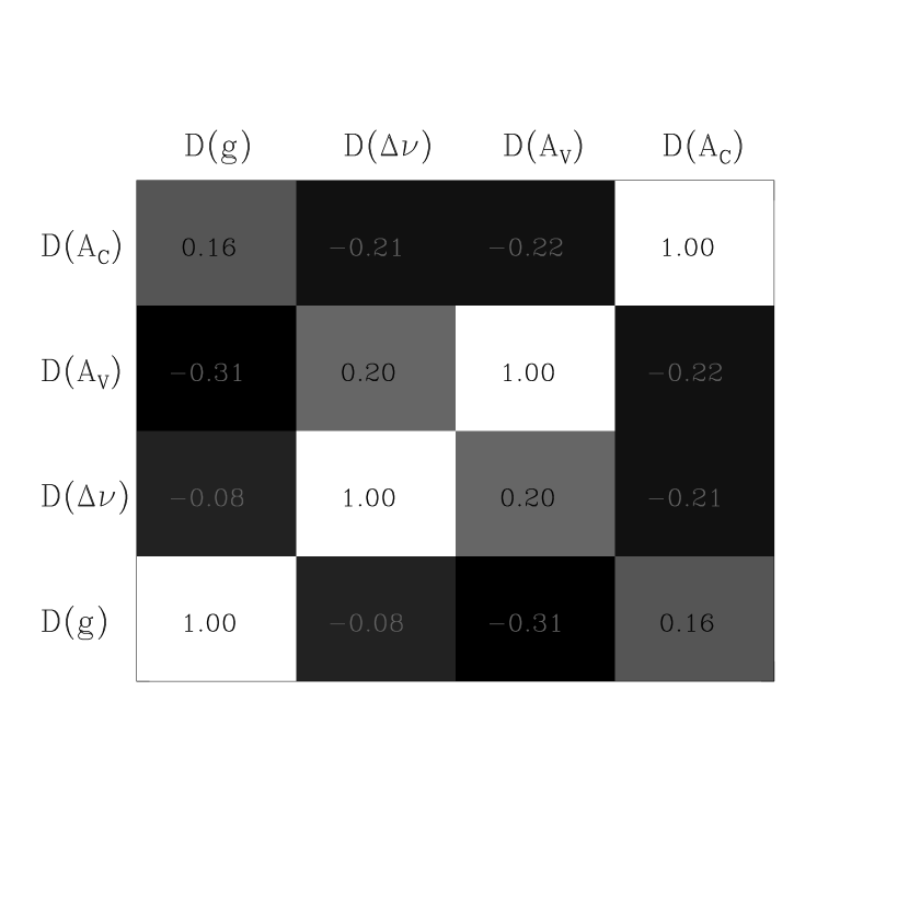
To understand how the genus-related statistics employed in this paper are correlated with one another, we calculate the covariance matrix

d_{ij}={{<\Delta u_{i}\Delta u_{j}>}\over{s_{i}s_{j}}},

(B2)

where $u_{i}$ is the $i$ -th one of the four genus-related statistics, $\Delta u_{i}=u_{i}-{\bar{u}_{i}}$ , and ${\bar{u}_{i}}$ is the mean of the $i$ -th statistic calculated from 512 genus curves of the dark matter particles in the 512 subcubes of size 128 $h^{-1}$ Mpc taken from the S1 simulation. The smoothing length used is $R_{G}=3h^{-1}$ Mpc. The average in Equation (B2) is taken over 512 subcubes, and $s_{i}$ is the standard deviation of the $i$ -th statistic from its mean. The matrix is symmetric, and its diagonal elements are one by definition. Figure 19 shows that the genus-related statistics are roughly independent of one another, with the magnitude of the covariance ranging from 0.08 to 0.31. Thus, it is roughly acceptable to test a model using a simple $\chi^{2}$ -test with these four statistics and the quoted observational errors, ignoring covariance, a conclusion further supported by the mock catalog tests shown in Figure 16.

Appendix C Table of Genus Curves

In this section, we give the tables of the genus curves for the convenience of readers who wish to use galaxy clustering topology to test their galaxy formation or cosmological models. In Table 9 the genus is given as a function of volume-fraction threshold level for the observational morphology and color subsamples. The genus curves for the SDSS galaxies in the BEST sample and the five sets of mock galaxies measured in Section $5.2$ are given in Table 10. The genus values of the SDSS galaxies are corrected for the systematic biases, and the uncorrected values are in parentheses. These two curves are plotted in the bottom panel of Figure 18. Electronic forms of these tables are available from the authors on request. Models can also be tested against the genus curve statistics reported in earlier tables.

Table 9The Genus values at a given threshold level of the Morphology and Color Samples in Figure 12 and 17

$\nu$	$-20.19<M{{}_{r}}<-20.99$		$-19.40<M_{r}<-20.40$		$-20.19<M_{r}<-20.99$		$-19.40<M_{r}<-20.40$
	( $R_{G}=9.1{h^{-1}\,{\rm Mpc}}$ )		( $R_{G}=7.9{h^{-1}\,{\rm Mpc}}$ )		( $R_{G}=9.1{h^{-1}\,{\rm Mpc}}$ )		( $R_{G}=7.0{h^{-1}\,{\rm Mpc}}$ )
	Early	Late	Early	Late	Red	Blue	Red	Blue
$-3.0$	$-14.8$	$-14.0$	$-8.8$	$-7.0$	$-13.7$	$-12.6$	$-9.7$	$-7.1$
$-2.9$	$-17.8$	$-17.1$	$-9.4$	$-7.2$	$-20.5$	$-17.3$	$-16.5$	$-10.0$
$-2.8$	$-17.4$	$-19.6$	$-12.2$	$-14.3$	$-24.2$	$-21.8$	$-18.8$	$-12.4$
$-2.7$	$-21.0$	$-24.3$	$-14.8$	$-15.5$	$-23.9$	$-28.6$	$-15.7$	$-13.7$
$-2.6$	$-22.8$	$-28.5$	$-14.3$	$-17.8$	$-28.1$	$-34.8$	$-18.4$	$-18.4$
$-2.5$	$-30.4$	$-32.8$	$-14.6$	$-19.8$	$-30.2$	$-35.8$	$-15.8$	$-20.2$
$-2.4$	$-29.2$	$-36.6$	$-18.7$	$-20.9$	$-32.5$	$-38.9$	$-22.6$	$-23.6$
$-2.3$	$-35.4$	$-43.0$	$-21.8$	$-21.9$	$-44.1$	$-39.6$	$-25.1$	$-26.4$
$-2.2$	$-38.8$	$-46.4$	$-21.0$	$-21.9$	$-43.1$	$-42.8$	$-28.4$	$-26.2$
$-2.1$	$-42.7$	$-47.2$	$-19.0$	$-26.3$	$-40.3$	$-42.4$	$-32.7$	$-35.6$
$-2.0$	$-36.7$	$-47.4$	$-22.6$	$-25.9$	$-38.7$	$-43.2$	$-37.4$	$-35.8$
$-1.9$	$-40.1$	$-40.1$	$-18.8$	$-25.0$	$-34.4$	$-48.3$	$-38.4$	$-38.0$
$-1.8$	$-39.2$	$-43.1$	$-26.1$	$-32.4$	$-37.5$	$-50.4$	$-34.8$	$-42.1$
$-1.7$	$-37.1$	$-54.6$	$-25.1$	$-29.1$	$-40.5$	$-45.7$	$-41.4$	$-44.5$
$-1.6$	$-39.4$	$-57.9$	$-23.5$	$-20.2$	$-37.7$	$-40.9$	$-35.9$	$-31.1$
$-1.5$	$-26.5$	$-48.2$	$-24.7$	$-21.5$	$-37.4$	$-39.7$	$-29.1$	$-27.1$
$-1.4$	$-23.9$	$-44.0$	$-24.8$	$-23.1$	$-36.3$	$-36.9$	$-23.5$	$-29.3$
$-1.3$	$-20.8$	$-34.9$	$-20.4$	$-24.6$	$-22.6$	$-43.1$	$-14.0$	$-22.9$
$-1.2$	$-16.5$	$-34.4$	$-4.4$	$-11.7$	$-11.0$	$-35.6$	$-13.2$	$-19.4$
$-1.1$	$3.2$	$-27.7$	$4.3$	$-4.1$	$4.7$	$-21.2$	$-19.7$	$-10.4$
$-1.0$	$24.3$	$-5.2$	$5.7$	$-1.5$	$32.1$	$2.1$	$1.5$	$-0.3$
$-0.9$	$55.0$	$17.9$	$25.9$	$1.0$	$28.4$	$26.3$	$31.8$	$18.6$
$-0.8$	$65.0$	$49.7$	$28.3$	$16.5$	$46.7$	$31.6$	$43.1$	$21.1$
$-0.7$	$79.5$	$57.3$	$41.2$	$30.4$	$78.7$	$45.9$	$43.6$	$32.5$
$-0.6$	$100.7$	$83.1$	$49.6$	$30.6$	$91.1$	$69.9$	$53.5$	$47.3$
$-0.5$	$112.1$	$92.9$	$37.8$	$37.3$	$105.7$	$78.6$	$77.4$	$51.5$
$-0.4$	$123.0$	$82.0$	$48.3$	$36.8$	$124.3$	$108.9$	$79.9$	$68.1$
$-0.3$	$123.6$	$121.5$	$62.0$	$41.9$	$124.0$	$137.4$	$85.5$	$86.4$
$-0.2$	$113.3$	$151.4$	$68.9$	$52.8$	$124.7$	$146.1$	$90.4$	$100.5$
$-0.1$	$118.9$	$173.3$	$63.9$	$65.5$	$111.2$	$153.0$	$94.8$	$98.5$
$0.0$	$134.5$	$161.1$	$68.6$	$65.2$	$127.0$	$150.1$	$97.6$	$102.8$
$0.1$	$119.0$	$157.0$	$59.2$	$68.9$	$111.5$	$143.5$	$95.5$	$110.6$
$0.2$	$111.7$	$118.4$	$58.1$	$66.8$	$114.3$	$128.1$	$74.5$	$96.6$
$0.3$	$85.5$	$112.1$	$54.6$	$68.9$	$81.4$	$100.9$	$69.6$	$83.9$
$0.4$	$77.7$	$96.4$	$51.0$	$65.2$	$81.9$	$104.2$	$78.4$	$84.9$
$0.5$	$73.8$	$84.3$	$40.1$	$56.7$	$72.5$	$85.0$	$62.3$	$76.9$
$0.6$	$52.9$	$60.8$	$33.7$	$35.4$	$60.1$	$55.0$	$48.8$	$63.1$
$0.7$	$44.2$	$32.8$	$25.7$	$29.3$	$49.1$	$44.2$	$33.4$	$34.9$
$0.8$	$22.1$	$7.5$	$9.5$	$7.9$	$28.1$	$15.5$	$21.1$	$28.9$
$0.9$	$6.9$	$-18.7$	$4.0$	$-6.8$	$1.9$	$-11.9$	$12.1$	$14.5$
$1.0$	$-12.7$	$-32.6$	$0.1$	$-10.7$	$-20.6$	$-20.2$	$-4.2$	$-1.0$
$1.1$	$-32.1$	$-35.0$	$-14.2$	$-10.0$	$-35.5$	$-22.1$	$126.7$	$90.8$
$1.2$	$-44.2$	$-48.6$	$-31.4$	$-15.4$	$-37.6$	$-30.4$	$-36.4$	$-22.8$
$1.3$	$-57.6$	$-36.1$	$-37.1$	$-26.5$	$-49.3$	$-26.8$	$-40.0$	$-20.5$
$1.4$	$-50.6$	$-30.9$	$-31.1$	$-25.1$	$-45.5$	$-37.9$	$-45.4$	$-31.9$
$1.5$	$-47.4$	$-34.5$	$-30.3$	$-23.8$	$-53.5$	$-45.7$	$-44.0$	$-30.5$
$1.6$	$-46.0$	$-37.7$	$-33.5$	$-25.1$	$-70.6$	$-53.9$	$-40.3$	$-35.7$
$1.7$	$-50.7$	$-44.9$	$-30.2$	$-26.7$	$-56.6$	$-43.3$	$-38.1$	$-38.5$
$1.8$	$-50.5$	$-46.1$	$-23.6$	$-23.5$	$-45.1$	$-42.7$	$-29.4$	$-39.7$
$1.9$	$-40.5$	$-52.7$	$-25.9$	$-20.2$	$-38.0$	$-43.5$	$-33.5$	$-27.3$
$2.0$	$-35.9$	$-46.2$	$-25.7$	$-16.4$	$-36.6$	$-48.6$	$-32.0$	$-29.5$
$2.1$	$-37.0$	$-42.0$	$-20.1$	$-16.1$	$-42.7$	$-42.9$	$-31.3$	$-30.4$
$2.2$	$-38.1$	$-32.5$	$-19.7$	$-14.9$	$-34.3$	$-40.0$	$-32.5$	$-31.3$
$2.3$	$-33.6$	$-35.8$	$-14.9$	$-14.3$	$-33.9$	$-35.6$	$-25.6$	$-21.5$
$2.4$	$-28.7$	$-30.7$	$-15.2$	$-12.1$	$-29.7$	$-29.2$	$-20.0$	$-17.6$
$2.5$	$-24.8$	$-26.1$	$-11.5$	$-11.7$	$-25.9$	$-26.4$	$-16.0$	$-15.7$
$2.6$	$-19.4$	$-22.8$	$-13.6$	$-10.0$	$-18.2$	$-24.6$	$-16.9$	$-15.6$
$2.7$	$-17.5$	$-20.3$	$-11.7$	$-9.0$	$-14.1$	$-21.7$	$-15.7$	$-15.2$
$2.8$	$-12.0$	$-18.4$	$-9.8$	$-6.9$	$-13.3$	$-16.6$	$-11.8$	$-13.1$
$2.9$	$-8.6$	$-11.9$	$-8.8$	$-4.3$	$-11.8$	$-11.5$	$-7.4$	$-9.8$
$3.0$	$-7.3$	$-11.0$	$-5.6$	$-4.6$	$-8.2$	$-10.7$	$-5.9$	$-3.1$

Note. All the values are systematic bias-corrected.

Table 10The Genus at a given threshold level of the Samples in Figure 15

$\nu$	$G(\nu)_{\rm SDSS}$	$G(\nu)_{\mathrm{HGC}}$	$G(\nu)_{\mathrm{Bertone}}$	$G(\nu)_{\mathrm{HOD}}$	$G(\nu)_{\mathrm{Croton}}$	$G(\nu)_{\mathrm{Bower}}$
$-3.0$	$-37.2(-33.6)\pm 6.6$	$-27.0$	$-31.0$	$-30.2$	$-30.4$	$-36.8$
$-2.9$	$-43.1(-37.0)\pm 7.3$	$-35.4$	$-38.0$	$-37.0$	$-35.5$	$-43.0$
$-2.8$	$-53.3(-45.5)\pm 7.9$	$-43.1$	$-45.4$	$-43.8$	$-46.9$	$-51.0$
$-2.7$	$-67.9(-62.5)\pm 8.2$	$-50.9$	$-54.3$	$-52.8$	$-55.1$	$-60.2$
$-2.6$	$-72.2(-65.8)\pm 8.8$	$-60.0$	$-62.3$	$-61.9$	$-65.6$	$-70.1$
$-2.5$	$-83.2(-76.1)\pm 10.8$	$-70.8$	$-70.5$	$-72.2$	$-77.9$	$-80.2$
$-2.4$	$-96.5(-88.8)\pm 10.8$	$-82.6$	$-84.7$	$-82.9$	$-90.9$	$-90.9$
$-2.3$	$-93.9(-88.1)\pm 10.1$	$-93.4$	$-97.1$	$-95.8$	$-98.9$	$-105.7$
$-2.2$	$-107.0(-99.5)\pm 11.3$	$-105.4$	$-116.2$	$-109.8$	$-109.6$	$-118.7$
$-2.1$	$-104.5(-98.2)\pm 9.8$	$-116.1$	$-129.2$	$-125.7$	$-125.9$	$-133.5$
$-2.0$	$-118.6(-112.7)\pm 10.8$	$-124.1$	$-145.2$	$-141.1$	$-136.6$	$-146.5$
$-1.9$	$-135.0(-124.0)\pm 10.5$	$-131.6$	$-149.5$	$-149.5$	$-149.7$	$-157.8$
$-1.8$	$-132.2(-122.1)\pm 12.1$	$-136.0$	$-152.0$	$-153.9$	$-151.0$	$-168.1$
$-1.7$	$-130.1(-123.7)\pm 11.6$	$-136.6$	$-148.1$	$-151.8$	$-148.1$	$-163.9$
$-1.6$	$-121.6(-115.2)\pm 15.5$	$-131.0$	$-145.4$	$-145.0$	$-136.4$	$-161.7$
$-1.5$	$-116.3(-108.1)\pm 12.5$	$-120.0$	$-134.3$	$-132.1$	$-131.0$	$-153.4$
$-1.4$	$-90.8(-84.3)\pm 11.7$	$-104.4$	$-115.8$	$-112.1$	$-110.0$	$-129.4$
$-1.3$	$-78.9(-72.2)\pm 11.9$	$-83.3$	$-89.7$	$-96.5$	$-84.3$	$-104.7$
$-1.2$	$-47.7(-43.1)\pm 10.3$	$-55.5$	$-60.0$	$-69.3$	$-52.2$	$-74.0$
$-1.1$	$8.0(7.6)\pm 10.6$	$-24.5$	$-31.4$	$-31.0$	$-17.2$	$-37.6$
$-1.0$	$19.7(19.3)\pm 12.1$	$14.8$	$6.1$	$10.0$	$13.3$	$6.9$
$-0.9$	$66.7(57.2)\pm 12.6$	$59.4$	$60.0$	$58.6$	$63.3$	$48.7$
$-0.8$	$112.0(101.1)\pm 15.7$	$102.9$	$112.1$	$105.1$	$109.2$	$98.5$
$-0.7$	$169.4(153.2)\pm 18.3$	$152.2$	$147.1$	$156.7$	$155.3$	$159.8$
$-0.6$	$208.7(192.5)\pm 17.1$	$201.1$	$200.4$	$205.1$	$204.9$	$218.3$
$-0.5$	$267.3(247.8)\pm 19.3$	$250.7$	$247.7$	$254.3$	$247.7$	$260.9$
$-0.4$	$320.3(296.7)\pm 21.9$	$296.0$	$295.8$	$294.4$	$295.6$	$293.0$
$-0.3$	$362.4(334.0)\pm 22.0$	$335.2$	$338.6$	$340.9$	$329.8$	$339.5$
$-0.2$	$399.1(366.7)\pm 23.3$	$368.5$	$373.8$	$369.3$	$350.2$	$369.1$
$-0.1$	$413.3(379.0)\pm 25.9$	$385.9$	$389.7$	$383.1$	$369.5$	$384.9$
$0.0$	$408.9(374.6)\pm 23.0$	$395.0$	$407.4$	$403.0$	$388.0$	$399.5$
$0.1$	$413.4(376.7)\pm 23.1$	$398.3$	$409.6$	$402.6$	$372.2$	$405.5$
$0.2$	$379.9(344.0)\pm 25.8$	$387.7$	$398.3$	$385.3$	$354.9$	$394.8$
$0.3$	$339.6(308.6)\pm 21.1$	$362.0$	$368.7$	$361.9$	$329.8$	$373.0$
$0.4$	$312.7(279.8)\pm 21.5$	$329.4$	$331.6$	$326.5$	$296.9$	$332.7$
$0.5$	$253.7(226.8)\pm 18.4$	$289.4$	$286.8$	$295.2$	$254.7$	$293.4$
$0.6$	$180.8(161.2)\pm 16.3$	$245.1$	$239.0$	$250.0$	$206.3$	$245.0$
$0.7$	$133.5(120.6)\pm 12.6$	$191.8$	$193.4$	$186.2$	$159.8$	$194.0$
$0.8$	$94.3(85.6)\pm 12.8$	$140.3$	$139.9$	$132.3$	$110.2$	$135.8$
$0.9$	$38.5(33.0)\pm 13.4$	$89.0$	$90.1$	$74.6$	$57.4$	$85.5$
$1.0$	$-19.7(-15.6)\pm 14.8$	$35.8$	$37.4$	$32.5$	$3.0$	$19.9$
$1.1$	$-32.6(-33.8)\pm 14.4$	$-11.9$	$-19.9$	$-26.5$	$-39.5$	$-29.8$
$1.2$	$-87.8(-80.7)\pm 13.6$	$-53.9$	$-61.9$	$-68.7$	$-73.4$	$-65.4$
$1.3$	$-117.6(-108.8)\pm 11.6$	$-87.4$	$-93.8$	$-103.0$	$-107.6$	$-101.6$
$1.4$	$-135.0(-124.8)\pm 13.3$	$-113.9$	$-121.6$	$-127.5$	$-129.6$	$-121.1$
$1.5$	$-139.7(-125.3)\pm 14.3$	$-137.4$	$-141.7$	$-146.0$	$-148.9$	$-143.2$
$1.6$	$-134.0(-122.1)\pm 14.3$	$-152.9$	$-153.7$	$-163.7$	$-160.9$	$-159.4$
$1.7$	$-135.6(-121.3)\pm 12.4$	$-162.8$	$-156.5$	$-172.8$	$-170.1$	$-167.4$
$1.8$	$-140.0(-124.8)\pm 13.6$	$-165.2$	$-158.8$	$-168.3$	$-169.9$	$-170.7$
$1.9$	$-143.5(-127.3)\pm 11.1$	$-161.0$	$-158.6$	$-169.3$	$-168.3$	$-166.4$
$2.0$	$-135.7(-119.5)\pm 12.5$	$-156.8$	$-155.7$	$-160.2$	$-158.2$	$-158.0$
$2.1$	$-127.6(-111.7)\pm 11.8$	$-146.5$	$-147.7$	$-149.1$	$-149.7$	$-144.8$
$2.2$	$-116.8(-100.0)\pm 11.3$	$-134.4$	$-133.7$	$-141.9$	$-132.7$	$-137.0$
$2.3$	$-93.0(-81.1)\pm 11.3$	$-121.5$	$-116.0$	$-129.4$	$-118.3$	$-122.8$
$2.4$	$-84.4(-71.3)\pm 8.6$	$-110.9$	$-100.8$	$-114.4$	$-104.1$	$-108.8$
$2.5$	$-73.7(-63.6)\pm 7.2$	$-97.4$	$-91.1$	$-96.9$	$-91.7$	$-91.3$
$2.6$	$-64.4(-54.7)\pm 8.6$	$-83.6$	$-77.1$	$-81.0$	$-77.3$	$-79.8$
$2.7$	$-54.6(-47.2)\pm 8.4$	$-71.2$	$-62.5$	$-68.5$	$-63.7$	$-66.6$
$2.8$	$-38.1(-31.6)\pm 8.1$	$-61.3$	$-51.0$	$-55.9$	$-52.4$	$-54.3$
$2.9$	$-34.5(-29.0)\pm 7.1$	$-49.2$	$-43.4$	$-44.0$	$-44.2$	$-44.8$
$3.0$	$-23.4(-19.3)\pm 6.0$	$-39.4$	$-37.4$	$-37.0$	$-34.9$	$-37.2$

Note. Genus values at a given threshold level of the SDSS galaxies in the BEST sample and five sets of the mock galaxies. The density fields were smoothed smoothing scale $R_{G}$ is $6.0{h^{-1}\,{\rm Mpc}}$ . The genus values of the SDSS galaxies are systematic bias-corrected and the observed values are given in parentheses.

References

Abazajian et al. (200) Abazajian, K. N., et al. 2009, ApJS, 182, 543
Bardeen et al. (1986) Bardeen, J. M., Bond, J. R., Kaiser, N., & Szalay, A. S. 1986, ApJ, 304, 15
Benson et al. (2002) Benson, A. J., Lacey, C. G., Baugh, C. M., Cole, S., Frenk, C. S. 2002, MNRAS, 333, 156
Berlind & Weinberg (2002) Berlind, A. A., & Weinberg, D. H. 2002, ApJ, 575, 587
Berlind et al. (2003) Berlind, A. A., et al. 2003, ApJ, 593, 587
Bertone et al. (2005) Bertone, S., Stoehr, F., & White, S. D. M. 2005, MNRAS, 359, 1201
Bertone et al. (2007) Bertone, S., De Lucia, G., & Thomas, P. A. 2007, MNRAS, 379, 1143
Blanton et al. (2003) Blanton, M. R., Lin, H., Lupton, R. H., Maley, F. M., Young, N., Zehavi, I., & Loveday, J. 2003, AJ, 125, 2276
Blanton et al. (2005) Blanton, M. R., et al. 2005, ApJ, 129, 2562
Bower et al. (2006) Bower, R. G., Benson, A. J., Malbon, R., Helly, J. C., Frenk, C. S., Baugh, C. M., Cole, S., & Lacey, C. G. 2006, MNRAS, 370, 645
Cattaneo et al. (2006) Cattaneo, A., Dekel, A., Devriendt, J., Guiderdoni, B., Blaizot, J. 2006, MNRAS, 370, 1651
Canavezes et al. (1998) Canavezes A. et al., 1998, MNRAS, 297, 777
Colless et al. (2001) Colless, M., et al. 2001, MNRAS, 328, 1039
Cole et al. (2000) Cole, S., Lacey, C. G., Baugh, C. M., Frenk, C. S. 2000, MNRAS, 319, 168
Choi et al. (2010) Choi, Y.-Y., Han, D.-H., & Kim, S. S. 2010, in preparation
Croton et al. (2006) Croton, D. J., et al. 2006, MNRAS, 365, 11
de Vaucouleurs et al. (1991) de Vaucouleurs, G. et al. 1991, Third Reference Catalogue of Bright Galaxies, Volume 1-3, XII (Springer-Verlag)
de Lucia & Blaizot (2007) de Lucia, G., & Blaizot, J. 2007, MNRAS, 375, 2
Doroshkevich, G. (1970) Doroshkevich, G. 1970, Astrophysika, 6, 320
Falco et al. (1999) Falco, E. E., et al. 1999, PASP, 111, 438
Geller & Huchra (1989) Geller, M. J., & Huchra, J. P. 1989, Science, 246, 897
Gott et al. (1986) Gott, J. R., Melott, A. L. & Dickinson, M. 1986, ApJ, 306, 341
Gott et al. (1987) Gott, J. R., Weinberg, D. H., & Melott, A. L. 1987, ApJ, 319, 1
Gott et al. (1996) Gott, J. R., Cen, R., & Ostriker, J. P. 1996, ApJ, 465, 499
Gott et al. (2005) Gott, J. R., et al., 2005, ApJ, 624, 463
Gott et al. (2008) Gott, J. R., et al., 2008, ApJ, 675, 16
Gott et al. (2009) Gott, J. R., Choi, Y.-Y., & Park, C. 2009, ApJ, 695, L45
Hamilton et al. (1986) Hamilton, A. J. S., Gott, J. R., & Weinberg, D. W. 1986, ApJ, 309, 1
Hikage et al. (2002) Hikage C. et al., 2002, PASJ, 54, 707
Hikage et al. (2003) Hikage C. et al., 2003, PASJ, 55, 911
Hikage et al. (2005) Hikage, C., Matsubara, T., Park, M. G., Suto, Y., & Weinberg, D. H. 2005, ApJ, 633, 11
Hoyle et al. (2002) Hoyle, F., et al. 2002, ApJ, 580, 663
Hoyle, Vogeley, & Gott (2002) Hoyle F., Vogeley M. S., Gott J. R. 2002, ApJ, 570, 44
James, Lewis, & Colless (2007) James J. B., Lewis G. F., Colless M., 2007, MNRAS, 375, 128
James et al. (2007) James J. B., Colless M., Lewis G. F., & Peacock, J. A., 2007, MNRAS, 375, 128
Kim & Park (2006) Kim, J., & Park, C. 2006, ApJ, 639, 600
Kim et al. (2009) Kim, J., Park, C., Gott, J. R., & Dubinski, J. 2009, ApJ, 701, 1547
Kang et al. (2002) Kang, X., Jing, Y. P., Mo, H. H., & Borner, G. 2002, MNRAS, 336, 892
Matsubara, T. (1994) Matsubara, T. 1994, ApJ, 434, L43
Matsubara, T. (1996) Matsubara, T. 1996, ApJ, 457, 13
Matsubara & Suto (1996) Matsubara T., & Suto Y. 1996, ApJ, 460, 51
Monaco et al. (2007) Monaco, P., Fontanot, F., Taffoni, G. 2007, MNRAS, 375, 1189
Moore et al. (1992) Moore, B., Frenk, C. S., Weinberg, D. H., Saunders, W., Lawrence, A., Ellis, R. S., Kaiser, N., Efstathiou, G., & Rowan-Robinson, M. 1992, MNRAS, 256, 477
Park et al. (2005b) Park, C., Choi, Y.-Y., Vogeley, M. S., Gott, J. R., Kim, J., Hikage, C., Matsubara, T., Park, M. G., Suto, Y., Weinberg, D. H., & the SDSS Collaboration 2005 $b$ , ApJ, 633, 11
Park et al. (2001) Park, C., Gott, J. R., Choi Y. J., 2001, ApJ, 553, 33
Park & Gott (1991) Park, C., & Gott, J. R. 1991, ApJ, 378, 457
Park et al. (1992) Park, C., Gott, J. R., Melott, A. L., & Karachentsev, I. D. 1992, ApJ, 387, 1
Park, Gott, & da Costa (1992) Park, C., Gott, J. R., da Costa L. N., 1992, ApJ, 392, L51
Park, Kim, & Gott (2005) Park, C., Kim, J., & Gott, J. R. 2005, ApJ, 633, 1
Park & Hwang (2009) Park, C., & Hwang, H. S. 2009, ApJ, 699, 1595
Park, et al. (1994) Park, C., Vogeley, M. S., Geller, J., & Huchra, J. P. 1994, ApJ, 431,569
Rhoads, Gott, & Postman (1994) Rhoads J. E., Gott J. R ., Postman M., 1994, ApJ, 421, 1
Protogeros & Weinberg (1997) Protogeros, Z. A. M., & Weinberg, D. H. 1997, ApJ, 489, 457
Saunders et al. (2000) Saunders, W. et al. 2000, MNRAS, 317, 55
Scoccimarro et al. (2001) Scoccimarro, R., Sheth, R. K., Hui, L., & Jain, B. 2001, ApJ, 546, 20
Somerville et al. (2008) Somerville, R. S., Hopkins, P. F., Cox, T. J., Robertson, B. E., Hernquist, L. 2008, MNRAS, 391, 481
Seljak, U. (2000) Seljak, U. 2000, MNRAS, 318, 203
Stoughton et al. (2002) Stoughton, C., et al. 2002, AJ, 123, 485
Strauss et al. (2002) Strauss, M. A., et al. 2002, AJ, 124, 1810
Sperget et al. (2007) Spergel, D. N., et al. 2007, ApJS, 170, 377
Vogeley et al. (1994) Vogeley, M. S., Park, C., Geller, M. J., Huchra, J. P., & Gott, J. R. 1994, ApJ, 420, 525
Weinberg & Cole (1992) Weinberg, D. H., & Cole, S. 1992, MNRAS, 259, 652
Yang et al. (2007) Yang, X., Mo, H. J., van den Bosch, F. C., Pasquali, A., Li, C., & Barden, M. 2007, ApJ, 671, 153
York et al. (2000) York, D., et al. 2000, AJ, 120, 1579
van den Bosch et al. (2007) van den Bosch, F. C., et al. 2007, MNRAS, 376, 841
Zheng, Coil, & Zehavi (2007) Zheng, Z., Coil, A. L., & Zehavi, I. 2007, ApJ, 667, 760