Time–dependent density functional theory for quantum transport

Abstract

Based on our earlier works [Phys. Rev. B 75, 195127 (2007) & J. Chem. Phys. 128, 234703 (2008)], we propose a formally exact and numerically convenient approach to simulate time–dependent quantum transport from first–principles. The proposed approach combines time–dependent density functional theory with quantum dissipation theory, and results in a useful tool for studying transient dynamics of electronic systems. Within the proposed exact theoretical framework, we construct a number of practical schemes for simulating realistic systems such as nanoscopic electronic devices. Computational cost of each scheme is analyzed, with the expected level of accuracy discussed. As a demonstration, a simulation based on the adiabatic wide–band limit approximation scheme is carried out to characterize the transient current response of a carbon nanotube based electronic device under time–dependent external voltages.

I Introduction

The combined density functional theory (DFT) and nonequilibrium Green’s function (NEGF) approach has been widely employed to simulate steady state quantum electron transport through molecular junctions and other nanoscopic structures. In practice, DFT introduces an effective single–electron reference system, on which NEGF analysis for steady current and electron occupation can be worked out. However, in principle it remains obscure how the conventional DFT for ground/equilibrium state of isolated systems can provide a rigorous framework for quantum transport, as electron transport is intrinsically a dynamic process.

Time–dependent density functional theory (TDDFT)gross has been developed to study quantum transport phenomena.stef ; kurt ; zheng1 ; zheng2 ; zheng3 ; yan1 ; Jin08234703 ; burke ; chen1 As a formally rigorous and numerically tractable approach, TDDFT promises real–time simulations on ultrafast electron transport through realistic electronic devices or structures. In early attempts, finite source–device–drain systems were treated by the conventional TDDFT for isolated systems.aiichiro ; voor ; ventra Since the source and drain were treated as finite, the results were not directly transferable to realistic devices coupled to bulk electrodes. By employing the NEGF approach and a partition–free scheme, Stefanucci and Almbladh have derived the exact equations of motion for the two–time Green’s functions within TDDFT framework.stef They and their coworkers have further proposed a practical scheme in which the electronic wavefunction propagates in time domain subject to open boundaries.kurt The resulting numerical method has been tested on model systems. However, its applicability to realistic electronic devices remains unexploited.

Based on a reduced single–electron density matrix (RSDM) based formulation,ldm1 ; ldm2 we have proposed a rigorous TDDFT approach for open electronic systems.zheng1 ; chen1 We have also developed an accurate numerical scheme,zheng2 based on a closed equation of motion (EOM) for the Kohn–Sham (KS) RSDM. Our RSDM based TDDFT–EOM has been combined with the Keldysh’s non–equilibrium Green’s Function (NEGF) formalism, the resulting TDDFT–NEGF–EOM approach has been applied successfully to exploit transient electronic dynamics in realistic molecular electronic devices.zheng2 One of recent applications of the TDDFT–NEGF–EOM method was a simulation on the ultrafast transient current through a carbon nanotube based electronic device. It was found that the dynamic electronic response of the device can be mapped onto an equivalent classical electric circuit,zheng3 ; Mo09355301 which would be useful for future design of functional devices.

Our previous simulations on realistic nanoelectronic deviceszheng2 ; zheng3 have demonstrated the numerical feasibility of our TDDFT–NEGF–EOM approach for open systems, while its accuracy is largely determined by the quality of approximated exchange–correlation (XC) functional which accounts for the many–particle effects, and that of dissipation functional which characterizes the dissipative interactions between the electronic device and electrodes. In our previous simulations we employed the adiabatic local density approximationKoh651133 (ALDA) for the XC functional and the adiabatic wide–band limitzheng2 (AWBL) approximation for the dissipation functional. Despite the success, the ALDA approximation is expected to become inadequate for addressing transient dynamics of open electronic systems in circumstances where electron correlations dominate. Moreover, the frequency dispersion part of the XC potential is completely missing from an adiabatic XC functional such as ALDA,sai which may lead to loss of crucial transient features in the electronic dynamics. The AWBL approximation for dissipation functional may lead to nontrivial errors for electrodes of finite band widths and strongly inhomogeneous energy bands, or when non–Markovian memory effects play a significant role (such as in multi–channel conductors).

Several groups have shown that within TDDFT framework the steady state current can be formally expressed by Landauer–Büttiker formula, if the steady state can be reached.stef ; zheng2 ; Jin08234703 This is important as the Landauer–Büttiker formula offers a convenient way to evaluate steady state current. However, in principle, it is the XC potential of TDDFT which explicitly includes frequency–dependent component that should be used, instead of that of ground state DFT. In practice, the use of an adiabatic XC functional would lose all the memory of transient dynamics, and results in the same steady state current predicted by ground state DFT. Therefore, it is desirable to go beyond both the ALDA and AWBL approximations, and to develop more sophisticated XC and dissipation functionals for better characterization of transient electronic dynamics in quantum transport systems and structures.

Time–dependent quantum transport has been addressed from the perspective of open dissipative systems. Rossi, Di Carlo and Lugli have developed a single–electron density matrix based Bloch equation to simulate quantum–transport through mesoscopic devices.carlo Burke, Car and Gebauer have proposed a single–electron density matrix based master equation for a current–carrying electronic system with dissipation to a phonon bath.burke Weiss et al. have proposed an iterative path–integral approach,Wei08195316 which is numerically exact but computationally expensive. Myöhänen et al.Myo0867001 have extended the Kadanoff–Baym approach to open interacting systems,Kad62 ; Dah08153004 where the roles of initial correlations and memory effects were highlighted. The simulation of transient current has also been attempted by many–body quantum master equation approaches.Har06235309 ; Har05373 ; Li08075321 ; Wel0957008 ; Jin07134113 Yan and coworkers have started from a master equation based second–order quantum dissipation theory (QDT), and derived an EOM for the RSDM within TDDFT framework,yan1 where the bulk electrodes are treated as electron reservoirs. This was followed by the recent establishment of a formally exact QDT for the dynamics of an arbitrary non–Markovian dissipative systems interacting with bath surroundings.Jin08234703 The exact QDT is formulated in terms of hierarchical equations of motion (HEOM), and applied to solve time–dependent quantum transport problems.Zhe08184112 ; Zhe08093016 ; Zhe09124508 ; Zhe09164708 The HEOM–QDT is intrinsically a nonperturbative method, and is constructed to resolve the combined effects of the many–particle interaction, dissipative coupling strength, and memory time. The HEOM–QDT is by far the most tractable exact approach to time–dependent transient current through interacting electronic systems under arbitrary time–dependent voltage.

In this work, we aim at unifying our TDDFT–NEGF–EOM approach for open systems with the HEOM–QDT, to establish a TDDFT–NEGF–HEOM method which is formally exact and numerically efficient. With the TDDFT–NEGF–HEOM approach, the dissipation functional readily goes beyond the AWBL approximation, resulting in systematic improvement on the simulated transient electronic dynamics. Moreover, the TDDFT–NEGF–HEOM approach is also applicable to devices operating at finite temperatures.

This paper is organized as follows. In Sec. II we briefly review the TDDFT–NEGF–EOM formalism for open electronic systems, and introduce the TDDFT–HEOM formalism. The two formalisms are then combined and resulted in a unified TDDFT–NEGF–HEOM formalism. In Sec. III, we exploit formally exact computational schemes to calculate the dissipation functional with the TDDFT–NEGF–HEOM formalism. In Sec. IV we propose three approximate schemes to reduce further the computational cost. In Sec. V a numerical example is presented, with analysis on the computational efficiency. We summarize our results in Sec. VI.

II Density matrix based time–dependent density functional theory for open systems

II.1 RSDM based TDDFT–EOM approach for isolated systems

We start with ab initio many–particle Hamiltonian of an isolated system containing $N$ electrons:

$$H(t)=\sum_{i=1}^{N}\big{[}-\frac{1}{2}\nabla^{2}_{i}+v({\bm{r}}_{i},t)\big{]}+\sum_{i<j}^{N}\frac{1}{{\bm{r}}_{ij}},$$ (1)

where $i$ and $j$ run over all the $N$ electrons, and $v({\bm{r}}_{i},t)$ is the external potential for the $i\,$th electron due to nuclei and other electrostatic sources. Atomic units are adopted here and throughout the rest of manuscript.

The Runge–Gross theoremgross establishes the one–to–one correspondence between the external potential $v(\bm{r},t)$ and the time–dependent electron density function $\rho(\bm{r},t)$ of an isolated system. A time–dependent Kohn–Sham (TDKS) scheme has been proposed to solve $\rho(\bm{r},t)$, and hence all physical properties of the isolated system. The TDKS scheme follows the time evolution of an isolated reference system consisting of $N$ noninteracting electrons. The Hamiltonian of the reference system is as follows:

$$\hat{H}(t)=\sum_{i=1}^{N}\hat{h}(\bm{r}_{i},t)=\sum_{i=1}^{N}\big{[}-\frac{1}{2}\nabla^{2}_{i}+v_{\rm eff}(\bm{r}_{i},t)\big{]},$$ (2)

where $v_{\rm eff}(\bm{r}_{i},t)$ is the effective single–electron potential. A closed EOM has been derived for the KS RSDM $\bm{\sigma}$ of the isolated system:ldm1 ; ldm2

$$i\dot{\bm{\sigma}}(t)=\left[\bm{h}(t),\bm{\sigma}(t)\right].$$ (3)

Here, $\bm{h}(t)$ is the KS Fock matrix. Its matrix element is evaluated via $\bm{h}_{\mu\nu}(t)=\int\chi_{\mu}(\bm{r})[-\frac{1}{2}\nabla^{2}+v_{\rm eff}(\bm{r},t)]\chi_{\nu}(\bm{r})d\bm{r}$ in an atomic basis set $\{\chi_{\mu}(\bm{r})\}$. The square bracket on the right–hand side (RHS) of Eq. (3) denotes a commutator. The matrix element of $\bm{\sigma}$ is defined as $\bm{\sigma}_{\mu\nu}(t)\equiv\langle a^{\dagger}_{\nu}(t)a_{\mu}(t)\rangle$, where $a_{\mu}(t)$ and $a^{\dagger}_{\nu}(t)$ are Heisenberg annihilation and creation operators for an electron occupying atomic orbitals $\mu$ and $\nu$ at time $t$, respectively. Fourier–transformed into frequency domain while considering linear response only, Eq. (3) leads to the conventional Casida’s equation.Cas96

II.2 RSDM based TDDFT–NEGF–EOM approach for open systems

In 2004, Fournais et al. have proven the real analyticity of electron density functions of any atomic or molecular eigenstates.fourn The real analyticity property leads to the holographic theorem of time–independent systems: The ground–state electron density on any finite subsystem determines completely the electronic properties of the entire system.zheng1

As for time–dependent systems, we have proven Holographic Time–Dependent Electron Density Theorem:zheng2 Let $v(\bm{r},t)$ be the time–dependent external potential field on a finite physical system, $\rho(\bm{r},t_{0})$ be its electron density function at a given time $t_{0}$, and $\rho_{\rm D}(\bm{r},t)$ the electron density function within any finite subspace D. If $\rho(\bm{r},t_{0})$ is real analytic in $\bm{r}$–space and $v(\bm{r},t)$ real analytic in both $\bm{r}$ and $t$, there is a one–to–one correspondence between $\rho_{\rm D}(\bm{r},t)$ and $v(\bm{r},t)$; consequently, $\rho_{\rm D}(\bm{r},t)$ determines uniquely the full ab initio Hamiltonian, and thus, all electronic properties of the entire time–dependent physical system. In principle, all one needs to know is the electron density in a local subsystem.

Based on the above theorem, we have developed a formally exact TDDFT–EOM formalism for open electronic systems. We consider coherent time–dependent quantum transport through a realistic electronic device. The entire system consists of bulk electrodes and the device region, where electron–electron scattering events mainly take place. For instance, in a two–terminal setup, the device region (D), left electrode (L), and right electrode (R) form the entire system. The region D is thus the open electronic system of primary interest.

Expanded in an atomic orbital basis set, the RSDM $\bm{\sigma}$ of entire system can be partitioned into a number of blocks, among which $\bm{\sigma}_{\alpha}$ and $\bm{\sigma}_{\rm D}$ are the diagonal blocks corresponding to the electrode $\alpha$ ($\alpha=$ L or R) and the device region D, respectively; and $\bm{\sigma}_{\alpha\rm D}=\bm{\sigma}_{\rm D\alpha}^{\dagger}$ representing the off–diagonal block between the electrode $\alpha$ and the region D. The KS Fock matrix $\bm{h}$ can be partitioned in a similar fashion.

To obtain the reduced electronic dynamics of the device, we focus on the EOM of $\bm{\sigma}_{\rm D}$:

$$i\dot{\bm{\sigma}_{\rm D}}=\left[\bm{h}_{\rm D},\bm{\sigma}_{\rm D}\right]-i\sum_{\alpha}\bm{Q}_{\alpha}(t).$$ (4)

Here, $\bm{Q}_{\alpha}$ is the dissipation term due to the electrode $\alpha$:

$$\bm{Q}_{\alpha}(t)=i\left(\bm{h}_{\rm D\alpha}\bm{\sigma}_{\alpha\rm D}-\bm{\sigma}_{\rm D\alpha}\bm{h}_{\alpha\rm D}\right).$$ (5)

At first glance Eq. (4) seems not closed. However, based on Holographic Time–Dependent Electron Density Theorem, all physical quantities are explicit or implicit functionals of the electron density of the system D, $\rho_{\rm D}(\bm{r},t)$, and so is $\bm{Q}_{\alpha}(t)$. Therefore, Eq. (4) can be cast into a formally closed form:

$$i\dot{\bm{\sigma}_{\rm D}}=\left[\bm{h}_{\rm D}\left[t;\rho_{\rm D}(\bm{r},t)\right],\bm{\sigma}_{\rm D}\right]-i\sum_{\alpha}\bm{Q}_{\alpha}\left[t;\rho_{\rm D}(\bm{r},t)\right],$$ (6)

by noting that $\rho_{\rm D}(\bm{r},t)$ is the diagonal content of $\bm{\sigma}_{\rm D}(t)$ in $\bm{r}$–space. Equation (6) is the heart of RSDM based TDDFT–EOM approach. The transient electric current through the interface $S_{\alpha}$ (the cross section separating region D from the electrode $\alpha$) can be evaluated via

$$J_{\alpha}(t)=-\int_{\alpha}d\bm{r}\frac{\partial}{\partial t}\rho(\bm{r},t)=-{\rm tr}\left[\bm{Q}_{\alpha}(t)\right].$$ (7)

The challenge now is to construct a formally exact and numerically accessible expression for $\bm{Q}_{\alpha}[t;\rho_{\rm D}(\bm{r},t)]$. Jin08234703 Based on the Keldysh NEGF formalism, we have zheng2

$$\bm{Q}_{\alpha}(t)= -\int_{-\infty}^{t}d\tau[\bm{G}_{{}_{\rm D}}^{r}(t,\tau)\bm{\Sigma}_{\alpha}^{<}(\tau,t)$$

$$+\bm{G}_{{}_{\rm D}}^{<}(t,\tau)\bm{\Sigma}_{\alpha}^{a}(\tau,t)]+{\rm H.c.}$$ (8)

Approximate schemes based on NEGF have been proposed in Ref. zheng2, .

The exact HEOM–QDT provides another viable option for the evaluation of $\bm{Q}_{\alpha}[t;\rho_{\rm D}(\bm{r},t)]$. The resulting TDDFT–HEOM approach is expected to improve systematically the accuracy of first–principles simulation on time–dependent quantum transport through realistic electronic devices.

II.3 Hierarchical TDDFT for open electronic systems

Differing from the conventional QDTs which assume weak device–electrode couplings, the HEOM–QDT formalism is considered as nonperturbative.yan1 We consider a reference noninteracting electronic system within the TDKS framework:

$$\hat{H}_{\rm T}=\hat{H}_{\rm D}+\sum_{\alpha}(\hat{H}_{\alpha}+\hat{H}_{\alpha{\rm D}}).$$ (9)

Here, $\hat{H}_{\rm D}$ is the KS Hamiltonian matrix for the device D, $\hat{H}_{\alpha}$ is the KS Hamiltonian matrix for the electrode $\alpha$, and $\hat{H}_{\alpha{\rm D}}$ is the KS Hamiltonian matrix for the interaction between D and $\alpha$. They are expressed as follows in second–quantization,

$$\hat{H}_{\rm D} =\sum_{\mu\nu\in{\rm D}}\bm{h}_{\mu\nu}a^{\dagger}_{\mu}a_{\nu},$$

$$\hat{H}_{\alpha} =\sum_{k\in\alpha}\epsilon_{\alpha k}\,d^{\dagger}_{\alpha k}d_{\alpha k},$$

$$\hat{H}_{\alpha{\rm D}} =\sum_{\mu\in{\rm D}}\sum_{k\in\alpha}\bm{t}_{\alpha k\mu}d^{\dagger}_{\alpha k}a_{\mu}+{\rm H.c.}$$ (10)

Here, $a^{\dagger}_{\mu}$ and $a_{\nu}$ are creation and annihilation operators for the reference electrons in the device D, respectively. $d^{\dagger}_{\alpha k}$ and $d_{\alpha k}$ are the creation and annihilation operators for the reference electrons in the electrode $\alpha$, respectively. $\bm{h}_{\mu\nu}=\langle\mu|\hat{h}(\bm{r},t)|\nu\rangle=\int\chi_{\mu}(\bm{r})[-\frac{1}{2}\nabla^{2}+v_{\rm eff}(\bm{r},t)]\chi_{\nu}(\bm{r})d\bm{r}$, $\epsilon_{\alpha k}=\langle k_{\alpha}|\hat{h}(\bm{r},t)|k_{\alpha}\rangle$, and $\bm{t}_{\alpha k\mu}=\langle k_{\alpha}|\hat{h}(\bm{r},t)|\mu\rangle$. The EOM for the density matrix of the entire system (system plus electrodes), $\hat{\rho}_{\rm T}$, is

$$\dot{\hat{\rho}}_{\rm T} =-i[\hat{H}_{\rm T},\hat{\rho}_{\rm T}]$$

$$=-i\big{[}\hat{H}_{\rm D}+\sum_{\alpha}\hat{H}_{\alpha},\hat{\rho}_{\rm T}\big{]}$$

$$\quad-i\sum_{\alpha}\sum_{\mu\in{\rm D}}\big{[}f^{\dagger}_{\alpha\mu}a_{\mu}+a^{\dagger}_{\mu}f_{\alpha\mu},\hat{\rho}_{\rm T}\big{]},$$ (11)

with $f_{\alpha\mu}=\sum_{k}\bm{t}_{\alpha k\mu}^{\ast}d_{\alpha k}$ and $f^{\dagger}_{\alpha\mu}=\sum_{k}\bm{t}_{\alpha k\mu}d^{\dagger}_{\alpha k}$.

The TDDFT–EOM for the reduced system, Eq. (6), can be recovered. With the equality that $\bm{\sigma}_{\mu\nu}(t)={\rm tr}_{\rm T}[a^{+}_{\nu}a_{\mu}\hat{\rho}_{\rm T}(t)]$, Eq. (11) leads to (cf. Appendix A)

$$i\dot{\bm{\sigma}_{\rm D}} =\left[\bm{h}_{\rm D},\bm{\sigma}_{\rm D}\right]-\sum_{\alpha}\left[\bm{\varphi}_{\alpha}(t)-\bm{\varphi}_{\alpha}^{\dagger}(t)\right],$$ (12)

where $\bm{\varphi}_{\alpha,\mu\nu}(t)\equiv{\rm tr}_{\rm T}[a^{+}_{\nu}f_{\alpha\mu}\hat{\rho}_{\rm T}(t)]$ and $\bm{\varphi}^{\dagger}_{\alpha,\mu\nu}(t)\equiv{\rm tr}_{\rm T}[f^{\dagger}_{\alpha\nu}a_{\mu}\hat{\rho}_{\rm T}(t)]$.

By comparing Eqs. (6) and (12), it is apparent the dissipation functional $\bm{Q}_{\alpha}[\rho_{\rm D}(\bm{r},t)]$ is directly associated with the first–tier auxiliary RSDM, $\bm{\varphi}_{\alpha}(t)$, as follows,

$$\bm{Q}_{\alpha}(t) =-i\left[\bm{\varphi}_{\alpha}(t)-\bm{\varphi}_{\alpha}^{\dagger}(t)\right]$$

$$=-i\int d\epsilon\left[\bm{\varphi}_{\alpha}(\epsilon,t)-\bm{\varphi}_{\alpha}^{\dagger}(\epsilon,t)\right],$$ (13)

where $\bm{\varphi}_{\alpha}(t)=\int d\epsilon\;\bm{\varphi}_{\alpha}(\epsilon,t)$ and $\bm{\varphi}_{\alpha}^{\dagger}(t)=\int d\epsilon\;\bm{\varphi}_{\alpha}^{\dagger}(\epsilon,t)$.

A key feature of the exact HEOM–QDT is that for noninteracting systems, such as the TDKS reference system in the present case, the hierarchy terminates exactly at the second tier without any approximation.Jin08234703 The corresponding HEOM for the KS RSDM and its auxiliary counterparts have been derived in Ref. Jin08234703, as follows,

$$i\dot{\bm{\varphi}_{\alpha}}(\epsilon,t) =\left[\bm{h}_{\rm D}(t)-\epsilon-\Delta_{\alpha}(t)\right]\bm{\varphi}_{\alpha}(\epsilon,t)$$

$$\quad+\left[f_{\alpha}(\epsilon)-\bm{\sigma}_{\rm D}\right]\bm{\Lambda}_{\alpha}(\epsilon)$$

$$\quad+\sum_{\alpha^{\prime}}\int d\epsilon^{\prime}\bm{\varphi}_{\alpha,\alpha^{\prime}}(\epsilon,\epsilon^{\prime},t),$$ (14)

$$i\dot{\bm{\varphi}}_{\alpha,\alpha^{\prime}}(\epsilon,\epsilon^{\prime},t) =-\left[\epsilon+\Delta_{\alpha}(t)-\epsilon^{\prime}-\Delta_{\alpha^{\prime}}(t)\right]\bm{\varphi}_{\alpha,\alpha^{\prime}}$$

$$\quad+\bm{\Lambda}_{\alpha^{\prime}}(\epsilon^{\prime})\bm{\varphi}_{\alpha}(\epsilon,t)-\bm{\varphi}^{\dagger}_{\alpha^{\prime}}(\epsilon^{\prime},t)\bm{\Lambda}_{\alpha}(\epsilon).$$ (15)

Here, $f_{\alpha}(\epsilon)=1/[e^{\beta(\epsilon-\mu_{\alpha})}+1]$ is the Fermi distribution function for the electrode $\alpha$, with $\beta$ being the inverse temperature and $\mu_{\alpha}$ the equilibrium Fermi energy; $\Delta_{\alpha}(t)=-V_{\alpha}(t)$ is the energy shift for all single–electron levels in electrode $\alpha$ due to the time–dependent voltage applied on $\alpha$; $\bm{\Lambda}_{\alpha,\mu\nu}(\epsilon)\equiv\sum_{k\in\alpha}\delta(\epsilon-\epsilon_{k})\bm{t}_{\alpha k\mu}^{\ast}\bm{t}_{\alpha k\nu}$, is the device–electrode coupling matrix.

Equations (12), (14) and (15) complete the TDDFT–HEOM formalism which is formally exact and closed. The basic variables involved are the reduced single–electron quantities $\{\bm{\sigma}_{\rm D}(t),\bm{\varphi}_{\alpha}(\epsilon,t),\bm{\varphi}_{\alpha,\alpha^{\prime}}(\epsilon,\epsilon^{\prime},t)\}$.

II.4 TDDFT–NEGF–HEOM for quantum transport

We now make connection between the TDDFT–HEOM formalism to the RSDM based TDDFT–NEGF–EOM formalism. As shown in Appendix A, the auxiliary RSDMs $\{\bm{\varphi}_{\alpha}(\epsilon,t),\bm{\varphi}_{\alpha,\alpha^{\prime}}(\epsilon,\epsilon^{\prime},t)\}$ can be expressed in terms of NEGF quantities as follows,croy2

$$\bm{\varphi}_{\alpha}(\epsilon,t) =i\int_{-\infty}^{t}\!\!d\tau\Big{[}\bm{G}_{\rm D}^{<}(t,\tau)\,\bm{\Sigma}^{>}_{\alpha}(\tau,t;\epsilon)-\bm{G}_{\rm D}^{>}(t,\tau)\,\bm{\Sigma}^{<}_{\alpha}(\tau,t;\epsilon)\Big{]},$$ (16)

$$\bm{\varphi}_{\alpha,\alpha^{\prime}}(\epsilon,\epsilon^{\prime},t) =i\int_{-\infty}^{t}\!\!dt_{1}\int_{-\infty}^{t}\!\!dt_{2}\,\Big{[}\bm{\Sigma}_{\alpha^{\prime}}(t,t_{1};\epsilon^{\prime})\,\bm{G}_{\rm D}(t_{1},t_{2})\,\bm{\Sigma}_{\alpha}(t_{2},t;\epsilon)\Big{]}^{<}$$ (17)

$$=i\int_{-\infty}^{t}\!\!dt_{1}\int_{-\infty}^{t}\!\!dt_{2}\,\Big{\{}\Big{[}\bm{\Sigma}^{<}_{\alpha^{\prime}}(t,t_{1};\epsilon^{\prime})\,\bm{G}_{\rm D}^{a}(t_{1},t_{2})+\bm{\Sigma}^{r}_{\alpha^{\prime}}(t,t_{1};\epsilon^{\prime})\,\bm{G}_{\rm D}^{<}(t_{1},t_{2})\Big{]}\,\bm{\Sigma}_{\alpha}^{>}(t_{2},t;\epsilon)$$

$$\qquad\qquad\qquad\qquad-\Big{[}\bm{\Sigma}^{r}_{\alpha^{\prime}}(t,t_{1};\epsilon^{\prime})\,\bm{G}_{\rm D}^{>}(t_{1},t_{2})+\bm{\Sigma}^{>}_{\alpha^{\prime}}(t,t_{1};\epsilon^{\prime})\,\bm{G}_{\rm D}^{a}(t_{1},t_{2})\Big{]}\bm{\Sigma}_{\alpha}^{<}(t_{2},t;\epsilon)\Big{\}}.$$ (18)

Here, $\bm{\Sigma}^{x}_{\alpha}(t,\tau;\epsilon)$ are frequency–dispersed self–energies ($x=r,a,<$ and $>$), which normalize to normal self–energies as $\int\bm{\Sigma}^{x}_{\alpha}(t,\tau;\epsilon)\,d\epsilon=\bm{\Sigma}^{x}_{\alpha}(t,\tau)$. It is straightforward to derive from Appendix B that

$$\bm{\Sigma}^{x}_{\alpha}(t,\tau;\epsilon) \equiv\exp\left[-i\int_{\tau}^{t}\Delta_{\alpha}(\zeta)\,d\zeta\right]e^{-i\epsilon(t-\tau)}\tilde{\bm{\Sigma}}^{x}_{\alpha}(\epsilon)$$

$$=\exp\left[-i\int_{\tau}^{t}\Delta_{\alpha}(\zeta)\,d\zeta\right]\tilde{\bm{\Sigma}}^{x}_{\alpha}(t-\tau;\epsilon).$$ (19)

This is formally analogous to normal self–energies with $\tilde{\bm{\Sigma}}^{x}_{\alpha}$ being the ground/equilibrium–state quantities; see Eq. (85). The following EOM thus applies:

$$\frac{\partial}{\partial t}\bm{\Sigma}^{x}_{\alpha}(t,\tau;\epsilon) =-i\left[\Delta_{\alpha}(t)+\epsilon\right]\bm{\Sigma}^{x}_{\alpha}(t,\tau;\epsilon),$$

$$\frac{\partial}{\partial\tau}\bm{\Sigma}^{x}_{\alpha}(t,\tau;\epsilon) =\;\;\,i\left[\Delta_{\alpha}(\tau)+\epsilon\right]\bm{\Sigma}^{x}_{\alpha}(t,\tau;\epsilon).$$ (20)

Equations (12) and (14–18) are the central equations of the TDDFT–NEGF–HEOM formalism.

The stationary solution of TDDFT–NEGF–HEOM is related to the Landauer–Büttiker formula; see Appendix B for the details and remarks on this issue.

III Hierarchical equations of motion scheme for calculation of dissipation functional

III.1 Frequency dispersion scheme for TDDFT–HEOM

In order to numerically solve the TDDFT–HEOM for $\bm{Q}_{\alpha}(t)$, the integration over continuous function needs to be transformed into summation of discrete terms, i.e., $\int g(\epsilon)\,d\epsilon\rightarrow\sum_{k=1}^{N_{k}}w_{k}\,g(\epsilon_{k})$. Here, $\epsilon_{k}$ and $w_{k}$ are the $k\,$th real frequency grid and its associated weight ($0\leq w_{k}\leq 1$ and $\sum_{k=1}^{N_{k}}w_{k}=1$), respectively. We have thus

$$\bm{Q}_{\alpha}(t)=-i\sum_{k=1}^{N_{k}}w_{k}\left[\bm{\varphi}_{\alpha k}(t)-\bm{\varphi}_{\alpha k}^{\dagger}(t)\right].$$ (21)

Equations (14) and (15) are recast into

$$i\dot{\bm{\varphi}}_{\alpha k} =\left[\bm{h}_{\rm D}(t)-\epsilon_{k}-\Delta_{\alpha}(t)\right]\bm{\varphi}_{\alpha k}(t)+\left[f_{\alpha}(\epsilon_{k})-\bm{\sigma}_{\rm D}\right]$$

$$\quad\times\bm{\Lambda}_{\alpha}(\epsilon_{k})+\sum_{\alpha^{\prime}}\sum_{k^{\prime}=1}^{N_{k}}w_{k^{\prime}}\bm{\varphi}_{\alpha k,\alpha^{\prime}k^{\prime}}(t),$$ (22)

$$i\dot{\bm{\varphi}}_{\alpha k,\alpha^{\prime}k^{\prime}} =-\left[\epsilon_{k}+\Delta_{\alpha}(t)-\epsilon_{k^{\prime}}-\Delta_{\alpha^{\prime}}(t)\right]\bm{\varphi}_{\alpha k,\alpha^{\prime}k^{\prime}}(t)$$

$$\quad+\bm{\Lambda}_{\alpha^{\prime}}(\epsilon_{k^{\prime}})\bm{\varphi}_{\alpha k}(t)-\bm{\varphi}_{\alpha^{\prime}k^{\prime}}^{\dagger}(t)\bm{\Lambda}_{\alpha}(\epsilon_{k}),$$ (23)

Hereafter, we adopt abbreviations $\bm{\varphi}_{\alpha k}(t)\equiv\bm{\varphi}_{\alpha}(\epsilon_{k},t)$ and $\bm{\varphi}_{\alpha k,\alpha^{\prime}k^{\prime}}(t)\equiv\bm{\varphi}_{\alpha,\alpha^{\prime}}(\epsilon_{k},\epsilon_{k^{\prime}},t)$. In practice, application of quadrature rules, such as Gauss–Legendre quadrature, reduces significantly the number of frequency grids compared to an equidistant sampling. This frequency–dispersed TDDFT–HEOM scheme applies to both zero and finite temperatures. Next we propose several efficient schemes particularly designed for finite temperature cases.

III.2 Finite temperature schemes for TDDFT–NEGF–HEOM

The ground/equilibrium–state self–energies $\tilde{\bm{\Sigma}}^{x}_{\alpha}(t)$ are usually exponentially decaying functions of time. Therefore, the following exponential expansion is attainable for $\tilde{\bm{\Sigma}}^{<,>}_{\alpha}(\tau-t)$ at $t\geq\tau$:

$$\tilde{\bm{\Sigma}}^{x}_{\alpha}(\tau-t) \simeq\sum_{k=1}^{N_{k}}\bm{A}_{\alpha k}^{x}\exp\left[-\gamma_{\alpha k}(t-\tau)\right]$$

$$\equiv\sum_{k=1}^{N_{k}}\tilde{\bm{\Sigma}}^{x}_{\alpha k}(\tau-t)$$ (24)

for $x=<$ and $>$. $\gamma_{\alpha k}$ are $c$–numbers with ${\rm Re}(\gamma_{\alpha k})>0$. Moreover, the nonequilibrium self–energies $\bm{\Sigma}^{x}_{\alpha k}(\tau,t)\equiv e^{-i\int^{\tau}_{t}\Delta_{\alpha}(\zeta)d\zeta}\tilde{\bm{\Sigma}}^{x}_{\alpha k}(\tau-t)$. Equation (13) becomes

$$\bm{Q}_{\alpha}(t)=-i\sum_{k=1}^{N_{k}}\left[\bm{\varphi}_{\alpha k}(t)-\bm{\varphi}_{\alpha k}^{\dagger}(t)\right].$$ (25)

Here, $\bm{\varphi}_{\alpha k}(t)$ is given by the RHS of Eq. (16) with $\bm{\Sigma}^{x}_{\alpha}(\tau,t;\epsilon)$ replaced by $\bm{\Sigma}^{x}_{\alpha k}(\tau,t)$. The second–tier auxiliary RSDMs, $\bm{\varphi}_{\alpha k,\alpha^{\prime}k^{\prime}}(t)$, are formally obtained by substituting $\bm{\Sigma}^{x}_{\alpha}(t_{2},t;\epsilon)$ with $\bm{\Sigma}^{x}_{\alpha k}(t_{2},t)$ on the RHS of Eq. (18). EOM for $\bm{\varphi}_{\alpha k}$ and $\bm{\varphi}_{\alpha k,\alpha^{\prime}k^{\prime}}(t)$ now read:

$$i\dot{\bm{\varphi}}_{\alpha k} =\left[\bm{h}_{\rm D}(t)-i\gamma_{\alpha k}-\Delta_{\alpha}(t)\right]\bm{\varphi}_{\alpha k}(t)$$

$$\quad+i\left[\bm{\sigma}_{\rm D}(t)\bm{A}^{>}_{\alpha k}+\bar{\bm{\sigma}}_{\rm D}(t)\bm{A}^{<}_{\alpha k}\right]$$

$$\quad+\sum_{\alpha^{\prime}}\sum_{k^{\prime}=1}^{N_{k}}\bm{\varphi}_{\alpha k,\alpha^{\prime}k^{\prime}}(t),$$ (26)

$$i\dot{\bm{\varphi}}_{\alpha k,\alpha^{\prime}k^{\prime}} =-\left[i\gamma_{\alpha k}+\Delta_{\alpha}(t)-i\gamma_{\alpha^{\prime}k^{\prime}}-\Delta_{\alpha^{\prime}}(t)\right]\bm{\varphi}_{\alpha k,\alpha^{\prime}k^{\prime}}$$

$$\quad+i\left(\bm{A}^{>}_{\alpha^{\prime}k^{\prime}}-\bm{A}^{<}_{\alpha^{\prime}k^{\prime}}\right)\bm{\varphi}_{\alpha k}(t)$$

$$\quad-i\,\bm{\varphi}_{\alpha^{\prime}k^{\prime}}^{\dagger}(t)\left(\bm{A}^{>}_{\alpha k}-\bm{A}^{<}_{\alpha k}\right).$$ (27)

Here, $\bar{\bm{\sigma}}_{\rm D}\equiv 1-\bm{\sigma}_{\rm D}$ is the KS reduced single–hole density matrix. Eqs. (12), (26) and (27) constitute a reformulation of TDDFT–NEGF–HEOM formalism which is suitable for the numerical solution.

Apparently, the computational cost for solving the TDDFT–NEGF–HEOM is determined by the number of exponential functions $N_{k}$ used to expand the lesser and greater self–energies. Next we propose three decomposition schemes to expand the self–energies as in Eq. (24).

III.2.1 Matsubara expansion decomposition scheme

The ground/equilibrium–state lesser and greater self–energies can be evaluated via

$$\tilde{\bm{\Sigma}}_{\alpha}^{x}(\tau-t) =\varsigma_{x}i\int d\epsilon\,e^{i\epsilon(t-\tau)}f_{\alpha}^{\varsigma_{x}}(\epsilon)\bm{\Lambda}_{\alpha}(\epsilon)$$ (28)

for $t\geq\tau$. Here, $x=<$ or $>$, $\varsigma_{<}=+$ and $\varsigma_{>}=-$, and $f^{-}_{\alpha}(\epsilon)\equiv f_{\alpha}(\epsilon)$ and $f^{+}_{\alpha}(\epsilon)\equiv 1-f_{\alpha}(\epsilon)$. Equation (28) states the fluctuation–dissipation theorem for electrode correlation functions. If the linewidth matrix $\bm{\Lambda}_{\alpha}(\epsilon)$ can be approximated via a multi–Lorentzian expansion as follows,

$$\bm{\Lambda}_{\alpha}(\epsilon)=\sum_{d=1}^{N_{d}}\frac{\eta_{d}}{(\epsilon-\Omega_{d})^{2}+W_{d}^{2}}\,\bar{\bm{\Lambda}}_{\alpha d}.$$ (29)

Here, $\eta_{d}$, $\Omega_{d}$, and $W_{d}>0$ are the coefficient, center, and width of $d$th fitting Lorentzian function; and $\bar{\bm{\Lambda}}_{\alpha d}$ is the corresponding frequency–independent linewidth matrix, respectively. The RHS of Eq. (28) is calculated via complex contour integral and residue theorem, for which analytical continuation of $\bm{\Lambda}_{\alpha}(\epsilon)$ and $f^{\pm}_{\alpha}(\epsilon)$ into complex plane is needed. $\bm{\Lambda}_{\alpha}(z)$ can be defined straightforwardly by replacing $\epsilon$ with $z$ on the RHS of Eq. (29), and $f^{\pm}_{\alpha}(\epsilon)$ is continued analytically to $f^{\pm}_{\alpha}(z)$ in the same fashion. At a finite temperature, the Matsubara expansion scheme for the Fermi function is as follows,

$$f^{\varsigma}_{\alpha}(z) \equiv\frac{1}{e^{\varsigma\beta(z-\mu_{\alpha})}+1}$$

$$\simeq\frac{1}{2}-\varsigma\frac{1}{\beta}\sum_{p=1}^{N_{p}}\left(\frac{1}{z+z_{\alpha p}}+\frac{1}{z-z_{\alpha p}}\right).$$ (30)

For the Matsubara expansion $z_{\alpha p}=\mu_{\alpha}+i\pi(2p-1)/\beta$.

With all the poles of $f^{\varsigma}_{\alpha}(z)$ and $\bm{\Lambda}_{\alpha}(z)$ in the upper–half complex plane accounted for, we arrive at the following exponential expansion of self–energies:

$$\tilde{\bm{\Sigma}}^{x}_{\alpha}(\tau-t)\simeq\sum_{d=1}^{N_{d}}\bm{A}^{x}_{\alpha d}\,e^{-\gamma_{\alpha d}(t-\tau)}+\sum_{p=1}^{N_{p}}\bm{B}^{x}_{\alpha p}\,e^{-\check{\gamma}_{\alpha p}(t-\tau)},$$ (31)

with

$$\bm{A}^{x}_{\alpha d} =i\frac{\varsigma_{x}\pi\eta_{d}}{W_{d}}f^{\varsigma_{x}}_{\alpha}(\Omega_{d}+iW_{d})\bar{\bm{\Lambda}}_{\alpha d},$$

$$\gamma_{\alpha d} =W_{d}-i\Omega_{d},$$

$$\bm{B}^{x}_{\alpha p} =\frac{2\pi}{\beta}\bm{\Lambda}_{\alpha}(z_{\alpha p}),$$

$$\check{\gamma}_{\alpha p} =-iz_{\alpha p}=-i\mu_{\alpha}+\frac{(2p-1)\pi}{\beta}.$$ (32)

We then make connections between Eq. (31) and Eq. (24). The total number of exponential terms is the sum of number of Lorentzian functions and number of Matsubara terms considered, i.e., $N_{k}=N_{d}+N_{p}$. In principle, $N_{p}\rightarrow+\infty$ is required to achieve an exact expansion for $\tilde{\bm{\Sigma}}^{<,>}_{\alpha}(\tau-t)$. In practice, a smallest possible $N_{p}$ but guaranteeing an expected accuracy is desired. The value of $N_{p}$ increases rapidly as the temperature is lowered.

III.2.2 Partial fractional decomposition scheme

A major disadvantage of the Matsubara expansion is the poor convergence at low temperature. Alternatively we may adopt the partial fractional decomposition (PFD) of Fermi function.croy The PFD expansion is formally identical to Eq. (30), but with $z_{\alpha p}=\mu_{\alpha}+2\sqrt{\epsilon_{p}}/\beta$. Here, $\epsilon_{p}$ is the $p\,$th eigenvalue of the $N_{p}\times N_{p}$ matrix $\bm{Z}$ defined as follows,

$$\bm{Z}_{mn}=2m(2m-1)\,\delta_{n,m+1}-2N_{p}(2N_{p}-1)\,\delta_{m,N_{p}}.$$ (33)

with the constraint that ${\rm Im}(\sqrt{\epsilon_{p}})>0$.

With the same multi–Lorentzian expansion of Eq. (29), the self–energies are decomposed into exponential functions exactly as Eq. (31). The PFD scheme leads to a formally similar exponential expansion for the self–energies, and hence for the resulting HEOM, as compared with the widely used Matsubara expansion scheme. However, numerical tests have confirmed that with same $N_{p}$, the PFD scheme yields much more accurate approximation for $f^{\varsigma}_{\alpha}(z)$ than the Matsubara expansion scheme.croy ; Xu01 In other words, to achieve the same level of accuracy for the self–energies, a much smaller number of exponential terms is required with the PFD scheme. Therefore, the PFD scheme is superior to the conventional Matsubara expansion scheme in terms of computational efficiency.

III.2.3 Hybrid spectral decomposition and frequency dispersion scheme

As mentioned after Eq. (32), in principle $N_{p}\rightarrow+\infty$ is required to achieve an exact expansion for the Fermi function, and hence for the self–energies. With a finite $N_{p}$, the deviation between the RHS of Eq. (30) and the exact function $f^{\varsigma}_{\alpha}(z)$ results in the following contribution to the self–energies:

$$\tilde{\bm{\Sigma}}^{x,{\rm dev}}_{\alpha}(\tau-t)=\varsigma_{x}i\int_{{\rm Im}(z)=y}e^{iz(t-\tau)}f^{\varsigma_{x}}_{\alpha}(z)\bm{\Lambda}_{\alpha}(z)\,dz$$ (34)

for $t\geq\tau$, as shown in Fig. 1. Different from Eq. (28) where the integration is along the real axis, here the integration contour is a horizontal line: ${\rm Im}(z)=y>0$. The value of $y$ is chosen so that the first upper–plane $N_{p}$ Matsubara poles reside in the interstitial region bounded by ${\rm Im}(z)=0$ and ${\rm Im}(z)=y$, while all the other poles are located outside this area, i.e., $(2N_{p}-1)\pi/\beta<y<(2N_{p}+1)\pi/\beta$.

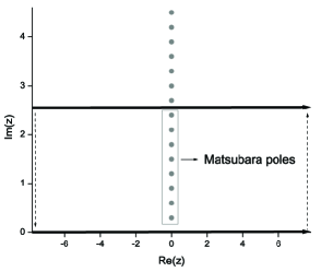
Figure 1: An illustrative plot showing the contour of integration for $f_{\alpha}(z)\Lambda_{\alpha}(z)$ with a single–Lorentzian spectral density of $\Omega_{1}=5$. The dots equidistantly distributing on ${\rm Re}(z)=0$ correspond to the Matsubara poles (grey dots) in the upper complex plane. Integration along the dark solid arrow lying right on the real axis gives the desired self–energy of Eq. (28). However, the resulting HEOM encounters numerical difficulties. Due to the fact that the two dark solid arrows form a closed loop (completed with the dark dashed arrows at infinitely distance carrying zero values), the self–energy can be obtained alternatively by summing up the residues at the poles within this loop.

As long as the modulus of $\bm{\Lambda}_{\alpha}(z)$ remains sufficiently small along the line ${\rm Im}(z)=y$, Eq. (34) presents a complementary contribution to the RHS of Eq. (31). The integration in Eq. (34) is transformed into summation of discrete terms, following the frequency dispersion scheme introduced in Sec. III.1, i.e., $\int_{{\rm Im}(z)=y}g(z)\,dz\rightarrow\sum_{q=1}^{N_{q}}w_{q}\,g(\epsilon_{q}+iy)$. We have thus

$$\tilde{\bm{\Sigma}}^{x,{\rm dev}}_{\alpha}(\tau-t)\simeq\sum_{q=1}^{N_{q}}\bm{K}^{x}_{\alpha q}e^{-\hat{\gamma}_{\alpha q}(t-\tau)},$$ (35)

with

$$\bm{K}^{x}_{\alpha q} =\varsigma_{x}i\,w_{q}f^{\varsigma_{x}}_{\alpha}(\epsilon_{q}+iy)\bm{\Lambda}_{\alpha}(\epsilon_{q}+iy),$$

$$\hat{\gamma}_{\alpha q} =-i(\epsilon_{q}+iy)=y-i\epsilon_{q}.$$ (36)

Therefore, overall $\tilde{\bm{\Sigma}}^{x}_{\alpha}(\tau-t)$ is given by combining the RHS of Eqs. (31) and (35). The total number of exponential functions is $N_{k}=N_{d}+N_{p}+N_{q}$. In practice, to make use of Eq. (35), one needs to assign an appropriate number of Matsubara terms, $N_{p}$. On one hand, a smaller $N_{p}$ leads to fewer unknown variables of HEOM. On the other hand, a too small $N_{p}$ (and hence a too small $y$) would cause severe convergence problem when solving the stationary solutions of HEOM. Therefore, the value of $N_{p}$ should be chosen carefully for the balance between computational cost and numerical difficulty. Once the $N_{p}$ and $y$ are settled, efficient quadratures can then be adopted to optimize the frequency dispersion (the set $\{w_{q},\epsilon_{q}\}$ with $q=1,\ldots,N_{q}$) for Eq. (34). Finally, all the $N_{d}$ poles of $\bm{\Lambda}_{\alpha}(z)$ inside the region $0<{\rm Im}(z)<y$ are collected.

It is important to note the value of $N_{d}$ depends on the mathematical form of basis functions, based on which $\bm{\Lambda}_{\alpha}(\epsilon)$ is expanded. The widely used multi–Lorentzian expansion has been adopted in Sec. III.2.1; see Eq. (29). Each Lorentzian function gives a pole in the upper complex plane. One of the advantages of using a Lorentzian function $g_{\rm L}(\epsilon)$ is that the magnitude of its analytically continued counterpart, $|g_{\rm L}(z)|$, decays smoothly as ${\rm Im}(z)$ increases. Therefore, the deviation term, $\tilde{\bm{\Sigma}}^{x,{\rm dev}}_{\alpha}(\tau-t)$ of Eq. (34), becomes consistently less significant as more Matsubara poles are considered explicitly. Alternative basis functions can also be used. For instance, a Gaussian function is analytic, and does not have any pole on the entire complex plane. Therefore, for $\bm{\Lambda}_{\alpha}(\epsilon)$ fitted by a number of Gaussian functions, $N_{d}=0$, which reduces the number of unknown variables of HEOM. However, care must be taken when treating the “deviation” contribution, as some of the $\bm{K}^{x}_{\alpha q}$ may assume large values, due to the nontrivial value of complex Gaussian function at certain $z=\epsilon_{q}+iy$.

Numerical tests on model systemsZhe09164708 have confirmed that as the temperature lowers, the total number of exponential functions needed to accurately resolve the self–energies in the hybrid scheme grows much slower than that in the Matsubara expansion scheme.

IV Approximate schemes for calculation of dissipation functional

IV.1 Schemes based on wide–band limit approximation

Even with the sophisticated hybrid scheme for decomposition of self–energies, the exact HEOM approach for the reduced electronic dynamics can still be expensive. Efficient approximate schemes are thus required. For clarity, we will omit the spin index in the following derivations of approximate schemes.

IV.1.1 TDDFT–NEGF–HEOM formalism under wide–band limit approximation

The wide–band limit (WBL) approximation involves the following assumptions for the electrodes: (i) their bandwidths are assumed to be infinitely large; and (ii) their linewidths are assumed to be energy–independent, i.e., $\bm{\Lambda}_{\alpha}(\epsilon)\approx\bm{\Lambda}_{\alpha}$. Denote $\tilde{\bm{\Lambda}}_{\alpha}\equiv\pi\bm{\Lambda}_{\alpha}$. From the definition of self–energies and the expansion of the Fermi function [Eq. (30) with $N_{p}\rightarrow+\infty$], one obtains for $t>\tau$

$$\bm{\Sigma}^{<,>}_{\alpha}(\tau,t) \equiv\pm i\,e^{i\int_{\tau}^{t}dt_{1}\Delta_{\alpha}(t_{1})}\int d\epsilon f^{\pm}_{\alpha}(\epsilon)\,e^{i\epsilon(t-\tau)}\bm{\Lambda}_{\alpha}(\epsilon)$$

$$=\pm i\delta(t-\tau)\tilde{\bm{\Lambda}}_{\alpha}$$

$$\quad+\frac{2}{\beta}\sum_{k=1}e^{i\int_{\tau}^{t}dt_{1}z_{\alpha k}(t_{1})}\tilde{\bm{\Lambda}}_{\alpha},$$ (37)

where $z_{\alpha k}(t)=z_{\alpha k}+\Delta_{\alpha}(t)$. The expansion of Fermi function thus leads to a sum of exponentials for the self–energies. We introduce auxiliary self–energies $\hat{\bm{\Sigma}}_{\alpha k}$ to account for the exponentials, i.e.,

$$\bm{\Sigma}^{<,>}_{\alpha}(\tau,t) =\pm i\delta(t-\tau)\tilde{\bm{\Lambda}}_{\alpha}+\sum_{k}\hat{\bm{\Sigma}}_{\alpha k}(\tau,t),$$ (38)

$$\hat{\bm{\Sigma}}_{\alpha k}(\tau,t) =\frac{2}{\beta}\,e^{i\int_{\tau}^{t}dt_{1}z_{\alpha k}(t_{1})}\tilde{\bm{\Lambda}}_{\alpha}.$$ (39)

It is implied that $\hat{\bm{\Sigma}}_{\alpha k}(t,t^{+})=\frac{2}{\beta}\tilde{\bm{\Lambda}}_{\alpha}$. Next, we insert relation Eq. (38) into Eq. (16), and arrive at

$$\bm{\varphi}_{\alpha}(t)=i\left[\bm{1}-2\bm{\sigma}_{\rm D}(t)\right]\tilde{\bm{\Lambda}}_{\alpha}+\sum_{k}\hat{\bm{\varphi}}_{\alpha k}(t),$$ (40)

with the auxiliary current matrices being as follows,

$$\hat{\bm{\varphi}}_{\alpha k}(t) =-i\int_{-\infty}^{t}d\tau\left[\bm{G}_{\rm D}^{<}(t,\tau)-\bm{G}_{\rm D}^{>}(t,\tau)\right]\hat{\bm{\Sigma}}_{\alpha k}(\tau,t)$$

$$=i\int_{-\infty}^{t}d\tau\,\bm{G}_{\rm D}^{r}(t,\tau)\,\hat{\bm{\Sigma}}_{\alpha k}(\tau,t).$$ (41)

Under the WBL approximation, NEGF formalism gives

$$\bm{G}_{\rm D}^{r}(t,\tau) =-i\vartheta(t-\tau)\,\bm{W}_{\rm D}^{-}(t)\,\bm{W}_{\rm D}^{+}(\tau),$$ (42)

$$\bm{W}_{\rm D}^{\pm}(t) =\exp_{\pm}\left\{\mp i\int_{0}^{t}dt_{1}\left[\bm{h}_{\rm D}(t_{1})-i\tilde{\bm{\Lambda}}\right]\right\}.$$ (43)

Here, we take the time from which the voltage emerges as $t_{0}=0$, i.e., $\Delta_{\alpha}(t\leq 0)=0$, and $\tilde{\bm{\Lambda}}=\sum_{\alpha}\tilde{\bm{\Lambda}}_{\alpha}$. Therefore, the EOM of $\hat{\bm{\varphi}}_{\alpha k}(t)$ can be established readily as follows,

$$\dot{\hat{\bm{\varphi}}}_{\alpha k}(t)=\frac{2}{\beta}\tilde{\bm{\Lambda}}_{\alpha}-i\left[\bm{h}_{\rm D}(t)-i\tilde{\bm{\Lambda}}-z_{\alpha k}(t)\right]\hat{\bm{\varphi}}_{\alpha k}(t).$$ (44)

The coupled equations of motion, Eqs. (4), (25), (40) and (44) can be solved together for a complete description of the nonequilibrium electronic dynamics of the device. Equation (44) is self–closed, which suggests that under the WBL approximation the TDDFT–HEOM automatically terminates at first tier, instead of second–tier termination for the exact formalism. Thus the additional second–tier auxiliary matricesJin08234703 are not needed with the WBL. Similar apporach has been adopted by Croy and Saalmann.croy

IV.1.2 TDDFT–NEGF–EOM formalism under adiabatic wide–band limit approximation

We consider another approximate scheme for $\bm{Q}_{\alpha}(t)$ based on WBL approximation for electrodes, as well as an adiabatic approximation for memory effect. The scheme aims at simplifying the TDDFT–NEGF formulation for $\bm{Q}_{\alpha}(t)$; see Eq. (8). Due to the WBL approximation, the ground/equilibrium–state self–energies become simply

$$\tilde{\bm{\Sigma}}^{a}_{\alpha}(\tau,t) =i\delta(t-\tau)\tilde{\bm{\Lambda}}_{\alpha},$$ (45)

$$\tilde{\bm{\Sigma}}^{<}_{\alpha}(\tau,t) =i\frac{1}{\pi}\left[\int_{-\infty}^{+\infty}f_{\alpha}(\epsilon)\,e^{i\epsilon(t-\tau)}\,d\epsilon\right]\tilde{\bm{\Lambda}}_{\alpha}.$$ (46)

By inserting Eqs. (45) and (46) into Eq. (8), the dissipation functional is formally simplified to be

$$\bm{Q}^{\rm AWBL}_{\alpha}(t) =\big{\{}\tilde{\bm{\Lambda}}_{\alpha},\bm{\sigma}_{\rm D}\big{\}}+\bm{P}_{\alpha}(t)+\left[\bm{P}_{\alpha}(t)\right]^{\dagger},$$ (47)

$$\bm{P}_{\alpha}(t) =-\int_{-\infty}^{+\infty}\bm{G}_{\rm D}^{r}(t,\tau)\bm{\Sigma}^{<}_{\alpha}(\tau,t)\,d\tau.$$ (48)

Before the external voltage is applied, the entire composite system is in its ground/equilibrium state. We have

$$\bm{P}_{\alpha}(t) =-\frac{i}{\pi}\,\bm{U}^{+}_{\alpha}(t)\Big{\{}\int_{-\infty}^{+\infty}f_{\alpha}(\epsilon)\Big{[}\frac{1}{\epsilon-\bm{h}_{\rm D}(0)+i\tilde{\bm{\Lambda}}}$$

$$\quad-i\int_{0}^{t}e^{-i\epsilon\tau}\bm{U}^{-}_{\alpha}(\tau)\,d\tau\Big{]}e^{i\epsilon t}d\epsilon\Big{\}}\tilde{\bm{\Lambda}}_{\alpha}.$$ (49)

$$\bm{U}^{\pm}_{\alpha}(t) \equiv\exp_{\pm}\Big{\{}\mp\!i\!\int_{0}^{t}d\tau\!\left[\bm{h}_{\rm D}(\tau)-i\tilde{\bm{\Lambda}}-\Delta_{\alpha}(\tau)\right]\Big{\}}.$$ (50)

To facilitate the calculation of $\bm{P}_{\alpha}(t)$ given by Eq. (49), an adiabatic approximation is adopt to evaluate the time integral within the square bracket on the RHS. The basic idea is to first disregard the time–dependence of $\bm{h}_{\rm D}(t)$ and $\Delta_{\alpha}(t)$ in Eq. (50), evaluate the time integral, and then restore subsequently the time–dependence of $\bm{h}_{\rm D}(t)$ and $\Delta_{\alpha}(t)$. The final approximated expression for $\bm{P}_{\alpha}(t)$ is as follows,

$$\bm{P}_{\alpha}(t) \simeq-\frac{i}{\pi}\bigg{\{}\bm{U}^{+}_{\alpha}(t)\int_{-\infty}^{+\infty}d\epsilon f_{\alpha}(\epsilon)\,e^{i\epsilon t}$$

$$\quad\times\left[\frac{1}{\epsilon-\bm{h}_{\rm D}(0)+i\tilde{\bm{\Lambda}}}-\frac{1}{\epsilon-\bm{h}_{\rm D}(t)+i\tilde{\bm{\Lambda}}+\Delta_{\alpha}(t)}\right]$$

$$\quad+\int_{-\infty}^{+\infty}\frac{f_{\alpha}(\epsilon)}{\epsilon-\bm{h}_{\rm D}(t)+i\tilde{\bm{\Lambda}}+\Delta_{\alpha}(t)}\,d\epsilon\bigg{\}}\,\tilde{\bm{\Lambda}}_{\alpha}.$$ (51)

The RHS of Eq. (51) gives exact $\bm{P}_{\alpha}(t)$ for the ground state at $t\leq 0$ and the steady state at $t\rightarrow+\infty$, provided that $\Delta_{\alpha}(t\rightarrow+\infty)$ is a constant. At $0<t<+\infty$, it provides an adiabatic connection between the ground and steady states. Equation (51) can be solved conveniently, along with the EOM for $\bm{U}^{+}_{\alpha}(t)$ as follows,

$$i\,\dot{\bm{U}}^{+}_{\alpha}(t)=\big{[}\bm{h}_{\rm D}(t)-i\tilde{\bm{\Lambda}}-\Delta_{\alpha}(t)\big{]}\,\bm{U}^{+}_{\alpha}(t).$$ (52)

IV.2 Scheme based on complete second–order quantum dissipation theory

As presented in Sec. III, the TDDFT–NEGF–HEOM for KS RSDM and associated auxiliary matrices terminate exactly at the second tier. This amounts to an explicit treatment of device–electrode interaction at leading $4$th–order.Jin08234703 The number of unknown matrices at zeroth, first, and second tier is $1$, $N_{\alpha}N_{k}$, and $N_{\alpha}^{2}N_{k}^{2}$, respectively. Here, $N_{k}$ is the number of exponential functions used to resolve the memory contents of self–energies or electrode correlation functions. Obviously, the second–tier variables dominate the computational cost for solving the TDDFT–NEGF–HEOM. Therefore, a straightforward way to reduce the computational expense is to avoid explicit involvement of the second–tier variables, i.e., to truncate the TDDFT–NEGF–HEOM at first tier approximately.

A simple truncation scheme is to set all second–tier auxiliary matrices to zero, i.e., $\bm{\varphi}_{\alpha k,\alpha^{\prime}k^{\prime}}(t)=\bm{0}$. This corresponds to the chronological ordering prescription of $2$nd–order QDT.

An alternative $2$nd–order approximation is as follows:

$$\bm{G}_{\rm D}^{<}(t,\tau) \approx i\,\bm{\sigma}_{\rm D}(t)\,\bm{U}_{\rm D}^{+}(t,\tau),$$

$$\bm{G}_{\rm D}^{>}(t,\tau) \approx-i\,\bar{\bm{\sigma}}_{\rm D}(t)\,\bm{U}_{\rm D}^{+}(t,\tau),$$ (53)

with

$$\bm{U}_{\rm D}^{\pm}(t,\tau)=\exp_{\pm}\Big{[}\mp i\int_{\tau}^{t}\bm{h}_{\rm D}(\zeta)\,d\zeta\Big{]}.$$ (54)

The dissipation functional becomes approximately

$$\bm{Q}_{\alpha}(t)\approx\left[\bm{\sigma}_{\rm D}(t)\,\bm{\Pi}^{>}_{\alpha}(t)+\bar{\bm{\sigma}}_{\rm D}(t)\,\bm{\Pi}^{<}_{\alpha}(t)+{\rm H.c.}\right],$$ (55)

where

$$\bm{\Pi}^{x}_{\alpha}(t) =i\int_{-\infty}^{t}d\tau\,\bm{U}_{\rm D}^{+}(t,\tau)\,\bm{\Sigma}^{x}_{\alpha}(\tau,t).$$ (56)

Following Sec. III, we decompose self–energies as linear combinations of exponential functions; see Eq. (24). This leads to

$$\bm{\Pi}^{x}_{\alpha}(t) =\sum_{k=1}^{N_{k}}\bm{\Pi}^{x}_{\alpha k}(t),$$

$$\bm{\Pi}^{x}_{\alpha k}(t) =i\int_{-\infty}^{t}d\tau\,\bm{U}_{\rm D}^{+}(t,\tau)\,\tilde{\bm{\Sigma}}^{x}_{\alpha k}(\tau-t)$$

$$\quad\times e^{i\int_{\tau}^{t}\Delta_{\alpha}(\zeta)d\zeta}.$$ (57)

The EOM for $\bm{\Pi}^{x}_{\alpha k}(t)$ is thus

$$i\,\dot{\bm{\Pi}}^{x}_{\alpha k}(t)=\left[\bm{h}_{\rm D}(t)-i\gamma_{\alpha k}-\Delta_{\alpha}(t)\right]\bm{\Pi}^{x}_{\alpha k}(t)-\bm{A}^{x}_{\alpha k},$$ (58)

with $\bm{A}^{x}_{\alpha k}$ and $\gamma_{\alpha k}$ referring to Eq. (24).

The resulting complete $2$nd–order QDT approach thus involves the coupled EOM for $\bm{\sigma}_{\rm D}(t)$ and $\{\bm{\Pi}^{x}_{\alpha k}(t)\}$, with the total number of unknown matrices being $N=2N_{\alpha}N_{k}+1$, much fewer than $N_{\alpha}^{2}N_{k}^{2}$ alone. This approach can be improved further, by formal inclusion of higher–order device–electrode interaction into the reduced system propagator $\bm{U}_{\rm D}^{+}(t,\tau)$. This can be achieved by attaching self–energy to $\bm{h}_{\rm D}(t)$ on the RHS of Eq. (54).

V Numerical results

As a test for our practical schemes, we have performed the numerical calculations employing the AWBL approximation as outlined in Sec. IV A.2. LODESTAR ldstar was used to carried out the calculations. The system of interest is a (5,5) carbon nanotube which is covalently bonded between two aluminum electrodes, as shown in Fig. 2. In the simulation box, we include a finite carbon nanotube and 32 aluminum atoms for each electrode explicitly. The minimum basis set STO–3G is adopted in the calculations. We simulate the time–dependent electric current through the left (right) electrode by taking the trace of the corresponding dissipative term $\bm{Q}_{\rm L}$ ($\bm{Q}_{\rm R}$); see Eq. (7).

Figure 3 shows the currents versus time for different numbers of carbon atoms, i.e. 20, 40, 60 and 80. The bias voltage $V_{b}$ is switched on exponentially at $t=0$, and as shown in Fig. 3. We observe that the currents reach their steady states in about 8 to 12 fs for different systems. Also, the value of the steady state current does not increase proportionally with the size of the carbon nanotube, as that of classical case. We note from Fig. 3 that the steady state currents for the systems with 20, 40, 60 and 80 carbon atoms are about 21, 9, 14 and 4 $\mu$A, respectively. This shows that the quantum finite size effect plays an important role at such small scales. We point out that all the above calculations are performed on single–CPU desktop personal computer, and the memory is 2 gigabytes.

VI Concluding remarks

We have proposed a first–principles TDDFT–NEGF–HEOM method for transient quantum transport through realistic electronic devices and structures. The TDDFT–NEGF–HEOM formalism is in principles exact, and formally equivalent to the TDDFT–NEGF–EOM formalism proposed previously. In practice, it involves hierarchical equations for KS RSDM of reduced system and associated auxiliary quantities.

By resolving memory contents of self–energies or electrode correlation functions, we construct QDT–HEOM in the KS reduced single–electron space. The resulting TDDFT–HEOM exactly terminate at the second–tier. TDDFT–NEGF–HEOM formalism combines TDDFT–NEGF–EOM and TDDFT–HEOM, and its computational cost is determined by the number of exponential functions used to expand the self–energies. Various decomposition schemes are presented.

To reduce computational cost further, we have also devised approximate schemes for TDDFT–NEGF–HEOM. One is based on the WBL treatment for self–energies. Another one is based on complete $2$nd–order QDT. These approximate schemes significantly reduce the computational cost, and improve the efficiency for solving the reduced electronic dynamics. Additional adiabatic approximation is introduced for the WBL scheme, and the resulting AWBL approximation turns out the most efficient scheme. Numerical simulations based on the AWBL scheme demonstrate that first–principles simulation can indeed be carried out for real devices, and the interesting results have been obtained.

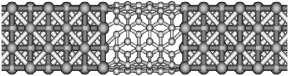
Figure 2: The ball–and–stick representation of the system of interest which is a carbon nanotube (5,5) welded to aluminium electrodes. There are 60 carbon atoms for the carbon nanotube in this case.

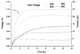
Figure 3: The grey solid line represents the bias voltage applied on the systems. The bias voltage is switched on exponentially, $V_{b}=V_{0}(1-e^{-t/a})$ with $V_{0}=0.1$ V and time constant $a=1$ fs. The transient currents for the systems with 20, 40, 60, 80 carbon atoms are shown dark dotted line, dashed line, solid line and dash-dot-dot line respectively.

Appendix A Detailed derivation of HEOM for an open noninteracting system

Here we give a direct derivation of HEOM for a noninteracting system, without resorting to the path–integral formalism for Fermion operators. Similarly with Ref. Jin08234703, , we introduce the reservoir $\hat{H}_{\rm B}$–interaction picture, where $\hat{H}_{\rm B}=\sum_{\alpha}\hat{H}_{\alpha}$. In this interaction picture, the total Hamiltonian is

$$\tilde{H}_{\rm T}(t)=H_{\rm D}+\sum_{\alpha}\tilde{H}_{\alpha{\rm D}}(t).$$ (59)

Here, $\tilde{H}_{\alpha{\rm D}}(t)=\sum_{\mu}\big{[}{\tilde{f}}^{\dagger}_{\alpha\mu}(t)a_{\mu}+a^{\dagger}_{\mu}{\tilde{f}}_{\alpha\mu}(t)\big{]}$ where ${\tilde{f}}^{\dagger}_{\alpha\mu}\left(t\right)=\sum_{k}\bm{t}_{\alpha k\mu}\,\tilde{d}^{\dagger}_{\alpha k}(t)$. The quantum Liouville equation reads

$$\dot{{\tilde{\rho}}}_{\rm T}(t) =-i\big{[}\tilde{H}_{\rm T}(t),\tilde{\rho}_{\rm T}(t)\big{]}$$

$$=-i{\cal L}_{\rm D}\,\tilde{\rho}_{\rm T}(t)-i\sum_{\alpha}{\cal L}_{\alpha{\rm D}}\,\tilde{\rho}_{\rm T}(t),$$ (60)

where the superoperators are defined as

$${\cal L}_{\rm D}~{}\cdot \equiv\left[H_{\rm D},\,\cdot\right],$$

$${\cal L}_{\alpha{\rm D}}~{}\cdot \equiv\big{[}\tilde{H}_{\alpha{\rm D}}(t),\,\cdot\big{]}.$$ (61)

First, we establish the EOM for the RSDM of primary interest, $\bm{\sigma}_{\rm D\mu\nu}(t)\equiv{\rm tr_{{}_{T}}}[a^{\dagger}_{\nu}a_{\mu}\rho_{\rm T}(t)]={\rm tr_{{}_{T}}}[a^{\dagger}_{\nu}a_{\mu}\tilde{\rho}_{\rm T}(t)]$. Following Eq. (A), we have

$$\quad i\dot{\bm{\sigma}}_{\rm D\mu\nu}(t)$$

$$={\rm tr_{{}_{T}}}[a^{\dagger}_{\nu}a_{\mu}\,{\cal L}_{\rm D}\,\tilde{\rho}_{\rm T}(t)]+\sum_{\alpha}{\rm tr_{{}_{T}}}[a^{\dagger}_{\nu}a_{\mu}\,{\cal L}_{\alpha{\rm D}}\,\tilde{\rho}_{\rm T}(t)]$$

$$={\rm tr_{{}_{T}}}\left\{\left[a^{\dagger}_{\nu}a_{\mu},H_{\rm D}\right]\tilde{\rho}_{\rm T}(t)\right\}$$

$$\quad+\sum_{\alpha}{\rm tr_{{}_{T}}}\big{\{}\big{[}a^{\dagger}_{\nu}a_{\mu},\tilde{H}_{\alpha{\rm D}}(t)\big{]}\tilde{\rho}_{\rm T}(t)\big{\}}$$

$$=\sum_{\mu^{\prime}\in{\rm D}}{\rm tr_{{}_{T}}}\big{[}\big{(}\bm{h}_{\rm D\mu\mu^{\prime}}a^{\dagger}_{\nu}a_{\mu^{\prime}}-\bm{h}_{\rm D\mu^{\prime}\nu}a^{\dagger}_{\mu^{\prime}}a_{\nu}\big{)}\tilde{\rho}_{\rm T}(t)\big{]}$$

$$\quad+\sum_{\alpha}\sum_{\mu^{\prime}\in{\rm D}}{\rm tr_{{}_{T}}}\Big{\{}\big{[}-{\tilde{f}}^{\dagger}_{\alpha\mu^{\prime}}(t)a_{\mu}\,{\delta}_{\nu\mu^{\prime}}$$

$$\qquad\qquad\qquad+a^{\dagger}_{\mu}{\tilde{f}}_{\alpha\mu^{\prime}}(t)\,\delta_{\mu\mu^{\prime}}\big{]}\,\tilde{\rho}_{\rm T}(t)\Big{\}}$$

$$=\left[\bm{h}_{\rm D},\bm{\sigma}_{\rm D}(t)\right]_{\mu\nu}-\sum_{\alpha}\big{[}\bm{\varphi}_{\alpha,\mu\nu}(t)-\bm{\varphi}^{\dagger}_{\alpha,\mu\nu}(t)\big{]}.$$ (62)

Here, the second equality results from trace cycling invariance property; and the fourth follows the definition of auxiliary RSDM, $\bm{\varphi}_{\alpha,\mu\nu}(t)\equiv{\rm tr_{{}_{T}}}[{\tilde{f}}^{\dagger}_{\alpha\nu}(t)\,a_{\mu}{\tilde{\rho}}_{\rm T}(t)]$, and its Hermitian conjugate $\bm{\varphi}^{\dagger}_{\alpha,\mu\nu}(t)={\rm tr_{{}_{T}}}[a^{\dagger}_{\nu}{\tilde{f}}_{\alpha\mu}(t){\tilde{\rho}}_{\rm T}(t)]$.

Considering the multiple–frequency–dispersed scheme in Ref. Jin08234703, , we can introduce the frequency dependence of $\tilde{f}$ and $\tilde{f}^{\dagger}$ from the beginning. In the reservoir $\hat{H}_{\rm B}$–interaction picture,

$$\dot{\tilde{d}}^{\dagger}_{\alpha k}(t) =-i\big{[}\tilde{d}^{\dagger}_{\alpha k}(t),\hat{H}_{\rm B}\big{]}$$

$$=i\left[\epsilon_{\alpha k}+\Delta_{\alpha}(t)\right]\tilde{d}^{\dagger}_{\alpha k}(t).$$ (63)

Simple integration leads to

$$\tilde{d}^{\dagger}_{\alpha k}(t) =e^{i\int_{t_{0}}^{t}\left[\epsilon_{\alpha k}+\Delta_{\alpha}(\tau)\right]d\tau}\,\tilde{d}^{\dagger}_{\alpha k},$$

$${\tilde{f}}^{\dagger}_{\alpha\mu}(t) =\sum_{k\in\alpha}\bm{t}_{\alpha k\mu}\,\tilde{d}^{\dagger}_{\alpha k}\,e^{i\int_{t_{0}}^{t}d\tau\left[\epsilon_{\alpha k}+\Delta_{\alpha}(\tau)\right]}$$

$$=\sum_{k\in\alpha}\int d\omega\,\delta(\omega-\epsilon_{\alpha k})\,e^{i\omega\left(t-t_{0}\right)}\,\bm{t}_{\alpha k\mu}\,\tilde{d}^{\dagger}_{\alpha k}$$

$$\quad\times e^{i\int_{t_{0}}^{t}d\tau\Delta_{\alpha}(\tau)}.$$ (64)

Let

$${\tilde{f}}^{\dagger}_{\alpha\mu}(\omega,t) =\sum_{k\in\alpha}\delta\left(\omega-\epsilon_{\alpha k}\right)e^{i\omega\left(t-t_{0}\right)}\,\bm{t}_{\alpha k\mu}\,\tilde{d}^{\dagger}_{\alpha k}$$

$$\quad\times e^{i\int_{t_{0}}^{t}d\tau\Delta_{\alpha}\left(\tau\right)},$$ (65)

we have ${\tilde{f}}^{\dagger}_{\alpha\mu}(t)=\int d\omega{\tilde{f}}^{\dagger}_{\alpha\mu}(\omega,t)$, ${\tilde{f}}_{\alpha\mu}(t)=\int d\omega{\tilde{f}}_{\alpha\mu}(\omega,t)$, and $\tilde{H}_{\alpha{\rm D}}(t)=\sum_{\mu}\int d\omega\big{[}{\tilde{f}}^{\dagger}_{\alpha\mu}(\omega,t)a_{\mu}+a^{\dagger}_{\mu}{\tilde{f}}_{\alpha\mu}(\omega,t)\big{]}$.

Define

$$\bm{\varphi}_{\alpha,\mu\nu}(\omega,t) \equiv{\rm tr_{{}_{T}}}\big{\{}\tilde{f}^{\dagger}_{\alpha\nu}(\omega,t)\,a_{\mu}\,{\tilde{\rho}}_{\rm T}(t)\big{\}},$$ (66)

$$\bm{\varphi}^{\dagger}_{\alpha,\mu\nu}(\omega,t) \equiv{\rm tr_{{}_{T}}}\big{\{}a^{\dagger}_{\nu}\,{\tilde{f}}_{\alpha\mu}(\omega,t)\,{\tilde{\rho}}_{\rm T}(t)\big{\}}.$$ (67)

They satisfy $\bm{\varphi}_{\alpha,\mu\nu}(t)=\int d\omega\,\bm{\varphi}_{\alpha,\mu\nu}(\omega,t)$ and $\bm{\varphi}^{\dagger}_{\alpha,\mu\nu}(t)=\int d\omega\,\bm{\varphi}^{\dagger}_{\alpha,\mu\nu}(\omega,t)$. Comparing with the NEGF formalism, it is readily verified that

$$\bm{\varphi}_{\alpha,\mu\nu}(\omega,t)=-i\sum_{k\in\alpha}\delta\left(\omega-\epsilon_{\alpha k}\right)\bm{G}^{<}_{\mu\alpha k}\left(t,t\right)\bm{t}_{\alpha k\nu}.$$ (68)

The following nonequilibrium Green’s function is defined on the Keldysh contour, where the time variable goes from $-\infty$ to $+\infty$ then back to $-\infty$:

$$\bm{G}_{\mu\alpha k}\left(\tau,\tau^{\prime}\right) \equiv-i\,{\rm tr_{{}_{T}}}\left\{T_{C}\big{[}a_{\mu}\left(\tau\right)d^{\dagger}_{\alpha k}\left(\tau^{\prime}\right)\big{]}\rho_{\rm T}\left(t_{0}\right)\right\}$$

$$=\sum_{\nu\in{\rm D}}\int_{C}d\tau_{1}\bm{G}_{\mu\nu}\left(\tau,\tau_{1}\right)\bm{t}^{*}_{\alpha k\nu}\,g_{\alpha k}\left(\tau_{1},\tau^{\prime}\right),$$ (69)

where the second equality follows the derivation for Eq. (B7) in Appendix B of Ref. Jauho, . With the Langreth’s analytic continuation rules,Langreth we have

$$\bm{G}^{<}_{\mu\alpha k}\left(t,t\right) =\sum_{\nu\in{\rm D}}\bm{t}^{*}_{\alpha k\nu}\int_{-\infty}^{\infty}dt_{1}\left[\bm{G}^{r}_{\mu\nu}\left(t,t_{1}\right)g^{<}_{\alpha k}\left(t_{1},t\right)\right.$$

$$\quad\left.+\,\bm{G}^{<}_{\mu\nu}\left(t,t_{1}\right)g^{a}_{\alpha k}\left(t_{1},t\right)\right].$$ (70)

Inserting Eq. (70) into Eq. (68) leads to

$$\bm{\varphi}_{\alpha,\mu\nu}(\omega,t) =-i\sum_{k\in\alpha}\sum_{\nu^{\prime}\in{\rm D}}\bm{t}^{*}_{\alpha k\nu^{\prime}}\,\bm{t}_{\alpha k\nu}\,\delta(\omega-\epsilon_{\alpha k})\int_{-\infty}^{\infty}dt_{1}\left[\bm{G}^{r}_{\mu\nu^{\prime}}(t,t_{1})\,g^{<}_{\alpha k}(t_{1},t)+\bm{G}^{<}_{\mu\nu^{\prime}}(t,t_{1})\,g^{a}_{\alpha k}(t_{1},t)\right]$$

$$=-i\sum_{\nu^{\prime}\in{\rm D}}\int_{-\infty}^{\infty}dt_{1}\left[\bm{G}^{r}_{\mu\nu^{\prime}}\left(t,t_{1}\right)\bm{\Sigma}^{<}_{\alpha,\nu^{\prime}\nu}\left(t_{1},t;\omega\right)+\bm{G}^{<}_{\mu\nu^{\prime}}\left(t,t_{1}\right)\bm{\Sigma}^{a}_{\alpha,\nu^{\prime}\nu}\left(t_{1},t;\omega\right)\right]$$

$$=i\sum_{\nu^{\prime}\in{\rm D}}\int_{-\infty}^{t}dt_{1}\left[\bm{G}^{<}_{\mu\nu^{\prime}}\left(t,t_{1}\right)\bm{\Sigma}^{>}_{\alpha,\nu^{\prime}\nu}\left(t_{1},t;\omega\right)-\bm{G}^{>}_{\mu\nu^{\prime}}\left(t,t_{1}\right)\bm{\Sigma}^{<}_{\alpha,\nu^{\prime}\nu}\left(t_{1},t;\omega\right)\right],$$ (71)

where the third equality employs the relation

$$\bm{X}^{r,a}\left(t,\tau\right)=\pm\vartheta\left[\pm\left(t-\tau\right)\right]\left[\bm{X}^{>}(t,\tau)-\bm{X}^{<}(t,\tau)\right]$$ (72)

with $\bm{X}$ being $\bm{G}_{\rm D}$ or $\bm{\Sigma}_{\alpha}$. The frequency dispersed self–energies are defined by

$$\bm{\Sigma}^{x}_{\alpha,\nu^{\prime}\nu}(t_{1},t;\omega)\equiv\sum_{k\in\alpha}\bm{t}^{*}_{\alpha k\nu^{\prime}}\bm{t}_{\alpha k\nu}\,\delta(\omega-\epsilon_{\alpha k})\,g^{x}_{\alpha k}(t_{1},t),$$ (73)

where $x=r$, $a$, $<$, and $>$. They satisfy

$$\bm{\Sigma}^{<}_{\alpha,\nu^{\prime}\nu}(t_{1},t) =\int d\omega\,\bm{\Sigma}^{<}_{\alpha,\nu^{\prime}\nu}(t_{1},t;\omega)$$

$$=i\sum_{k\in\alpha}\bm{t}^{*}_{\alpha k\nu^{\prime}}\bm{t}_{\alpha k\nu}\int d\omega\,\delta(\omega-\epsilon_{\alpha k})f_{\alpha}\left(\epsilon_{\alpha k}\right)$$

$$\quad\times e^{i\omega\left(t-t_{1}\right)}e^{i\int_{t_{1}}^{t}d\tau\Delta_{\alpha}\left(\tau\right)}$$

$$=i\int d\omega\,\bm{\Lambda}_{\alpha,\nu^{\prime}\nu}(\omega)f_{\alpha}(\omega)\,e^{i\omega\left(t-t_{1}\right)}$$

$$\quad\times e^{i\int_{t_{1}}^{t}d\tau\Delta_{\alpha}\left(\tau\right)}.$$ (74)

Next, we establish the EOM for the first–tier auxiliary RSDM, $\bm{\varphi}_{\alpha,\mu\nu}(\omega,t)$, as follows,

$$\qquad{\dot{\bm{\varphi}}}_{\alpha,\mu\nu}(\omega,t)$$

$$={\rm tr_{{}_{T}}}\big{\{}\dot{\tilde{f}}^{\dagger}_{\alpha\nu}(\omega,t)\,a_{\mu}\,{\tilde{\rho}}_{\rm T}(t)+\tilde{f}^{\dagger}_{\alpha\nu}(\omega,t)a_{\mu}\,{\dot{\tilde{\rho}}}_{\rm T}(t)\big{\}}$$

$$=i\left[\omega+\Delta_{\alpha}(t)\right]\bm{\varphi}_{\alpha,\mu\nu}(\omega,t)$$

$$\quad+{\rm tr_{{}_{T}}}\big{\{}\tilde{f}^{\dagger}_{\alpha\nu}(\omega,t)\,a_{\mu}\big{[}-i{\cal L}_{\rm D}\,{\tilde{\rho}}_{\rm T}(t)\big{]}\big{\}}$$

$$\quad+\sum_{\alpha^{\prime}}{\rm tr_{{}_{T}}}\big{\{}\tilde{f}^{\dagger}_{\alpha\nu}(\omega,t)\,a_{\mu}\big{[}-i{\cal L}_{\alpha^{\prime}\rm D}\,{\tilde{\rho}}_{\rm T}(t)\big{]}\big{\}}$$

$$=i\left[\omega+\Delta_{\alpha}(t)\right]\bm{\varphi}_{\alpha,\mu\nu}(\omega,t)$$

$$\quad-i\,{\rm tr_{{}_{T}}}\big{\{}\big{[}\tilde{f}^{\dagger}_{\alpha\nu}(\omega,t)\,a_{\mu},H_{\rm D}\big{]}\tilde{\rho}_{\rm T}(t)\big{\}}$$

$$\quad-i\sum_{\alpha^{\prime}}{\rm tr_{{}_{T}}}\big{\{}\big{[}\tilde{f}^{\dagger}_{\alpha\nu}(\omega,t)\,a_{\mu},\tilde{H}_{\alpha^{\prime}{\rm D}}(t)\big{]}\tilde{\rho}_{\rm T}(t)\big{\}}$$

$$=i\left[\omega+\Delta_{\alpha}(t)\right]\bm{\varphi}_{\alpha,\mu\nu}(\omega,t)$$

$$\quad-i\sum_{\mu^{\prime}\in{\rm D}}\bm{h}_{\rm D\mu\mu^{\prime}}\,{\rm tr_{{}_{T}}}\big{\{}\tilde{f}^{\dagger}_{\alpha\nu}(\omega,t)\,a_{\mu^{\prime}}\,\tilde{\rho}_{\rm T}(t)\big{\}}$$

$$\quad-i\sum_{\alpha^{\prime}}\int d\omega^{\prime}{\rm tr_{{}_{T}}}\big{\{}\tilde{f}^{\dagger}_{\alpha\nu}(\omega,t)\,\tilde{f}_{\alpha^{\prime}\mu}(\omega^{\prime},t)\,\tilde{\rho}_{\rm T}(t)\big{\}}$$

$$\quad+i\sum_{k\in\alpha}\sum_{\mu^{\prime}\in{\rm D}}{\rm tr_{{}_{T}}}\big{\{}\bm{t}_{\alpha k\nu}\,\bm{t}^{*}_{\alpha k\mu^{\prime}}\delta(\omega-\epsilon_{\alpha k})\,a^{\dagger}_{\mu^{\prime}}\,a_{\mu}\,\tilde{\rho}_{\rm T}(t)\big{\}}$$

$$=i\left[\omega+\Delta_{\alpha}(t)\right]\bm{\varphi}_{\alpha,\mu\nu}(\omega,t)$$

$$\quad-i\sum_{\mu^{\prime}\in{\rm D}}\big{[}\bm{h}_{\rm D\mu\mu^{\prime}}\,\bm{\varphi}_{\alpha,\mu^{\prime}\nu}(\omega,t)-\bm{\sigma}_{\mu\mu^{\prime}}(t)\,\bm{\Lambda}_{\alpha,\mu^{\prime}\nu}(\omega)\big{]}$$

$$\quad-i\sum_{\alpha^{\prime}}\int d\omega^{\prime}\,{\rm tr_{{}_{T}}}\big{\{}\tilde{f}^{\dagger}_{\alpha\nu}(\omega,t)\,\tilde{f}_{\alpha^{\prime}\mu}(\omega^{\prime},t)\,\tilde{\rho}_{\rm T}(t)\big{\}}.$$ (75)

Comparing with the NEGF formalism, it is readily verified that

$$\qquad{\rm tr_{{}_{T}}}\big{\{}\tilde{f}^{\dagger}_{\alpha\nu}(\omega,t)\,\tilde{f}_{\alpha^{\prime}\mu}(\omega^{\prime},t)\,\tilde{\rho}_{\rm T}(t)\big{\}}$$

$$=\sum_{k\in\alpha}\sum_{k^{\prime}\in\alpha^{\prime}}\delta(\omega-\epsilon_{\alpha k})\,\delta(\omega^{\prime}-\epsilon_{\alpha^{\prime}k^{\prime}})\,\bm{t}_{\alpha k\nu}\bm{t}^{*}_{\alpha^{\prime}k^{\prime}\mu}$$

$$\qquad\times{\rm tr_{{}_{T}}}\big{\{}\tilde{d}^{\dagger}_{\alpha k}\,\tilde{d}_{\alpha^{\prime}k^{\prime}}\,\tilde{\rho}_{\rm T}(t)\big{\}}$$

$$=-i\sum_{k\in\alpha}\sum_{k^{\prime}\in\alpha^{\prime}}\delta(\omega-\epsilon_{\alpha k})\,\delta(\omega^{\prime}-\epsilon_{\alpha^{\prime}k^{\prime}})\,\bm{t}_{\alpha k\nu}\bm{t}^{*}_{\alpha^{\prime}k^{\prime}\mu}$$

$$\qquad\times\bm{G}^{<}_{\alpha^{\prime}k^{\prime},\alpha k}(t,t).$$ (76)

Generally, the NEGF on the same Keldysh contour satisfies

$$\bm{G}_{\alpha^{\prime}k^{\prime},\alpha k}\left(\tau,\tau^{\prime}\right) =-i\,{\rm tr_{{}_{T}}}\big{\{}T_{C}\big{[}d_{\alpha^{\prime}k^{\prime}}(\tau)\,d^{\dagger}_{\alpha k}(\tau^{\prime})\big{]}\rho_{\rm T}(t_{0})\big{\}}$$

$$=\delta_{\alpha\alpha^{\prime}}\delta_{kk^{\prime}}\,g_{\alpha k}(\tau,\tau^{\prime})$$

$$\quad+\sum_{\mu_{1}\mu_{2}\in{\rm D}}\int_{C}d\tau_{1}\int_{C}d\tau_{2}\,g_{\alpha^{\prime}k^{\prime}}\left(\tau,\tau_{1}\right)\bm{t}_{\alpha^{\prime}k^{\prime}\mu_{1}}$$

$$\quad\times\bm{G}_{\mu_{1}\mu_{2}}\left(\tau_{1},\tau_{2}\right)\,\bm{t}^{*}_{\alpha k\mu_{2}}\,g_{\alpha k}\left(\tau_{2},\tau^{\prime}\right),$$ (77)

where the same technique in Ref. Jauho, adopted for derivation of Eq. (69) is used. At $\tau=\tau^{\prime}=t$ the lesser component of Green’s function for the uncoupled lead is $g^{<}_{\alpha k}\left(t,t\right)=g^{<}_{\alpha k}(t-t)=if_{\alpha}\left(\epsilon_{\alpha k}\right)$. Inserting the first term on RHS of Eq. (A) into Eq. (A) leads to

$$\quad-i\,\sum_{\alpha^{\prime}}\sum_{k\in\alpha}\sum_{k^{\prime}\in\alpha^{\prime}}\int d\omega^{\prime}\,\delta(\omega-\epsilon_{\alpha k})\,\delta(\omega^{\prime}-\epsilon_{\alpha^{\prime}k^{\prime}})$$

$$\qquad\qquad\qquad\qquad\times\bm{t}_{\alpha k\nu}\,\bm{t}^{*}_{\alpha^{\prime}k^{\prime}\mu}\delta_{\alpha\alpha^{\prime}}\delta_{kk^{\prime}}\,\big{[}if_{\alpha}\left(\epsilon_{\alpha k}\right)\big{]}$$

$$=\bm{\Lambda}_{\alpha,\mu\nu}(\omega)\,f_{\alpha}(\omega).$$ (78)

Inserting the second term on RHS of Eq. (A) into Eq. (A) while using Eq. (73), we arrive at a term on the RHS of Eq. (75)

$$\bm{\varphi}_{\alpha\alpha^{\prime},\nu\mu}(\omega,\omega^{\prime},t) =-i\!\!\sum_{\mu_{1}\mu_{2}\in{\rm D}}\int_{C}d\tau_{1}\int_{C}d\tau_{2}\big{[}\bm{\Sigma}_{\alpha^{\prime},\mu\mu_{1}}(t,\tau_{1};\omega^{\prime})$$

$$\times\bm{G}_{\mu_{1}\mu_{2}}(\tau_{1},\tau_{2})\bm{\Sigma}_{\alpha,\mu_{2}\nu}(\tau_{2},t;\omega)\big{]}^{<}.$$ (79)

It turns out that the EOM for the first–tier auxiliary RSDM, $\bm{\varphi}_{\alpha,\mu\nu}(\omega,t)$, is formally identical to that given by path–integral formulation in Ref. Jin08234703, . Combining Eqs. (A) through (79), Eq. (75) finally reads:

$$i{\dot{\bm{\varphi}}}_{\alpha,\mu\nu}(\omega,t) =-\left[\omega+\Delta_{\alpha}(t)\right]\bm{\varphi}_{\alpha,\mu\nu}(\omega,t)$$

$$\quad+\sum_{\mu^{\prime}\in{\rm D}}\bm{h}_{\rm D\mu\mu^{\prime}}\bm{\varphi}_{\alpha,\mu^{\prime}\nu}(\omega,t)$$

$$\quad-\sum_{\mu^{\prime}\in{\rm D}}\bm{\sigma}_{\rm D\mu\mu^{\prime}}(t)\bm{\Lambda}_{\alpha,\mu^{\prime}\nu}(\omega)+f_{\alpha}(\omega)\bm{\Lambda}_{\alpha,\mu\nu}(\omega)$$

$$\quad+\sum_{\alpha^{\prime}}\int d\omega^{\prime}\,\bm{\varphi}_{\alpha\alpha^{\prime},\nu\mu}(\omega,\omega^{\prime},t).$$ (80)

Here the compact definition (79) establishes the natural connection between the second–tier auxiliary RSDM and NEGF quantities. Again, using the Langreth’s analytic continuation rules,Langreth we can immediately write down a real time expression for Eq. (79) as follows, which looks however more complicated.

$$\quad\bm{\varphi}_{\alpha\alpha^{\prime},\nu\mu}(\omega,\omega^{\prime},t)$$

$$=i\sum_{\mu_{1}\mu_{2}\in{\rm D}}\bigg{\{}\int_{-\infty}^{t}dt_{2}\,\bigg{[}\int_{C}d\tau_{1}\,\bm{\Sigma}_{\alpha^{\prime},\mu\mu_{1}}(t,\tau_{1};\omega^{\prime})\,\bm{G}_{\mu_{1}\mu_{2}}(\tau_{1},t_{2})\bigg{]}^{<}\,\bm{\Sigma}^{>}_{\alpha,\mu_{2}\nu}(t_{2},t;\omega)$$

$$\qquad\quad-\int_{-\infty}^{t}dt_{2}\,\bigg{[}\int_{C}d\tau_{1}\bm{\Sigma}_{\alpha^{\prime},\mu\mu_{1}}(t,\tau_{1};\omega^{\prime})\bm{G}_{\mu_{1}\mu_{2}}(\tau_{1},t_{2})\bigg{]}^{>}\,\bm{\Sigma}^{<}_{\alpha,\mu_{2}\nu}(t_{2},t;\omega)\bigg{\}}$$

$$=i\sum_{\mu_{1}\mu_{2}\in{\rm D}}\bigg{\{}\int_{-\infty}^{t}dt_{2}\int_{-\infty}^{t}dt_{1}\left[\bm{\Sigma}^{<}_{\alpha^{\prime},\mu\mu_{1}}(t,t_{1};\omega^{\prime})\bm{G}^{a}_{\mu_{1}\mu_{2}}(t_{1},t_{2})+\bm{\Sigma}^{r}_{\alpha^{\prime},\mu\mu_{1}}(t,t_{1};\omega^{\prime})\bm{G}^{<}_{\mu_{1}\mu_{2}}(t_{1},t_{2})\right]\,\bm{\Sigma}^{>}_{\alpha,\mu_{2}\nu}(t_{2},t;\omega)$$

$$\qquad\quad-\int_{-\infty}^{t}dt_{2}\int_{-\infty}^{t}dt_{1}\left[\bm{\Sigma}^{r}_{\alpha^{\prime},\mu\mu_{1}}(t,t_{1};\omega^{\prime})\bm{G}^{>}_{\mu_{1}\mu_{2}}(t_{1},t_{2})+\bm{\Sigma}^{>}_{\alpha^{\prime},\mu\mu_{1}}(t,t_{1};\omega^{\prime})\bm{G}^{a}_{\mu_{1}\mu_{2}}(t_{1},t_{2})\right]\,\bm{\Sigma}^{<}_{\alpha,\mu_{2}\nu}(t_{2},t;\omega)\bigg{\}}.$$ (81)

The last equality recovers Eqs. (22) and (24) in Ref. croy2, . At $t\rightarrow-\infty$ the device and leads are fully decoupled, i.e. $\tilde{\rho}_{\rm T}(-\infty)=\rho_{\rm B}\otimes\tilde{\rho}_{\rm D}(-\infty)$. Noting that

$$\quad\bm{\Lambda}_{\alpha,\mu\nu}(\omega)f_{\alpha}(\omega)$$

$$=\int d\omega^{\prime}\,{\rm tr_{{}_{T}}}\big{[}\tilde{f}^{\dagger}_{\alpha\nu}(\omega,t)\tilde{f}_{\alpha^{\prime}\mu}(\omega^{\prime},t)\,\tilde{\rho}_{\rm T}(-\infty)\big{]},$$ (82)

we can have a most simple and compact expression of the second–tier auxiliary RSDM as follows,

$$\quad\bm{\varphi}_{\alpha\alpha^{\prime},\nu\mu}(\omega,\omega^{\prime},t)$$

$$={\rm tr_{{}_{T}}}\big{\{}\tilde{f}^{\dagger}_{\alpha\nu}(\omega,t)\,\tilde{f}_{\alpha^{\prime}\mu}(\omega^{\prime},t)\left[\tilde{\rho}_{\rm T}(t)-\tilde{\rho}_{\rm T}(-\infty)\right]\big{\}}.$$ (83)

Based on Eq. (83), it is easier to obtain the EOM for the second–tier auxiliary RSDM, $\bm{\varphi}_{\alpha\alpha^{\prime},\nu\mu}(\omega,\omega^{\prime},t)$, as follows.

$$\quad\dot{\bm{\varphi}}_{\alpha\alpha^{\prime},\nu\mu}(\omega,\omega^{\prime},t)$$

$$=i\left[\omega+\Delta_{\alpha}(t)\right]\bm{\varphi}_{\alpha\alpha^{\prime},\nu\mu}(\omega,\omega^{\prime},t)-i\left[\omega^{\prime}+\Delta_{\alpha^{\prime}}(t)\right]\bm{\varphi}_{\alpha\alpha^{\prime},\nu\mu}(\omega,\omega^{\prime},t)+{\rm tr_{{}_{T}}}\big{[}\tilde{f}^{\dagger}_{\alpha\nu}(\omega,t)\,\tilde{f}_{\alpha^{\prime}\mu}(\omega^{\prime},t)\,\dot{\tilde{\rho}}_{\rm T}(t)\big{]}$$

$$=i\left[\omega+\Delta_{\alpha}(t)-\omega^{\prime}-\Delta_{\alpha^{\prime}}(t)\right]\bm{\varphi}_{\alpha\alpha^{\prime},\nu\mu}(\omega,\omega^{\prime},t)+{\rm tr_{{}_{T}}}\big{\{}\tilde{f}^{\dagger}_{\alpha\nu}(\omega,t)\,\tilde{f}_{\alpha^{\prime}\mu}(\omega^{\prime},t)\,\left[-i{\cal L}_{\rm D}\,\tilde{\rho}_{\rm T}(t)\right]\big{\}}$$

$$\quad+\sum_{\alpha_{1}}{\rm tr_{{}_{T}}}\big{\{}\tilde{f}^{\dagger}_{\alpha\nu}(\omega,t)\tilde{f}_{\alpha^{\prime}\mu}\left(\omega^{\prime},t\right)\,\left[-i{\cal L}_{\alpha_{1}{\rm D}}\,\tilde{\rho}_{\rm T}(t)\right]\big{\}}$$

$$=i\left[\omega+\Delta_{\alpha}(t)-\omega^{\prime}-\Delta_{\alpha^{\prime}}(t)\right]\bm{\varphi}_{\alpha\alpha^{\prime},\nu\mu}(\omega,\omega^{\prime},t)-i\,{\rm tr_{{}_{T}}}\big{\{}\big{[}\tilde{f}^{\dagger}_{\alpha\nu}(\omega,t)\,\tilde{f}_{\alpha^{\prime}\mu}(\omega^{\prime},t),H_{\rm D}\big{]}\tilde{\rho}_{\rm T}(t)\big{\}}$$

$$\quad-i\sum_{\alpha_{1}}{\rm tr_{{}_{T}}}\big{\{}\big{[}\tilde{f}^{\dagger}_{\alpha\nu}(\omega,t)\,\tilde{f}_{\alpha^{\prime}\mu}\left(\omega^{\prime},t\right),\tilde{H}_{\alpha^{\prime}{\rm D}}(t)\big{]}\,\tilde{\rho}_{\rm T}(t)\big{\}}$$

$$=i\left[\omega+\Delta_{\alpha}(t)-\omega^{\prime}-\Delta_{\alpha^{\prime}}(t)\right]\bm{\varphi}_{\alpha\alpha^{\prime},\nu\mu}(\omega,\omega^{\prime},t)$$

$$\quad-i\sum_{\alpha_{1}}\sum_{\mu^{\prime}\in{\rm D}}\sum_{k_{1}\in\alpha_{1}}\sum_{k^{\prime}\in\alpha^{\prime}}{\rm tr_{{}_{T}}}\big{[}\tilde{f}^{\dagger}_{\alpha\nu}\left(\omega,t\right)a_{\mu^{\prime}}\delta_{\alpha^{\prime}\alpha_{1}}\delta_{k^{\prime}k_{1}}\delta(\omega^{\prime}-\epsilon_{\alpha^{\prime}k^{\prime}})\,\bm{t}_{\alpha_{1}k_{1}\mu^{\prime}}\,\bm{t}^{*}_{\alpha^{\prime}k^{\prime}\mu}\,\tilde{\rho}_{\rm T}(t)\big{]}$$

$$\quad+i\sum_{\alpha_{1}}\sum_{\mu^{\prime}\in{\rm D}}\sum_{k_{1}\in\alpha_{1}}\sum_{k\in\alpha}{\rm tr_{{}_{T}}}\big{[}a^{\dagger}_{\mu^{\prime}}\tilde{f}_{\alpha\mu}(\omega^{\prime},t)\,\delta_{\alpha\alpha_{1}}\delta_{kk_{1}}\delta(\omega-\epsilon_{\alpha k})\,\bm{t}_{\alpha_{1}k_{1}\nu}\,\bm{t}^{*}_{\alpha k\mu^{\prime}}\,\tilde{\rho}_{\rm T}(t)\big{]}$$

$$=i\left[\omega+\Delta_{\alpha}(t)-\omega^{\prime}-\Delta_{\alpha^{\prime}}(t)\right]\bm{\varphi}_{\alpha\alpha^{\prime},\nu\mu}(\omega,\omega^{\prime},t)-i\sum_{\mu^{\prime}\in{\rm D}}\bm{\Lambda}_{\alpha^{\prime},\mu\mu^{\prime}}(\omega^{\prime})\bm{\varphi}_{\alpha,\mu^{\prime}\nu}(\omega,t)+i\sum_{\mu^{\prime}\in{\rm D}}\bm{\varphi}^{\dagger}_{\alpha^{\prime},\mu\mu^{\prime}}(\omega^{\prime},t)\bm{\Lambda}_{\alpha,\mu^{\prime}\nu}(\omega).$$ (84)

The last equality recovers Eq. (6.6) in Ref. Jin08234703, .

Appendix B Remarks on Landauer–Büttiker formula for steady current

Under an external voltage applied to electrode $\alpha$, a homogeneous energy shift $\Delta_{\alpha}$ is resulted for all energy levels, and the self–energy is thus

$$\bm{\Sigma}^{x}_{\alpha}(t,\tau)=\exp\left[-i\int_{\tau}^{t}\Delta_{\alpha}(\zeta)d\zeta\right]\tilde{\bm{\Sigma}}^{x}_{\alpha}(t-\tau),$$ (85)

where $x=r,a,<$, and $>$; and the tilde symbol denotes quantities of ground/equilibrium–state in absence of any voltage, where translational invariance in time applies.

For the composite system to approach a steady state as $t\rightarrow+\infty$, it is necessary to have $\Delta_{\alpha}^{\infty}\equiv\Delta_{\alpha}(t\rightarrow+\infty)$ approaching a constant for any $\alpha$. Based on Riemann–Lebesgue lemma, $\bm{G}_{\rm D}(t,\tau)=\bm{\Sigma}_{\alpha}(t,\tau)=0$ as $t\rightarrow+\infty$ and $\tau$ remains finite. For $t,\tau\rightarrow+\infty$, $\bm{G}_{\rm D}(t,\tau)=\bm{G}_{\rm D}(t-\tau)$ and $\bm{\Sigma}_{\alpha}(t,\tau)=\bm{\Sigma}_{\alpha}(t-\tau)$, i.e., translation invariance in time is retrieved at steady state.

The NEGF formalism gives steady current through electrode $\alpha$, $J_{\alpha}^{\infty}\equiv J_{\alpha}(t\rightarrow+\infty)$, as follows,

$$J_{\alpha}^{\infty} =-{\rm tr}_{\rm D}\left[\bm{Q}_{\alpha}(t\rightarrow+\infty)\right]$$

$$=\sum_{\alpha^{\prime}\neq\alpha}\int d\epsilon\left[f_{\alpha}(\epsilon)-f_{\alpha^{\prime}}(\epsilon)\right]T_{\alpha\alpha^{\prime}}(\epsilon),$$ (86)

$$T_{\alpha\alpha^{\prime}}(\epsilon) =2\pi\,{\rm tr}_{\rm D}\Big{[}\bm{G}_{\rm D}^{r}(\epsilon)\bm{\Lambda}_{\alpha^{\prime}}(\epsilon^{\infty}_{\alpha^{\prime}})\bm{G}_{\rm D}^{a}(\epsilon)\bm{\Lambda}_{\alpha}(\epsilon^{\infty}_{\alpha})\Big{]}.$$ (87)

Here, $\epsilon^{\infty}_{\alpha}\equiv\epsilon-\Delta^{\infty}_{\alpha}$, and $T_{\alpha\alpha^{\prime}}(\epsilon)$ is the KS transmission coefficient between electrodes $\alpha$ and $\alpha^{\prime}$. Equations (86) and (87) correspond formally to the Landauer–Büttiker formula. Equation (86) has also been reached in the framework of HEOM–QDT, see Ref. Jin08234703, . It is worth emphasizing that the exact XC potential of TDDFT is in principle frequency–dependent.

Equations (86) and (87) have been widely employed in the DFT–NEGF approach to simulate steady current through molecular devices and structures. The exact XC potential may depend explicitly on the time evolution history of electron density in TDDFT, while it is determined exclusively by $\rho(\bm{r},t\rightarrow+\infty)$ in stationary DFT. Under the same time–dependent applied voltage, DFT and TDDFT frameworks result in explicitly different steady current if and only if a nonadiabatic (or frequency–dependent) XC potential is adopted in TDDFT framework. In other words, DFT–NEGF approach is regarded as an adiabatic version of TDDFT–NEGF.

In principle, the steady current may also vary upon different time–dependent applied voltages, even if the voltage amplitudes are same at $t\to+\infty$. For instance, there may be multiple steady states corresponding to the multiple stationary solutions of the TDDFT–EOM, Eq. (6). The actual steady state reached at $t\to+\infty$ is thus completely determined by the initial electron density, and the history of externally applied voltage.

It has been shown that bound states in the device region would give rise to persistent oscillating current across the device–electrode interfaces.Ste07195115 ; Kho094535 In such cases, the Landauer–Büttiker formula becomes inadequate for describing the long–time limit of transient current. In fact, these bound states are physically decoupled with the rest of composite system, and form an isolated subsystem. When this isolated subsystem possesses nontrivial component (such as tail of wavefunction) inside the $\bm{r}$–space of electrodes, the persistent oscillating current would arise, as an electron transfers across the device–electrode interfaces, but remains within the subsystem. It is thus inferred that the magnitude of oscillating current would diminish as the device region is enlarged by pushing the interfaces (where the currents are measured) deeper into the electrodes. The oscillating current would vanish completely with all the bound states fully accommodated in the device region.

References

- (1) E. Runge and E. K. U. Gross, Phys. Rev. Lett. 52, 997 (1984).
- (2) G. Stefanucci and C.-O. Almbladh, Europhys. Lett. 67, 14 (2004); G. Stefanucci and C.-O. Almbladh, Phys. Rev. B 69, 195318 (2004).
- (3) S. Kurth, G. Stefanucci, C.-O. Almbladh, A. Rubio, and E. K. U. Gross, Phys. Rev. B 72, 035308 (2005).
- (4) X. Zheng and G. H. Chen, arXiv:physics/0502021; C. Y. Yam, X. Zheng, and G. H. Chen, J. Comput. Theor. Nanosci. 3, 857 (2006).
- (5) X. Zheng, F. Wang, and G. H. Chen, arXiv:quant-ph/0606169; G. H. Chen, in Recent Progress in Computational Sciences and Engineering, edited by T. Simos and G. Maroulis, Lecture Series on Computer and Computational Sciences Vol. 7 Brill, Leiden, 2006, p. 803.
- (6) X. Zheng, F. Wang, C. Y. Yam, Y. Mo, and G. H. Chen, Phys. Rev. B 75, 195127 (2007).
- (7) C. Y. Yam, Y. Mo, F. Wang, X. B. Li, G. H. Chen, X. Zheng, Y. Matsuda, J. Tahir-Kheli, and W. A. Goddard III, Nanotechnology 19, 495203 (2008).
- (8) P. Cui, X. Q. Li, J. Shao, and Y. J. Yan, Phys. Lett. A 357, 449 (2006); X. Q. Li and Y. J. Yan, Phys. Rev. B 75, 075114 (2007).
- (9) K. Burke, R. Car, and R. Gebauer, Phys. Rev. Lett. 94, 146803 (2005).
- (10) J. S. Jin, X. Zheng, and Y. J. Yan, J. Chem. Phys. 128, 234703 (2008).
- (11) A. Nakano, P. Vashishta, and R. K. Kalia, Phys. Rev. B 43, 9066 (1991).
- (12) C.-L. Cheng, J. S. Evans, and T. Van Voorhis, Phys. Rev. B 74, 155112 (2006).
- (13) N. Sai, N. Bushong, R. Hatcher, and M. Di Ventra, Phys. Rev. B 75, 115410 (2007).
- (14) S. Yokojima and G. H. Chen, Chem. Phys. Lett. 292, 379 (1998); Phys. Rev. B 59, 7259 (1999); S. Yokojima and G.H. Chen, Chem. Phys. Lett. 300, 540-544 (1999); S. Yokojima, D.H. Zhou and G.H. Chen, Chem. Phys. Lett. 302, 495-498 (1999); W.Z. Liang, S. Yokojima, D.H. Zhou and G.H. Chen, J. Phys. Chem. A 104, 2445 (2000); W.Z. Liang, S. Yokojima and G.H. Chen, J. Chem. Phys. 110, 1844 (1999); W.Z. Liang, S. Yokojima, M.F. Ng, G.H. Chen and G. He, J. Am. Chem. Soc. 123, 9830 (2001).
- (15) C.Y. Yam, S. Yokojima, and G.H. Chen, Phys. Rev. B 68, 153105 (2003); J. Chem. Phys. 119, 8794 (2003).
- (16) Y. Mo, X. Zheng, G.H. Chen, and Y.J. Yan, J. Phys.: Condens. Matter 21, 355301 (2009).
- (17) W. Kohn and L. J. Sham, Phys. Rev. 140, A1133 (1965).
- (18) N. Sai, M. Zwolak, G. Vignale, and M. Di Ventra, Phys. Rev. Lett. 94, 186810 (2005).
- (19) F. Rossi, A. Di Carlo, and P. Lugli, Phys. Rev. Lett. 80, 3348 (1998).
- (20) S. Weiss, J. Eckel, M. Thorwart, and R. Egger, Phys. Rev. B 77, 195316 (2008).
- (21) P. Myöhänen, A. Stan, G. Stefanucci, and R. van Leeuwen, EPL 84, 67001 (2008).
- (22) L. P. Kadanoff and G. Baym, Quantum Statistical Mechanics, Benjamin, New York, 1962.
- (23) N. E. Dahlen and R. van Leeuwen, Phys. Rev. Lett. 98, 153004 (2008).
- (24) U. Harbola, M. Esposito, and S. Mukamel, Phys. Rev. B 74, 235309 (2006).
- (25) U. Harbola and S. Mukamel, in Theory and Applications of Computational Chemistry: The First Forty Years, edited by C. E. Dykstra, G. Frenking, K. S. Kim, and G. E. Scuseria, pages 373–396, Elsevier, Amsterdam, 2005.
- (26) G. Q. Li, S. Welack, M. Schreiber, and U. Kleinekathöfer, Phys. Rev. B 77, 075321 (2008).
- (27) S. Welack, S. Mukamel, and Y. J. Yan, EPL 85, 57008 (2009).
- (28) J. S. Jin, S. Welack, J. Y. Luo, X. Q. Li, P. Cui, R. X. Xu, and Y. J. Yan, J. Chem. Phys. 126, 134113 (2007).
- (29) X. Zheng, J. S. Jin, and Y. J. Yan, J. Chem. Phys. 129, 184112 (2008).
- (30) X. Zheng, J. S. Jin, and Y. J. Yan, New J. Phys. 10, 093016 (2008).
- (31) X. Zheng, J. Y. Luo, J. S. Jin, and Y. J. Yan, J. Chem. Phys. 130, 124508 (2009).
- (32) X. Zheng, J. S. Jin, S. Welack, M. Luo, and Y. J. Yan, J. Chem. Phys. 130, 164708 (2009).
- (33) M. E. Casida, Recent Developments and Applications in Density Functional Theory, Elsevier, Amsterdam, 1996.
- (34) S. Fournais, M. Hoffmann-Ostenhof, T. Hoffmann-Ostenhof and T. Ø. Sørensen, Ark. Mat. 42, 87 (2004).
- (35) A. Croy and U. Saalmann, Phys. Rev. B 80, 245311 (2009).
- (36) J. Xu, R. X. Xu, M. Luo, and Y. J. Yan, Chem. Phys. (accepted).
- (37) G. H. Chen, C. Y. Yam, S. Yokojima, W. Z. Liang, X. J. Wang, F. Wang, and X. Zheng, http://yangtze.hku.hk/LODESTAR/lodestar.php
- (38) A.-P. Jauho, N. S. Wingreen and Y. Meir, Phys. Rev. B, 50, 5528 (1994).
- (39) D. C. Langreth, in in Linear and Nonlinear Electron Transport in Solids, edited by J. T. Devreese and E. Van Doren, Plenum, New York, 1976.
- (40) A. Croy and U. Saalmann, Phys. Rev. B 80, 245311 (2009)
- (41) E. Khosravi, G. Stefanucci, S. Kurth, and E. K. U. Gross, Phys. Chem. Chem. Phys. 11, 4535 (2009).
- (42) G. Stefanucci, Phys. Rev. B 75, 195115 (2007).