Delta Hedging in Financial Engineering:
Towards a Model-Free Approach

Abstract

Delta hedging, which plays a crucial rôle in modern financial engineering, is a tracking control design for a “risk-free” management. We utilize the existence of trends in financial time series (Fliess M., Join C.: A mathematical proof of the existence of trends in financial time series, Proc. Int. Conf. Systems Theory: Modelling, Analysis and Control, Fes, 2009. Online: http://hal.inria.fr/inria-00352834/en/) in order to propose a model-free setting for delta hedging. It avoids most of the shortcomings encountered with the now classic Black-Scholes-Merton framework. Several convincing computer simulations are presented. Some of them are dealing with abrupt changes, i.e., jumps.
 
  Keywords—Financial engineering, delta hedging, dynamic hedging, trends, quick fluctuations, abrupt changes, jumps, tracking control, model-free control.

I Introduction

Delta hedging, which plays an important rôle in financial engineering (see, e.g., [36] and the references therein), is a tracking control design for a “risk-free” management. It is the key ingredient of the famous Black-Scholes-Merton (BSM) partial differential equation ([3, 33]), which yields option pricing formulas. Although the BSM equation is nowadays utilized and taught all over the world (see, e.g., [24, 39]), the severe assumptions, which are at its bottom, brought about a number of devastating criticisms (see, e.g., [7, 21, 22, 23, 31, 37, 38] and the references therein), which attack the very basis of modern financial mathematics, and therefore of delta hedging.

We introduce here a new dynamic hedging, which is influenced by recent advances in model-free control ([10, 12]), and bypass the shortcomings due to the BSM viewpoint:

• In order to avoid the study of the precise probabilistic nature of the fluctuations (see the comments in [11, 13], and in [20]), we replace the various time series of prices by their trends [11], like we already did for redefining the classic beta coefficient [14].

• The control variable satisfies an elementary algebraic equation of degree $1$, which results at once from the dynamic replication and which, contrarily to the BSM equation, does not need cumbersome final conditions.

• No complex calibrations of various coefficients are required.

Remark I.1

Connections between mathematical finance and various aspects of control theory has already been exploited by several authors (see, e.g., [2, 34, 35] and the references therein). Those approaches are however quite far from what we are doing.

Our paper is organized as follows. The theoretical background is explained in Section II. Section III displays several convincing numerical simulations which

• describe the behavior of $\Delta$ in “normal” situations,

• suggest new control strategies when abrupt changes, i.e., jumps, occur, and are forecasted via techniques from [16] and [13, 14].

Some future developments are listed in Section IV.

II The fundamental equations

II-A Trends and quick fluctuations in financial time series

See [11], and [13, 14], for the definition and the existence of trends and quick fluctuations, which follow from the Cartier-Perrin theorem [4]. Calculations of the trends and of its derivatives are deduced from the denoising results in [17, 32] (see also [18]), which extend the familiar moving average techniques in technical analysis (see, e.g., [1, 28, 29]).

II-B Dynamic hedging

II-B1 The first equation

Let $\Pi$ be the value of an elementary portfolio of one long option position $V$ and one short position in quantity $\Delta$ of some underlying $S$:

$$\Pi=V-\Delta S$$ (1)

Note that $\Delta$ is the control variable: the underlying asset is sold or bought. The portfolio is riskless if its value obeys the equation

$$d\Pi=r(t)\Pi dt$$

where $r(t)$ is the risk-free rate interest of the equivalent amount of cash. It yields

$$\Pi(t)=\Pi(0)\exp\int_{0}^{t}r({\tau})d\tau$$ (2)

Replace Equation (1) by

$$\Pi_{\tiny{\rm trend}}=V_{\tiny{\rm trend}}-\Delta S_{\tiny{\rm trend}}$$ (3)

and Equation (2) by

$$\Pi_{\tiny{\rm trend}}=\Pi_{\tiny{\rm trend}}(0)\exp\int_{0}^{t}r({\tau})d\tau$$ (4)

Combining Equations (3) and (4) leads to the tracking control strategy

$$\boxed{\Delta=\frac{V_{\tiny{\rm trend}}-\Pi_{\tiny{\rm trend}}(0)e^{\int_{0}^{t}r({\tau})d\tau}}{S_{\tiny{\rm trend}}}}$$ (5)

We might again call delta hedging this strategy, although it is of course an approximate dynamic hedging via the utilization of trends.

II-B2 Initialization

In order to implement correctly Equation (5), the initial values $\Delta(0)$ and $\Pi_{\tiny{\rm trend}}(0)$ of $\Delta$ and $\Pi_{\tiny{\rm trend}}$ have to be known. This is achieved by equating the logarithmic derivatives at $t=0$ of the right handsides of Equations (3) and (4). It yields

$$\boxed{\Delta(0)=\frac{\dot{V}_{\tiny{\rm trend}}(0)-r(0)V_{\tiny{\rm trend}}(0)}{\dot{S}_{\tiny{\rm trend}}(0)-r(0)S_{\tiny{\rm trend}}(0)}}$$ (6)

and

$$\boxed{\Pi_{\tiny{\rm trend}}(0)=V_{\tiny{\rm trend}}(0)-\Delta(0)S_{\tiny{\rm trend}}(0)}$$ (7)

Remark II.1

Let us emphasize once more that the derivation of Equations (5), (6) and (7) does not necessitate any precise mathematical description of the stochastic process $S$ and of the volatility. The numerical analysis of those equations is moreover straightforward.

Remark II.2

The literature seems to contain only few other attempts to define dynamic hedging without having recourse to the BSM machinery (see, e.g., [6, 19, 25] and the references therein).

Remark II.3

Our dynamic hedging bears some similarity with beta hedging [27], which will be analyzed elsewhere.

II-C A variant

When taking into account variants like the cost of carry for commodities options (see, e.g., [39]), replace Equation (3) by

$$d\Pi_{\tiny{\rm trend}}=dV_{\tiny{\rm trend}}-\Delta dS_{\tiny{\rm trend}}+q\Delta S_{\tiny{\rm trend}}dt$$

where $qSdt$ is the amount required during a short time interval $dt$ to finance the holding. Combining the above equation with

$$d\Pi_{\tiny{\rm trend}}=r\Pi_{\tiny{\rm trend}}(0)\left(\exp\int_{0}^{t}r(\tau)d\tau\right)dt$$

yields

$$\Delta=\frac{{\dot{V}}_{\tiny{\rm trend}}-r\Pi_{\tiny{\rm trend}}(0)\left(\exp\int_{0}^{t}r(\tau)d\tau\right)}{{\dot{S}}_{\tiny{\rm trend}}-qS_{\tiny{\rm trend}}}$$

The derivation of the initial conditions $\Delta(0)$ and $\Pi_{\tiny{\rm trend}}(0)$ remains unaltered.

III Numerical simulations

III-A Two examples of delta hedging

Take two derivative prices: one put (CFU9PY3500) and one call (CFU9CY3500). The underlying asset is the CAC 40. Figures 1-(a), 1-(b) and 1-(c) display the daily closing data. We focus on the 223 days before September 18^th, 2009. Figures 2-(a) and 2-(b) (resp. 3-(a) and 3-(b)) present the stock prices and the derivative prices during this period, as well as their corresponding trends. Figure 3-(c) shows the daily evolution of the risk-free interest rate, which yields the tracking objective. The control variable $\Delta$ is plotted in Figure 3-(d).

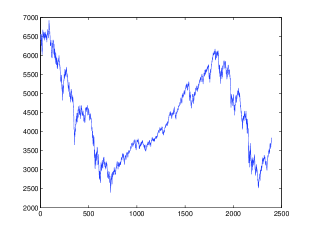
(a) Underlying asset: daily values of the CAC from 28 April 2000 until 18 September 2009

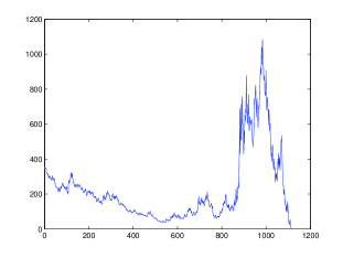
(b) Option: CFU9PY3500 daily prices from 9 May 2009 until 18 September 2009

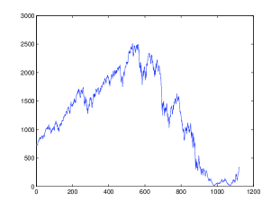
(c) Option: CFU9CY3500 daily prices from 9 May 2009 until 18 September 2009

Figure 1: Daily data

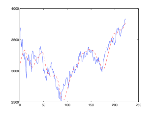
(a) Underlying asset: daily values during the last 223 days, and trend (- -)

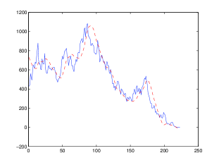
(b) Option: daily values during the last 223 days, and trend (- -)

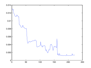
(c) Daily interest rate $r$

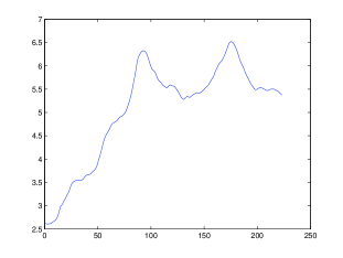
(d) $\Delta$ tracking

Figure 2: Example 1: CFU9PY3500

(a) Underlying asset: values during the last 223 days, and trend (- -)

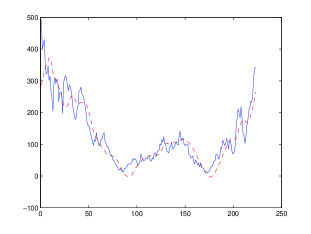
(b) Option: values during the last 223 days, and trend (- -) (- -)

(c) Daily interest rate $r$

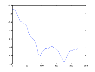
(d) $\Delta$ tracking

Figure 3: Example 2: CFU9CY3500

III-B Abrupt changes

III-B1 Forecasts

We assume that an abrupt change, i.e., a jump, is preceded by “unusual” fluctuations around the trend, and further develop techniques from [16], and from [13, 14]. In Figure 4-(a), which displays forecasts of abrupt changes, the symbols $o$ indicate if the jump is upward or downward.

III-B2 Dynamic hedging

Taking advantage of the above forecasts allows to avoid the risk-free tracking strategy (5), which would imply too strong variations of $\Delta$ and cause some type of market illiquidity. The Figures 4-(b,c,d) show some preliminary attempts, where other less “violent” open-loop tracking controls have been selected.

Remark III.1

Numerous types of dynamic hedging have been suggested in the literature in the presence of jumps (see, e.g., [5, 33, 39] and the references therein). Remember moreover the well known lack of robustness of the BSM setting with jumps [8].

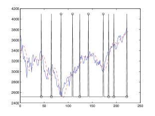
(a) Underlying (–), trend (- -), prediction of abrupt change locations (l) and their directions (o)

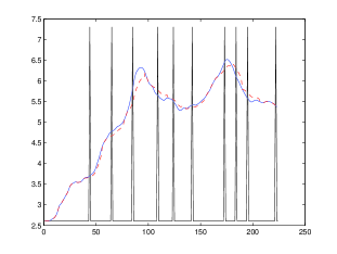
(b) Risk-free $\Delta$ tracking (–) and $\Delta$ tracking (- -), prediction of abrupt change locations (l)

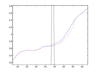
(c) Zoom on (b)

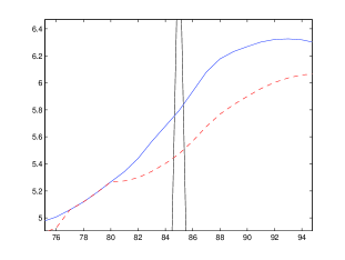
(d) Zoom on (b)

Figure 4: Example 1 (continued): CFU9PY3500

IV Conclusion

Lack of space prevented us from

• examining more involved options, futures, and other derivatives, than in Section II-C,

• thorough numerical and experimental comparisons with the BSM delta hedging.

Subsequent works will do that, and also revisit along the same lines other notions which are related to variances and covariances.

We will

• not try to replace the Gaussian assumptions by more “complex” probabilistic laws,

• further tackle uncertainty by going deeper into the Cartier-Perrin theorem [4], i.e., via a renewed approach of time series.

This is an extreme departure from most today’s criticisms of mathematical finance.

Acknowledgement. The authors would like to thank Frédéric Hatt (Mereor Investment Management and Adivisory, SAS) for stimulating discussions.

References

- [1] Béchu T., Bertrand E., Nebenzahl J., L’analyse technique ( éd.), Economica, 2008.
- [2] Bernhard P., El Farouq N., Thiery S., Robust control approach to option pricing: a representation theorem and fast algorithm, SIAM J. Control Optimiz., 46, 2280–2302, 2007.
- [3] Black F., Scholes M., The pricing of options and corporate liabilities, J. Political Economy, 3, 637–654, 1973.
- [4] Cartier P., Perrin Y., Integration over finite sets, in Nonstandard Analysis in Practice, F. & M. Diener (Eds), Springer, 1995, pp. 195-204.
- [5] Cont R., Tankov P., Financial Modelling with Jump Processes, Chapman & Hall/CRC, 2004.
- [6] Dacorogna M.M., Gençay R., Müller U., Olsen R.B., Pictet O.V, An Introduction to High Frequency Finance. Academic Press, 2001.
- [7] Derman, E., Taleb N., The illusion of dynamic delta replication, Quantitative Finance, 5, 323–326, 2005.
- [8] El Karoui N., Jeanblanc-Picqué M., Shreve S., Robustness of the Black and Scholes formula, Math. Finance, 8, 93–126, 1998.
- [9] Fliess M., Analyse non standard du bruit, C.R. Acad. Sci. Paris Ser. I, 342, 797–802, 2006.
- [10] Fliess M., Join C., Commande sans modèle et commande à modèle restreint, e-STA, 5 (n∘ 4), 1–23, 2008, (available at http//hal.inria.fr/inria-00288107/en/).
- [11] Fliess M., Join C., A mathematical proof of the existence of trends in financial time series, in Systems Theory: Modeling, Analysis and Control, A. El Jai, L. Afifi, E. Zerrik (Eds), Presses Universitaires de Perpignan, 2009, pp. 43–62 (available at http//hal.inria.fr/inria-00352834/en/).
- [12] Fliess M., Join C., Model-free control and intelligent PID controllers: towards a possible trivialization of nonlinear control?, IFAC Symp. System Identif., Saint-Malo, 2009 (available at http//hal.inria.fr/inria-00372325/en/).
- [13] Fliess M., Join C., Towards new technical indicators for trading systems and risk management, IFAC Symp. System Identif., Saint-Malo, 2009 (available at http//hal.inria.fr/inria-00370168/en/).
- [14] Fliess M., Join C., Systematic risk analysis: first steps towards a new definition of beta, COGIS, Paris, 2009 (available at http//hal.inria.fr/inria-00425077/en/).
- [15] Fliess M., Join C., A model-free approach to delta hedging, Technical Report, 2010 (available at http//hal.inria.fr/inria-00457222/en/).
- [16] Fliess M., Join C., Mboup M., Algebraic change-point detection, Applicable Algebra Engin. Communic. Comput., 21, 131–143, 2010.
- [17] Fliess M., Join C., Sira-Ramírez H., Non-linear estimation is easy, Int. J. Model. Identif. Control, 4, 12–27, 2008 (available at http//hal.inria.fr/inria-00158855/en/).
- [18] García Collado F.A., d’Andréa-Novel B., Fliess M., Mounier H., Analyse fréquentielle des dérivateurs algébriques, XXIIe Coll. GRETSI, Dijon, 2009 (available at http//hal.inria.fr/inria-00394972/en/).
- [19] Gençay R., Qi M., Pricing and hedging derivative securities with neural networks: bayesian regularization, early stopping, and bagging, IEEE Trans. Neural Networks, 12, 726–734, 2001.
- [20] Goldstein D.G., Taleb N.N., We don’t quite know what we are talking about when we talk about volatility, J. Portfolio Management, 33, 84–86, 2007.
- [21] Haug E.G., Derivatives: Models on Models, Wiley, 2007.
- [22] Haug E.G., Taleb N.N., Why we have never used the Black-Scholes-Merton option pricing formula, Working paper (5th version), 2009 (available at http//ssrn.com/abstract=1012075).
- [23] Herlin Ph., Fianance : le nouveau paradigme, Eyrolles, 2010.
- [24] Hull J.C., Options, Futures, and Other Derivatives (7th ed.), Prentice Hall, 2007.
- [25] Hutchinson J.M., Lo A.W., Poggio T., A nonparametric approach to pricing and hedging derivative securities via learning networks, J. Finance, 59, 851–889, 1994.
- [26] Join C., Robert G., Fliess M., Vers une commande sans modèle pour aménagements hydroélectriques en cascade, 6e Conf. Internat. Francoph. Automat., Nancy, 2010 (available at http//hal.inria.fr/inria-00460912/en/).
- [27] Jorion P., Financial Risk Manager Handbook (5th ed.), Wiley, 2009.
- [28] Kabbaj T., L’art du trading, Eyrolles, 2008.
- [29] Kirkpatrick C.D., Dahlquist J.R., Technical Analysis: The Complete Resource for Financial Market Technicians (2nd ed.), FT Press, 2010.
- [30] Lobry C., Sari T., Nonstandard analysis and representation of reality, Int. J. Control, 81, 517–534, 2008.
- [31] Mandelbrot N., Hudson R.L., The (Mis)Behavior of Markets: A Fractal View of Risk, Ruin, and Reward, Basic Books, 2004.
- [32] Mboup M., Join C., Fliess M., Numerical differentiation with annihilators in noisy environment, Numer. Algor., 50, 439–467, 2009.
- [33] Merton R., Continuous-Time Finance (rev. ed.), Blackwell, 1992.
- [34] Pham H., Continuous-time Stochastic Control and Optimization with Financial Applications, Springer, 2009.
- [35] Primbs J.A., Dynamic hedging of basket options under proportional transaction costs using receding horizon control, Int. J. Control, 82, 1841–1855, 2009.
- [36] Taleb N., Dynamic Hedging: Managing Vanilla and Exotic Options, Wiley, 1997.
- [37] Taleb N.N., The Black Swan, Random House, 2007.
- [38] Walter C., de Pracontal M., Virus B – Crise financière et mathématique, Seuil, 2009.
- [39] Wilmott P., Derivatives: The Theory and Practice of Financial Enginneering, Wiley, 1998.