Fiber Fabry-Perot cavity with high finesse

Abstract

We have realized a fiber-based Fabry-Perot cavity with CO₂ laser-machined mirrors. It combines very small size, high finesse $\mathcal{F}\geq 130000$, small waist and mode volume, and good mode matching between the fiber and cavity modes. This combination of features is a major advance for cavity quantum electrodynamics (CQED), as shown in recent CQED experiments with Bose-Einstein condensates enabled by this cavity [Y. Colombe et al., Nature 450, 272 (2007)]. It should also be suitable for a wide range of other applications, including coupling to solid-state emitters, gas detection at the single-particle level, fiber-coupled single-photon sources and high-resolution optical filters with large stopband.

1 Introduction

Cavity quantum electrodynamics (CQED) experiments provide insight into the fundamental concepts of quantum mechanics such as entanglement, decoherence and measurement [1, 2]. Additionally, optical CQED is currently growing into a key role in quantum information processing [3], where the transmission of quantum states between distant nodes is a central problem [4], and in entanglement-enhanced metrology [5], where the use of optical cavities has very recently lead to convincing demonstrations of metrologically useful spin squeezing capable of improving the stability of atomic clocks [6]. A fundamental figure of merit of the atom-cavity system is its cooperativity $C$, which up to factors of order 1 is given by

$$C\sim\frac{\sigma_{0}}{\pi w_{0}^{2}}\mathcal{F}\,,$$ (1)

where $\pi w_{0}^{2}$ it the cross-section and $\mathcal{F}$ the finesse of the cavity mode, and $\sigma_{0}$ is the (effective) scattering cross-section of the emitter(s) placed in this mode. For example, the Purcell effect arises when $C>1$ and the efficiency of an important class of single-photon sources scales as $C/C+1$ [7]. In addition to having a high ccoperativity, cavities used in quantum information applications should be miniaturized and fiber-coupled so that they can be used in scalable setups. This motivates considerable efforts to develop miniature high-finesse cavities [8]. However, no cavity type so far unites all desired properties in a single device. Therefore, progress in CQED and its applications hinges on the development of new, miniature cavities with high cooperativity.

Here we describe a fiber-based Fabry-Perot cavity (FFPC) that combines tunability and high finesse with excellent and stable coupling to single-mode optical fibers, which is achieved without mode-matching optics. The waist $w_{0}$ is about an order of magnitude smaller than in the macroscopic high-finesse cavities typically used in optical CQED experiments [1, 2]. The cavity mode is located in free space, making it easy to couple to atomic emitters. The cavity design is based on a new laser machining process where a single, focused CO₂ laser pulse creates a concave depression in the cleaved fiber surface. The first use of this FFPC was in an experiment that demonstrated strong-coupling CQED with Bose-Einstein condensates on atom chips [9], Prompted by these results, the use of such cavities is now being explored with trapped neutral atoms and ions [10, 4], but also with color centers in diamond [11], semiconductors [12, 13] and vibrating sub-wavelength objects [14, 15]. In all of these applications, the small size, ruggedness and built-in fiber coupling of the FFPC are advantageous, favouring its use in hostile environments such as cryostats. Moreover, we have already obtained single-atom cooperativities $C>100$ [9], and still higher values can be expected when using state-of-the art dielectric coatings. This combines with the good fiber coupling, such that decisive progress can be expected from this FFPC for several applications: It should lead to single-photon sources [16] with exceptional overall performance, where not only an atomic excitation is converted into a cavity photon with a probability close to one, but also this photon is efficiently extracted into a single-mode optical fiber. For similar reasons, the FFPC may improve the performance of quantum memories [10, 4], where currently the overall conversion efficiency between the memory qubit and the desired optical mode is still low. It will also enable single-atom state detection (“qubit readout”) with high quantum efficiency, and may enable optical detection with less than a single photon scattered by the emitter [17]. In this article, we present a detailed theoretical and experimental investigation of this new type of fiber cavity.

2 Principle of the fiber Fabry-Perot cavity

The core of our cavity design is a concave, ultralow-roughness mirror surface fabricated directly on the end face of an optical fiber. FFPCs with mirrors on fiber end faces have been built before [18, 19, 20, 21], but until now had only moderate finesse (up to a few 1000), limited by the methods used to fabricate the concave surface on the fiber. Here we use a single CO₂ laser pulse to shape the concave mirror surface, which is then coated with a high-performance dielectric coating. As we show below, this improves the finesse by more than an order of magnitude over the older methods and gives access to an interesting range of small radius of curvature (ROC). As in our earlier design using glued mirrors [19], a stable cavity is then constructed either from one mirror fiber tip facing a macroscopic, planar or concave mirror, or from two closely spaced fiber tips placed face to face (fig. 1). In this article, we will be mainly interested in the second variant.

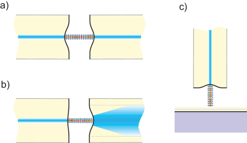
Figure 1: Possible cavity geometries. (a) Cavity made from two single-mode fibers; (b) one single-mode and one multi-mode fiber; (c) single fiber perpendicular to a reflective planar substrate.

Radii of curvature can be fabricated down to $50\,\mu$m and probably below. Because of the small mirror diameter $D$ (smaller than the fiber diameter, which is typically $125\,\mu$m), the mirrors can approach each other very closely (down to a few $\lambda/2$) without touching. The result is a very small mode waist $w_{0}$ between 1 and $2\,\mu$m, and a small mode volume down to a few $\lambda^{3}$. The small $w_{0}$ combined with a length much shorter than the Rayleigh range is the reason for the excellent SM fiber coupling efficiency with no need for mode-matching optics. as we discuss theoretically in sec. 4.4 and demonstrate experimentally in sec. 5.5.

3 Fabrication of concave mirrors on optical fibers

3.1 Laser machining

As will be described in more detail in [22], we have found a parameter regime where a single pulse of CO₂ laser radiation focussed onto the cleaved end face of an optical fiber produces a concave surface with extremely low roughness (figure 2). In this regime, thermal evaporation occurs, while melting is restricted to a thin surface region, avoiding global contraction into a convex shape. This sets it apart from the regimes used in CO₂ laser-based fabrication of microspheres [23] and transformation of microdiscs into high-Q microtoroid resonators [24].

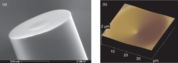
Figure 2: (a) SEM image of a laser-machined fiber end face. (b) AFM measurement of a processed fiber end face with a single pulse of $1.03\,$W and pulse length $40\,$ms, focused to $w_{0}=24\,\mu$m.

We can currently laser machine structures with ROC between $40\,\mu$m and 2 mm, diameters between 10 and $45\,\mu$m, and a surface roughness of about 0.2 nm rms in the optical range. These structures are obtained with CO₂ waist sizes between 18 and $80\,\mu$m, powers in the range $P=0.3\ldots 1.1\,$W and pulse lengths between 5 and 400 ms. A dichroic beam splitter and optical microscope are used to align the fiber with respect to the CO₂ laser focus. In our current setup, we estimate the lateral alignment precision to be better than 2$\,\mu$m.

3.2 Surface analysis

We have laser machined a large number ($>500$) of fiber mirror structures. Initially, we used an AFM to get both profile and roughness data. Scanning the full surface to determine curvatures is a slow process however, so that we could only measure a small number of fibers with this method. To get approximate values for other fibers, we compared them to the well-characterized ones under an optical microscope. More recently, we have used an interferometric microscope for measurements of the large-scale ($>\lambda$) surface topography. This method is fast enough to characterize each individual fiber in reasonable time.

Figure 2 shows SEM and AFM images of representative fiber end faces after the application of a single laser pulse. The section through the center in fig. 3(a) shows a profile which is reasonably well approximated by a gaussian, $z(\rho)=z_{t}\exp(-\rho^{2}/\sigma^{2})$ over a wide parameter range. (A limit is reached for long pulses and big waists, where a rim begins to form around the depression.) Because the profile is not spherical, the local ROC varies with the transverse coordinate (fig. 3(b)). Close to the center of the profile, this variation is slow however, and the shape is well approximated by a circle (fig. 3(c)). We use the central ROC to define the mirror curvature $R$ (fig. 4). The full width at $1/e$ of the gaussian profile gives an estimate of the useful mirror diameter $D$ (cf. 5.4).

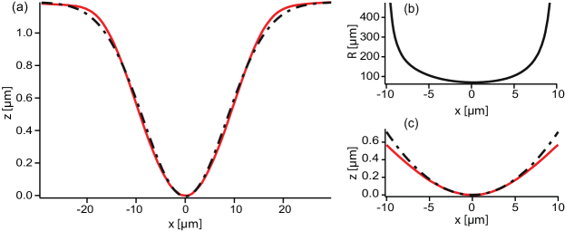
Figure 3: (a) Cut through a profile obtained with the interferometric microscope (red solid line), and its fit by a Gaussian (black dot-dashed line). (b) Local ROC as a function of the transverse coordinate $x$, obtained from a tenth-order polynomial fit to the data in (a) to reduce the effect of measurement noise. (c) Zoom of the data in (a) (red solid line) and a section of a circle with $R=70\,\mu$m (the ROC of the profile at $x=0$) for comparison (black dot-dashed line).

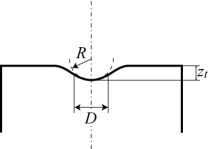
Figure 4: Mirror geometry and parameters. The profile is not spherical; $R$ designates the ROC in the center and $D$ the structure diameter as defined in the text. $z_{t}$ is the depth of the structure.

Because of the approximately gaussian shape of the depression, $R$, $D$ and the total structure depth $z_{t}$ are related by

$$z_{t}\approx\frac{D^{2}}{8R}\,.$$ (2)

For example, a mirror structure with $R=50\,\mu$m and useful diameter $D=10\,\mu$m is only $z_{t}=0.25\,\mu$m deep. With the laser parameters given above, resulting structures are 0.01 to 4 $\mu$m deep and have diameters $D$ between 10 and $45\,\mu$m. ROCs measured at the bottom of the depression are between $40$ and $2000\,\mu$m. Part of the processed surfaces show a slight ellipticity (up to a few percent), which is probably due to an observed astigmatism of the CO₂ beam: when varying the fiber position along the CO₂ beam axis, the beam profile changes from circular to elliptical. Alignment error along this axis translates into ellipticity of the depression. This could easily be improved in a future setup.

AFM measurement areas were between $(500\,\textrm{nm})^{2}$ and $(10\,\mu\textrm{m})^{2}$. To extract surface roughness, we subtract a two-dimensional, fourth-order polynomial that accounts for the concave overall shape and then calculate the isotropic power spectral density (PSD). Integrating the PSD up to $2/\lambda$ consistently yields $\sigma_{\textrm{\small{sc}}}\sim 0.2\pm 0.01\,$nm. (Reference measurements on mica sheets (neglegible roughness) yield $\sigma_{\textrm{noise}}=0.1\,$nm.) A widely used estimate linking this roughness to the scatter loss is [25]

$$\mathcal{S}\approx\left(\frac{4\pi\sigma_{\textrm{\small{sc}}}}{\lambda}\right)^{2}\,.$$ (3)

We thus obtain an estimate of $\mathcal{S}=10\,$ppm for near-infrared light at $\lambda=780\,$nm, assuming a high-quality mirror coating that does not significantly increase this roughness. Such a coating also has very low absorption loss, $\mathcal{A}=2\,$ppm being a realistic value [26]. With a transmission equaling the losses, $\mathcal{T}=\mathcal{S}+\mathcal{A}$, we thus expect a maximum finesse $\mathcal{F}=\pi/(\mathcal{T}+\mathcal{S}+\mathcal{A})\approx 130000$ for a cavity made from two fiber mirrors with identical coatings, and 170000 if the transmission of one mirror is reduced to 2 ppm.

4 Cavity and coupling parameters of FFPCs

4.1 Definitions and optical parameters

We consider cavities consisting of two mirrors, labeled $i=1,2$, of intensity transmission $\mathcal{T}_{i}$, scatter and absorption losses $\mathcal{L}_{i}=\mathcal{S}_{i}+\mathcal{A}_{i}$, and reflectivity $\mathcal{R}_{i}=1-(\mathcal{T}_{i}+\mathcal{L}_{i})$. ROCs are $R_{i}$ and (effective) diameters $D_{i}$. The optical distance between the mirrors is $L$ (which is slightly larger than the geometric distance $L_{\textrm{geom}}$, cf. sec. 4.2). Basic quantities characterizing the cavity are its free spectral range $\textit{FSR}=2\pi c/(2L)$ and the width of the TEM₀₀ cavity resonances, usually expressed as FWHM frequency $\delta\nu$ in laser physics and as HWHM angular frequency

$$\kappa=\frac{2\pi\delta\nu}{2}=\frac{c\mathcal{L}_{\textrm{tot}}}{4L}=\frac{\pi c}{2L\mathcal{F}}$$ (4)

in CQED. Here, $\mathcal{L}_{\textrm{tot}}$ is the round-trip loss ($\mathcal{L}_{\textrm{tot}}=\mathcal{T}_{1}+\mathcal{T}_{2}+\mathcal{L}_{1}+\mathcal{L}_{2}$ if there are no additional losses such as clipping). The cavity finesse is

$$\mathcal{F}=\frac{\textit{FSR}}{2\kappa}=\frac{2\pi}{\mathcal{L}_{\textrm{tot}}}\,.$$ (5)

In contrast to the quality factor $Q=\nu/\delta\nu=\mathcal{F}L/(\lambda/2)$, the finesse depends only on the properties of the mirror coatings and not on the cavity length (as long as the mirror diameters $D_{i}$ are large enough to neglect clipping loss – see below).

4.2 Waist radius

In many applications, the foremost requirement is a small waist $w_{0}$ in order to optimize coupling to an emitter located inside the cavity. In the symmetric case $R_{1}=R_{2}=R$,

$$w_{0}=\sqrt{\frac{\lambda}{2\pi}}\left(L\left(2R-L\right)\right)^{\frac{1}{4}}\,.$$ (6)

(fig. 5, left). With macroscopic supermirrors, the interesting region $w_{0}\lesssim 5\,\mu$m is only accessible in the near-concentric regime $L\sim 2R$, which is difficult or impossible to exploit due to the extreme alignment sensitivity in this regime. Existing macroscopic FP cavities (FPCs) rather have $w_{0}\sim 20\,\mu$m. The FFPC design makes it possible to enter the interesting regime of small $L$ and small $R$ simultaneously, which is inaccessible to macroscopic cavities. Typical $R$ values for our laser-machined fiber mirrors are in the $100\,\mu$m range, two to three orders of magnitude smaller than for traditional high-finesse FPCs. Additionally, for a given $R$, the length of the fiber cavity can be made much smaller than for its macroscopic counterpart, because of the smaller mirror diameter. (The length limit is reached when the mirrors touch [26].) Both factors contribute to enable exceptionally small waists for an open cavity.

The full expression of $w_{0}$ for non-symmetric cavities can be found in textbooks such as [27]. As with symmetric cavities, small waists are obtained for short cavities ($L\ll R_{1},R_{2}$) and close to the stability limits ($L\approx R_{1}+R_{2}$ and $L\approx|R_{1}-R_{2}|$). For short cavities, the full expression simplifies to

$$w_{0}\approx\sqrt{\frac{\lambda}{\pi}}\left(L\frac{R_{1}R_{2}}{R_{1}+R_{2}}\right)^{\frac{1}{4}}\,.$$ (7)

If furthermore $R_{1}$ and $R_{2}$ are substantially different, the minimum waist size is determined by the smaller of the two. For example, if $R_{1}\ll R_{2}$, then

$$w_{0}\approx\sqrt{\frac{\lambda}{\pi}}\left(LR_{1}\right)^{\frac{1}{4}}\,.$$ (8)

This limit particularly applies to half-symmetric cavities ($R_{2}=\infty$). Interestingly, comparison with eq. 6 shows that when replacing one mirror of a short symmetric cavity by a planar one (leaving $L$ unchanged) increases $w_{0}$ by less than $20\,\%$.

To summarize: if we exclude cavities close to the stability limit, then a small-waist cavity should be as short as possible and have at least one strongly curved mirror.

4.3 Minimum length and waist

To determine the smallest possible $w_{0}$ within our fabrication limits, we have to consider how small $L$ can be made. We can currently machine mirror structures with diameters down to $10\,\mu$m. As we have seen in sec. 3.2, the mirror depth is about $z_{t}=250\,$nm for an $R=50\,\mu$m fiber mirror with $D=10\,\mu$m, so that a geometric cavity length as short as $L_{\textrm{geom}}=500\,$nm can be realized even with such a strongly curved mirror. (Note that the $D=10\,\mu$m is still large enough to avoid clipping loss, cf. sec. 4.5.) The part of the field penetrating into the multilayer stack then contributes significantly to the effective cavity length. We account for this effect by setting $L=L_{\textrm{geom}}+\alpha_{\textrm{ml}}\lambda/2$ [26], where the coating materials give $\alpha_{\textrm{ml}}\simeq 1.6$ in our case – dominating over the minimum geometric length. Taking into account this effect and leaving a small gap to introduce atoms, it should still be possible to achieve $L\approx 2\mu$m for all $R$ down to our current fabrication limit $R=50\,\mu$m. A symmetric cavity with $R=50\,\mu$m and $L=5\lambda/2\approx 2.0\,\mu$m then has $w_{0}=1.3\,\mu$m at $\lambda=780\,$nm according to eq. (6). This is more than ten times smaller than the waist of macroscopic CQED cavities and slightly smaller than that of high-Q micropillars [28]. Modeling this mode more accurately would require taking into account light propagation inside the multilayer stack (and not just the stack’s effect on cavity length), and may also require going beyond the paraxial approximation [29].

Minimizing $L$ and $R$ also minimizes the mode volume

$$V_{m}=\frac{\pi}{4}w_{0}^{2}L=\lambda/8\sqrt{2RL^{3}-L^{4}}\,,$$ (9)

where the second form is for the symmetric case. With the parameters above, $V_{m}\approx 2.6\,\mu\mbox{m}^{3}\approx 5.5\lambda^{3}$. $V_{m}$ enters in CQED coupling rates, which will be discussed below in sec. 4.6.

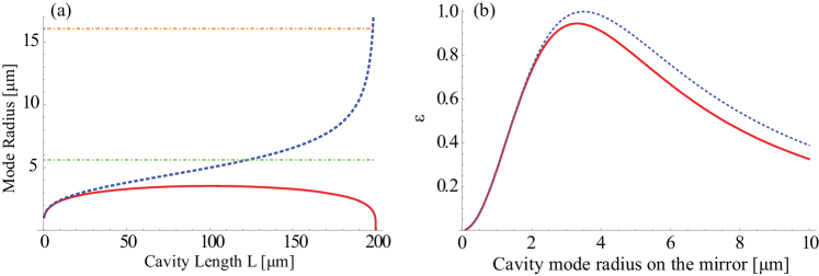
Figure 5: (a) Waist radius $w_{0}$ (red solid line) and mode radius $w_{1,2}$ on the mirrors (blue dashed line) for a cavity with $R_{1}=R_{2}=100\,\mu$m and $\lambda=780\,$nm. Dot-dashed lines indicate the maximum $w_{1,2}$ for a mode-matching efficiency $\epsilon=0.8$ to a fiber with mode field radius $w_{f}=3.5\,\mu$m (green line) and for neglegible clipping loss up to $\mathcal{F}=150000$ assuming mirror diameter $D=45\,\mu$m (orange line). (b) Power coupling efficiency $\epsilon$ between a SM fiber (mode field radius $w_{f}=3.5\,\mu$m) with a mirror of curvature $R=150\,\mu$m and the cavity mode, as a function of the cavity mode radius $w_{m}$ on the mirror. Red, solid line: Full model taking into account wavefront curvature and the lensing effect of the mirror surface (eq. (11)). Blue, dashed line: wavefront curvature and the lensing effect are neglected (10)). The approximation is very good for small $w_{m}$, and remains remarkably accurate even for larger values. The predicted maximum efficiency is $\epsilon=1$ for $w_{m}=3.5\,\mu$m in the approximation and $\epsilon\approx 0.95$ for $w_{m}\approx 3.3\,\mu$m in the full expression.

4.4 Fiber coupling

As the cavity mirrors are part of the incoupling and outcoupling fibers, coupling to and from the cavity is robust and stable over time. This is one key advantage of the FFPC. There are no mode-matching lenses, so coupling efficiency is given directly by the mode matching between the mode leaving the fiber and the cavity mode. If single-mode operation is not required – such as for the output fiber in a cavity transmission measurement – a multimode (MM) fiber can be used on the output side [9]. This virtually eliminates coupling loss and also makes the cavity more robust against various types of misalignment, such as centering errors between the mirror and the fiber core. But even for SM fibers, the coupling efficiency $\epsilon$ is typically very high, in spite of the strong mirror curvature. For example, we have measured $\epsilon>85\%$ for a SM fiber and a mirror with $R=450\,\mu$m (see sec. 5.5).

This high efficiency can be seen as a consequence of the small cavity mode radius, which leads to small phase difference across the relevant mode cross-sections even for strongly curved wavefronts. To get a feeling for the orders of magnitude, consider a spherical wavefront with ROC $R\gg\lambda$. This wavefront deviates from its tangential plane by $\lambda/2$ when the transverse coordinate $\rho$ reaches $\rho_{\lambda/2}\lambda\approx\sqrt{R/\lambda}$, so even on an $R=100\,\mu$m mirror and $\lambda=1\,\mu$m, the mode radius can be as large as $10\,\mu$m before it deviates from planar by $\lambda/2$. Typical mode field radii in SM fibers are much smaller than this. This has several simplifying consequences: First, the lensing effect by the curved fiber surface can be neglected, and second, the power coupling efficiency $\epsilon$ between the fiber and cavity modes can be approximated simply by the overlap integral of the fiber and cavity mode intensity distributions, neglecting phase mismatch. For a SM fiber with its nearly gaussian transverse mode profile of radius $w_{f}$, and assuming that the cavity mode is well aligned with the fiber axis, we thus obtain the simple estimate

$$\epsilon\approx\left(\frac{2w_{f}w_{m}}{w_{f}^{2}+w_{m}^{2}}\right)^{2}\,,$$ (10)

where $w_{m}$ is the cavity mode’s radius on the mirror. A more complete expression including lensing effect and wavefront curvature is

$$\epsilon=\frac{4}{\left(\frac{w_{f}}{w_{m}}+\frac{w_{m}}{w_{f}}\right)^{2}+\left(\frac{\pi n_{f}w_{f}w_{m}}{\lambda R}\right)^{2}}\,,$$ (11)

where $n_{f}$ is the refractive index of the fiber and $R$ the ROC of the mirror. This expression is derived in the appendix. What it still ignores is misalignment between the mirror and the fiber axis.

In figure 5(right), $\epsilon$ is plotted as a function of $w_{m}$. Optimum coupling occurs around $w_{m}=w_{f}$. The remaining mismatch is due to mirror curvature. To minimize it, $R$ should be chosen as large as possible. $\epsilon=1$ is achieved on the planar side ($R=\infty$) of a half-symmetric cavity where $L$ and the curvature of the second mirror are chosen such that $w_{m}=w_{f}$. A possible drawback of this configuration is its waist size, $w_{0}=w_{f}$: $w_{f}$ is typically much larger than the minimum $w_{0}$ which FFPCs can achieve.

If a MM fiber is used on the outcoupling side, the coupling coefficient is determined by its numerical aperture $NA=\sin\Theta_{\textrm{acc}}$. $\Theta_{\textrm{acc}}$ is the acceptance angle of the fiber, which must be compared to the full divergence angle of the cavity mode. The latter grows from 0 (in the waist) up to $2\lambda/(\pi w_{0})$ (for $z\gg z_{R}$). As an example, for a typical $NA=0.1$ at $\lambda=780\,$nm, in the worst case of a long cavity ($L\gg z_{R}$), the waist can still be made as small as $w_{0}=2.4\,\mu$m before the mode divergence becomes larger than the acceptance angle of the fiber. The large acceptance angle also makes the cavity more robust with respect to misalignment.

4.5 Maximum length and clipping loss

In some applications, a larger mirror distance is required, for example to introduce an object such as a membrane [30]), to minimize trap distortion and heating in an ion trap, or to reduce the FSR. As $L$ is increased, the mode radius on at least one of the mirrors will also increase, and this limits the cavity length through two effects: first, fiber coupling efficiency decreases, which may or may not be a problem depending on the application. Then, cavity finesse decreases due to clipping loss.

In this section, we will consider these effects for just one of the fiber mirrors, calling $D$ the mirror diameter, $w_{m}$ the cavity mode radius on this mirror, and $w_{f}$ the mode field radius in its fiber. We will first determine the maximum allowable $w_{m}$ as imposed by (a) fiber coupling and (b) clipping. The maximum $L$ for a given $w_{m}$ then follows from the standard FPC formulas (c).

(a) Calling $\epsilon_{\min}$ the target fiber coupling efficiency, and using the approximation of eq. (10), $w_{m}$ must fulfill

$$w_{m}\leq w_{\epsilon}:=w_{f}\left(\frac{1}{\sqrt{\epsilon_{\min}}}+\sqrt{\frac{1-\epsilon_{\min}}{\epsilon_{\min}}}\right)\,.$$ (12)

For example, if the fiber coupling efficiency is to be at least $\epsilon_{\min}=0.8$, the cavity mode radius must not be larger than $1.6\,w_{f}$. For the SM fibers used in our cavities ($w_{f}=3.5\,\mu$m), this estimate yields $w_{\epsilon}=5.6\,\mu$m.

(b) To estimate clipping loss on the the finite-diameter fiber mirrors, we conservatively assume a gaussian cavity mode and consider its “spillover” loss upon reflection on a finite-diameter mirror. For a single reflection,

$$\mathcal{L}_{\textrm{cl}}=e^{-2(D/2)^{2}/w_{m}^{2}}\,,$$ (13)

where $w_{m}$ is the mode radius of the mode impinging on the mirror of diameter $D$. If $\mathcal{L}_{\textrm{cl}}$ is to contribute less than 10% to the total loss,

$$\mathcal{L}_{\textrm{cl}}<\frac{\mathcal{L}_{\textrm{tot}}}{10}=\frac{2\pi}{10\mathcal{F}}\,,$$ (14)

the mode radius on the mirror must verify

$$w_{m}\leq w_{\textrm{cl}}:=\alpha_{\textrm{cl}}\frac{D}{2}\qquad\textrm{with}\qquad\alpha_{\textrm{cl}}=\sqrt{\frac{2}{-\ln\left(\frac{2\pi}{10\mathcal{F}}\right)}}\,,$$ (15)

In the finesse range of interest here, $\alpha_{\textrm{cl}}^{-1}\approx 2.2-2.5$. With our current fabrication limit of $D\leq 45\,\mu$m, we thus have $w_{\textrm{cl}}\approx 18\,\mu$m in the most demanding case ($\mathcal{F}\approx 130000$). This limitation is generally less restrictive than the one imposed by good fiber coupling.

(c) Now let us calculate the maximum $L$ by requiring that the actual $w_{m}$ be smaller than these maximum values. From the elementary FPC formulas, we have for a symmetric cavity

$$w_{m}^{2}=w_{0}^{2}\left(1+\left(\frac{\lambda L}{2\pi w_{0}^{2}}\right)^{2}\right)=\frac{L\lambda}{\pi}\sqrt{\frac{1}{1-\left(1-\frac{L}{R}\right)^{2}}}\,.$$ (16)

For a given pair of identical mirrors, the maximum length is

$$L_{\max}=2R\frac{1}{1+\left(\frac{\lambda R}{\pi w_{\max}^{2}}\right)^{2}},$$ (17)

with $w_{\max}=w_{\textrm{cl}}$ or $w_{\epsilon}$ depending on the case. Obviously, if $w_{\max}^{2}\lesssim\lambda R$, this becomes much shorter than the stability limit.

If the application also imposes $w_{0}$, the length limit follows from the first expression in eq. (16):

$$L_{\max}=\frac{2\pi}{\lambda}w_{0}\sqrt{w_{\max}^{2}-w_{0}^{2}}\,.$$ (18)

For example, with $w_{\max}=16\,\mu$m (low clipping loss) and $\lambda=780\,$nm, we find that a cavity with $w_{0}=2\,\mu$m can be made up to $L_{\max}=125\,\mu$m long. The curvature of the cavity mirrors is then $R=67\,\mu$m. Requiring instead $w_{\max}=5.6\,\mu$m (good mode matching) leads to $L_{\max}=84\,\mu$m and $R=48\,\mu$m.

If there are no restrictions on the mode waist, as might be the case for a filter cavity or a membrane cooling experiment for example, $R$ can be optimized to further increase $L$ while keeping $w_{1,2}$ small (right expression in eq. (16)). The length limit for the symmetric cavity case then becomes

$$L_{\max}=\frac{\pi}{\lambda}w_{\max}^{2}$$ (19)

and is attained for a confocal cavity ($R=L$). In other words, for a given, long $L$, the confocal configuration has the smallest mode radii on the mirrors, and therefore optimizes both mode matching and finesse. Taking again $\lambda=780\,$nm and $w_{\max}=16\,\mu$m (low clipping loss), we find $L_{\max}=1\,$mm, which is of the same order as the limit imposed by the stability criterion for our maximum ROC. Thus, within this simple model, clipping loss in confocal cavities remains neglegible except for very long wavelength and the confocal cavity length is limited to $L\lesssim 500\ldots 1000\,\mu$m by the attainable ROC. Note however that our simple model does not include other imperfections, such as misalignment between the fiber axis and the center of the mirror. In any case, it should be possible to make still longer cavities from one fiber mirror and one macroscopic mirror with larger diameter and ROC.

The more restrictive requirement $w_{\max}=5.6\,\mu$m (good mode matching) leads to $L_{\max}=126\,\mu$m. This is the longest cavity that can be made if the power transmission between fiber and cavity modes is to be at least $\epsilon_{\min}=0.8$. For comparison, the $L=500\,\mu$m confocal cavity has $\epsilon_{\min}=0.32$, which is still an acceptable value in many cases. For $R_{1}\neq R_{2}$, $w_{i}$ still generally grows with $L$ except in the regions near $L=R_{1}$ and $L=R_{2}$, where the resonator becomes unstable.

4.6 CQED parameters as functions of the cavity parameters

In cavity QED problems, the cavity parameters enter in the form of the coherent single-photon coupling rate $g$ and the incoherent cavity decay rate $\kappa$. It is instructive to consider these rates as functions of $w_{0}$ and $L$ (choice of a gaussian mode), and alternatively as functions of $R$ and $L$ (choice of a pair of mirrors), where we restrict ourselves to the symmetric case for simplicity.

For a cavity mode with frequency $\omega$ and an atom or other emitter (dipole matrix element $\mu$) located at maximum field intensity, the coherent coupling rate is

$$g_{0}=\sqrt{\frac{\mu^{2}\omega}{2\hbar\epsilon_{M}V_{m}}}=\sqrt{\frac{3\lambda^{2}c\gamma}{4\pi V_{m}}}\,,$$ (20)

where $\gamma$ is the HWHM linewidth of the excited state, $\epsilon_{M}$ is the dielectric constant at the location of the emitter ($\epsilon_{M}=\epsilon_{0}$ for free space). The second form applies to a two-level atom in free space; for simplicity we will use this form from now on. $g_{0}$ depends on the cavity parameters through the mode volume ((eq. 9)). Fig. 6 shows an example.

We have already determined the minimum achievable mode volume, $V_{m}\approx 5.5\lambda^{3}$ for $\lambda=780\,$nm (sec. 4.3). This leads to a maximum coupling rate of $g_{0}=2\pi\times 2.8\,$GHz for Rb atoms, about four times the most optimistic projected limit [26] of macroscopic FPCs. Note that the limit of [26] assumes significant future improvements in polishing technology, while our value is calculated with the surface quality and ROC that have already been fabricated and measured.

Maximizing $g_{0}$ requires minimizing $V_{m}$, so reducing the mirror spacing (and adapting the ROC accordingly) maximizes $g_{0}$ for a given $w_{0}$. However, doing so also increases the cavity decay rate (eq. 4). If the goal is to enter as far as possible into the “strong coupling regime” (i.e., $g_{0}>\kappa,\gamma$, or equivalently, resolved coupled-system resonances), the coupling-to-dissipation ratio $g_{0}/\max(\gamma,\kappa)$ may be used as a figure of merit. If the cavity is short – more precisely, if $L<\pi c/(2\mathcal{F}\gamma)$ –, then $\kappa>\gamma$, so that this ratio is optimized by maximizing $g_{0}/\kappa$. With $\mathcal{F}=10^{5}$ and $\gamma/2\pi=3\,$MHz, $\pi c/(2\mathcal{F}\gamma)=250\,\mu$m, which means that typically $\kappa>\gamma$ over the full stability range. Expressing this ratio as a function of the mode and mirror parameters:

$$\frac{g_{0}}{\kappa}=\frac{2\lambda}{\pi^{2}}\sqrt{\frac{3\gamma}{c}}\,\frac{\mathcal{F}\sqrt{L}}{w_{0}}=\frac{2\sqrt{6}}{\pi^{3/2}}\sqrt{\frac{\gamma\lambda}{c}}\frac{\mathcal{F}\sqrt{L}}{\left(L(2R-L)\right)^{1/4}}\,.$$ (21)

Fig. 6 shows an example. As expected, choosing a small $w_{0}$ improves this ratio. Somewhat surprisingly, the ratio also improves with growing cavity length, despite the growing mode volume. This is because $\kappa$ depends on $L$ more strongly than does $g_{0}$. For long cavities, the ratio is determined by $g_{0}/\gamma$, and decreases again.

By contrast, in a large class of applications which notably contains single-photon sources, a more important figure of merit is the single-atom cooperativity $C_{0}$,

$$C_{0}=\frac{g_{0}^{2}}{2\kappa\gamma}=\frac{3\lambda^{2}}{\pi^{3}}\frac{\mathcal{F}}{w_{0}^{2}}=\frac{6\lambda}{\pi}\frac{\mathcal{F}}{\sqrt{2RL-L^{2}}}\,.$$ (22)

$C_{0}$ determines the Purcell factor; the probability for a spontaneous photon to be emitted into the cavity mode is $C_{0}/(C_{0}+1)$. The inverse of $C_{0}$ is called the critical atom number.

In contrast to $g_{0}$, $C_{0}$ does not depend on the mode volume, but only on the mode waist $w_{0}$. Another way of seeing this is by realizing that $C_{0}$ is effectively the optical density of the emitter, which depends on the ratio of its absorption cross-section to the cross-section of the mode, but is independent of the cavity length (as long as $L$ is larger than the emitter size). The conclusion is that the choice of a particular gaussian mode fixes the value of $C_{0}$, no matter where we decide to place the mirrors that confine this mode. The strong curvature of our fiber mirrors enables very small waist size, we have already seen that $w_{0}=1.3\,\mu$m is a realistic value. Combined with the maximum finesse $\mathcal{F}\approx 130000$ (sec. 3.2), eq. (22) predicts $C_{0}=4560$ for the maximum cooperativity that can be achieved at $\lambda=780\,$nm.

To conclude this section, fig. 6 shows CQED parameters as a function of cavity length $L$, taking into account clipping loss, for the following parameters: $\lambda=780\,\mbox{nm},\gamma/(2\pi)=3\,\mbox{MHz},R_{1}=100\,\mu\mbox{m},R_{2}=450\,\mu\mbox{m},D_{1}=D_{2}=30\,\mu\mbox{m}$ and $\mathcal{L}=\mathcal{T}=12\,$ppm per mirror.

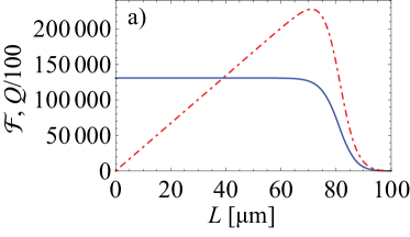
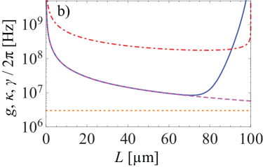
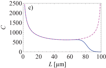
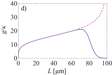
Figure 6: CQED parameters taking into account clipping loss on finite-diameter mirrors, for a cavity with the following parameters: $R_{1}=100\,\mu\mbox{m},R_{2}=450\,\mu\mbox{m},D_{1}=D_{2}=30\,\mu\mbox{m}$, coupling to Rb atoms ($\lambda=780\,\mbox{nm},\gamma/(2\pi)=3\,\mbox{MHz}$). (a) Finesse (blue solid line) and Q factor (red dot-dashed line). The decay for $L\gtrsim 75\,\mu$m is caused by clipping, and is responsible for the increase in $\kappa$ and decrease in $C$ at these lengths. (b) $g_{0}$ without clipping (red, dot-dashed), $\kappa$ without clipping (magenta, dashed) and with clipping loss (solid, blue). Throughout the length range, $\kappa$ is larger than $\gamma$ (orange, dotted). (c) $C$ without clipping (magenta, dashed) and with clipping (blue, solid). Even without clipping loss, the high cooperativity near $L=100\,\mu$m would be difficult to reach in practice, as it occurs at the limit of the stability range. (d) The ratio $g_{0}/\kappa$ without (magenta, dashed) and with clipping (blue, solid). As $\kappa>\gamma$, this ratio quantifies the strong coupling. In contrast to $C_{0}$, it increases for longer cavities as long as clipping is neglegible.

5 Experimental results

We have measured transmission and reflection spectra as well as insertion loss for a variety of FFPCs with mirrors of various curvatures fabricated on SM and MM fibers. All of them had coatings fabricated by Laserzentrum Hannover (LZH) , designed for maximum reflectivity at 780 nm. Note that these are not the best commercially available coatings. We have chosen this supplier as a compromise between coating quality and delay at the time we needed the coatings; the measurements below indicate that still better cavity performance can be achieved by coating the same fibers with “supermirror” coatings, as in [26] for example.

The most comprehensive measurements were done on two cavities, FFP1 and FFP2, which are part of an atom chip experiment in Paris in which we investigate CQED effects with ⁸⁷Rb Bose-Einstein condensates [9] and detection of trapped single atoms. These cavities have been in vacuum for more than 2 years now; periodic remeasurements show no degradation of their performance in spite of their exposition to low-pressure Rb vapor.

While measuring the transmission and reflection spectra is fairly straightforward, other measurments such as insertion loss and mirror losses tend to be more difficult than with macroscopic cavities due to the inherent fiber coupling. In the following subsections we describe our methods and show results for the various parameters.

5.1 Fiber preparation and coating

We have laser-machined a batch of SM and MM gradient index fibers with $125\,\mu$m cladding diameter and $7\,\mu$m mode field diameter / $50\,\mu$m core diameter, respectively. The fibers are metal coated (Cu / Cu alloy), which makes them suitable for ultra-high vacuum use and also shields stray light. Structures with ROC from $90\,\mu$m to $500\,\mu$m and mirror diameters from $20\,\mu$m to $40\,\mu$m were coated in an ion beam sputtering process by LZH. Each fiber was cleaned in aquaeus solution of HCl (H₂O:HCl 5:1) for 2 min in an ultrasonic bath (USB), then rinsed for 2 min (USB) in H₂O and finally for 2 min (USB) in acetone. After cleaning, the surfaces were individually inspected for contaminations and then inserted into a purpose-built holding plate. This procedure was carried out immediately before coating, but outside the cleanroom in which the coating took place.

The dielectric coating has 14 layers of SiO₂ with refractive index $n_{SiO}=1.455$ and 15 layers Ta₂O₅ with $n_{TaO}=2.105$. The calculated transmission of the layer stack is $\mathcal{T}=34\,$ppm at $780\,$nm. Reference substrates with $\sigma\sim 0.1\,$nm rms roughness were coated in the same run.

A microscope inspection of several coated fibers showed that 30-50% of the end faces contained contaminations, some of them making the fibers unemployable. The most likely explanation is that dust remaining on the holding plate contaminated the fibers when they were inserted.

5.2 Coating transmission and losses

To determine the quality of the coatings, we have done various measurements both with reference substrates and with fibers. The LZH carried out a calorimetric absorption loss measurement at 1064nm which yielded $\mathcal{A}=100\pm 30\,$ppm and an Ulbricht sphere total scatter measurement at 633 nm which gave $\mathcal{S}=75\pm 20\,$ppm. Our AFM measurements of the coated reference substrates show a roughness of $\sigma_{sc}=0.20\,$nm rms, an increase of at least 0.1 nm over the value before coating and corresponding to scatter loss $\mathcal{S}=10\,$ppm. Our direct measurement of the transmission of reference substrates yielded $\mathcal{T}=31\pm 5\,$ppm, close to the calculated value. We also built macroscopic cavities from the reference substrates and measured their decay time constant $\tau=\mathcal{F}L/\pi c$ using a fast scan ringdown method [31]. The resulting value $\tau=3.35\,\mu$s obtained for $L=100\,$mm corresponds to a finesse $\mathcal{F}=31000$ and total loss per mirror $\mathcal{T}+\mathcal{L}=\pi/\mathcal{F}=101\,$ppm. Table 1 summarizes these results. The deviations between the different measurement methods suggest isolated defects, possibly the dust particles mentioned above.

Quantity	Method	Macroscopic substrates	Fibers
Absorption loss $\mathcal{A}$	Calorimetric @ 1064 nm	$100\pm 30\,$ppm
	Bistability		$30\pm 6\,$ppm
Scatter loss $\mathcal{S}$	Ulbricht sphere @633 nm	$75\pm 20\,$ppm
	AFM roughness	10 ppm	$23\pm 3\,$ppm
Transmission $\mathcal{T}$	Direct	$31\pm 5\,$ppm
$\mathcal{T}+\mathcal{A}+\mathcal{S}$	Finesse (Fast ringdown)	101 ppm
	Finesse (Cavity scan)		$85\pm 12\,$ppm

Table 1: Summary of mirror loss measurements. Measurements were carried out at 780 nm unless otherwise noted. The finesse measurements, being carried out with two mirrors from the same coating run, provide a fairly accurate value for the total loss per mirror$\mathcal{T}+\mathcal{A}+\mathcal{S}$. The individual measurements of $\mathcal{T}$, $\mathcal{A}$ and $\mathcal{S}$ should add up to the same value within the error margins. This is the case for the fiber mirrors. For the macroscopic substrates however, the sum of the individual measurements is larger than the total value from the finesse measurement. One possible explanation would be low-density defects (dust particles) that increased the loss in the calorimetric and/or Ulbricht sphere measurement.

The total losses for the fiber mirrors were obtained from finesse measurements with short FFPCs, which are discussed in more detail below. Measurements on several cavities yield $\mathcal{F}=37000\pm 5000$, corresponding to total loss $\mathcal{T}+\mathcal{L}=\pi/\mathcal{F}=85\pm 12\,$ppm. Using the value $\mathcal{T}=31\pm 5\,$ppm obtained for the macroscopic substrates, we deduce $\mathcal{L}=(\pi/\mathcal{F})-\mathcal{T}=54\pm 17\,$ppm. An independent estimate of $\mathcal{S}$ comes from the AFM measurements. Like the reference substrates, the coated fibers exhibit an increased surface roughness, in this case to $\sigma_{sc}=0.32\,$nm rms. Using eq. 3, this corresponds to $\mathcal{S}=23\,$ppm. Absorption loss can be estimated from absorption-induced bistability of the cavity (see section 6); we obtained $\mathcal{A}\sim 30$ppm. The sum of these individual estimates is $\mathcal{L}=\mathcal{S}+\mathcal{A}=53\,$ppm. (Considering the errors of the individual measurements, the very good agreement with $(\pi/\mathcal{F})-\mathcal{T}$ is partly fortuitous.)

These measurements consistently indicate that the losses of the FFPCs are dominated by the coatings. In particular, finesse values obtained with macroscopic and fiber mirrors are very similar, in spite of the significantly lower roughness of the macroscopic substrates before coating. The AFM measurements reveal that, indeed, the coatings significantly increased the surface roughness. (For state-of-the art “supermirror” coatings, it is known that this does not occur [26].) There is no indication that the small ROC of the fiber mirrors would cause any significant reduction of the coating quality as compared to the reference substrates. Using state-of-the art coatings should make it possible to fully exploit the surface quality of the laser-machined fibers.

5.3 Fiber cavity mounting and alignment

Fibers were angle-cleaved at their coupling ports and mounted either in a macroscopic mount based on translation stages (“test mount”), or in a dedicated “miniature mount” involving v-grooves and shear piezos on a ceramic baseplate made from Macor (figure 7). The miniature mount has better passive stability, as expected from its low profile and small overall size.

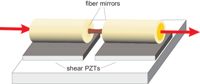
Figure 7: Miniature mount for tunable FFPCs. Piezoelectric transducers (PZTs) are used to scan the cavity length. All other alignment is done during assembly.

In the test mount, fibers are clamped into side-loaded ferrules that are fixed on two micropositioning stages. Together they provide three axes of translation, including fine tunability by integrated piezos, and two angular degrees of freedom. For the miniature mount, we use a similar micropositioning setup to align the fibers during assembly. After glueing, the only adjustable parameter is cavity length within the displacement range of the shear piezos, which is several FSRs. All other alignment is done during assembly, where we apply and cure epoxy glues while monitoring cavity transmission (“active alignment”). We use Epo-Tek 353ND and Epo-Tek 301 to glue the components together. Both are UHV compatible down to $p<10^{-10}\,$mbar. Cavity alignment is observed visually with a stereo microscope (magnification up to 63x) and magnifying video cameras from two axes. After a geometrical preadjustment, the alignment is optimized by maximizing the overall transmission of the fiber cavity, which is scanned over at least one FSR continuously. We did not observe any degradation of the alignment of the glued cavity over time, nor did baking to $100^{\circ}$C leave a measurable irreversible effect once the system had cooled down.

5.4 Tranmission spectrum, finesse and clipping

As a first method to characterize different FFPCs over the whole usable cavity length, we measure transmission spectra at fixed laser frequency, using a piezo actuator to scan $L$ (fig. 8). This can be done with both the test mount and the miniature mount. To obtain a calibration of the length scale, we have used various methods to simultaneously couple several laser frequencies with a well-known difference. To obtain a difference in the GHz range, we use two lasers, typically $\lambda_{1}=780.241\,$nm, locked on the ⁸⁷Rb D2 line, $\lambda_{2}=780.320\,$nm measured with a 6 digit Burleigh wavemeter, $c/\lambda_{1}-c/\lambda_{2}\approx 38.9\,$GHz). With this wavelength calibration, the FSR and the distance $L=c/2\textit{FSR}$ can be determined with an uncertainty below $500\,$nm. To measure the cavity linewidth, a smaller frequency difference is useful, and can be obtained by modulating a single laser at a known frequency in the RF range (fig. 8, left). $\mathcal{F}$ is obtained as the ratio of the FSR and linewidth results.

For a set of three different fiber pairs, we have performed finesse measurements over the whole length range of the cavities (figure 9). All cavities had SM fibers on the input side and MM fibers at the output, and ROC was large on the SM side and small on the MM side: $R_{1}$ between 300 and $400\,\mu$m, $R_{2}$ between 60 and $160\,\mu$m, $D_{1}$ between 20 and $40\,\mu$m, and $D_{2}$ between 30 and $40\,\mu$m. For small mirror distance, we obtain a Finesse of $\mathcal{F}=FSR/\delta\nu=37000\pm 5000$ . The large scatter comes from variation in the alignment quality and from the limited mechanical stability of the test mount. The finesse drops significantly for $L>50\,\mu$m and the resonances vanish in the noise level above $L\sim 70\,\mu$m. This behaviour is well reproduced by including clipping loss (eq. 13) into the calculated finesse: The solid curve in fig. 9 is calculated for $R_{1}=350\,\mu$m, $R_{2}=100\,\mu$m and $D_{2}=23\,\mu$m. Note that the finesse drops sharply over a small distance range. The “cutoff” length at which this occurs depends strongly on the effective mirror diameters. For the cavities in fig. 9, where the waist is located close to mirror 1, it is dominated by $D_{2}$. It will be interesting to repeat such $\mathcal{F}(L)$ measurements for mirrors with different diameters, as this will lead to more accurate predictions of the $D$ values required to reach a desired cavity length.

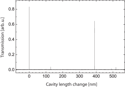
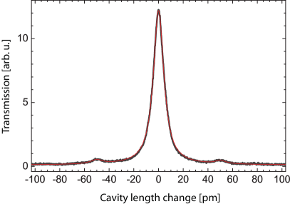
Figure 8: Left: Transmission of the FFP1 cavity at 780 nm. Cavity length is scanned with a piezo actuator, which has been calibrated to obtain an accurate length scale. With optimized alignment, the TEM₀₀ mode is more than 20 times stronger than all higher order modes. Right: Linewidth of the same cavity, measured in transmission. The laser is modulated with sidebands at $\pm 500\,$MHz for frequency calibration. The measurement yields a FWHM linewidth of 100.4 MHz.

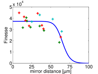
Figure 9: Finesse measurement of three different cavities. For small distance, $\mathcal{F}=37000\pm 5000$. The solid curve is the calculated finesse including clipping loss for $R_{1}=350\,\mu$m, $R_{2}=100\,\mu$m and $D_{2}=23\,\mu$m.

For cavities FFP1 and FFP2, mounted in the miniature mount, we used an improved version of the above protocol. Both lasers were locked to Rb resonances, with a frequency difference of 212 MHz. In this setup, the length could be determined to better than $\lambda/2$ so that the resonance order is exactly known: $d_{1}=99\lambda/2=38.62\,\mu$m, $d_{2}=69\lambda/2=26.9\,\mu$m. With a frequency calibration via amplitude modulation of the laser, we obtain a value for the resonance linewidth of $\delta\nu_{1}=100.4$MHz and $\delta\nu_{2}=156$MHz (fig. 8). Combining these measurements yields $\mathcal{F}_{1}=38600$, $\mathcal{F}_{2}=36000$.

For the FFP1 cavity, we have also measured the dependence on the polarization of the incoming beam. We observe a splitting of $200\,$MHz between two orthogonal, linear input polarizations. Similar birefringence has been observed in macroscopic high-finesse cavities. In our case, it may be related to the ellipticity observed on some of the mirrors.

5.5 Total transmission and mode matching

We have measured transmitted and reflected powers for several cavities in the test and miniature mounts. Our main goal was to obtain information about the coupling efficiency $\epsilon$ between a SM fiber and the cavity. We have investigated this question with cavities having a SM fiber at the input and a MM fiber on the output side. The on-resonance total transmission (from the free-space beam before the first fiber to the beam leaving the second fiber) is

$$\mathcal{T}_{\textrm{tot}}=\epsilon_{2}\left(\frac{\mathcal{T}}{\mathcal{T}+\mathcal{L}}\right)^{2}\epsilon_{1}{\eta_{f}}\,.$$ (23)

The analysis is more complicated than for macroscopic FPCs because neither the coupling efficiency from the free-space beam into the incoupling fiber, ${\eta_{f}}$, nor the mode-matching efficiencies between the fibers and the resonator mode, $\epsilon_{1,2}$, can be determined directly in a non-destructive way. (It would be possible to measure ${\eta_{f}}$ by breaking the fiber.) The measured intensity transmission from before the input of the SM input fiber to after the output of the MM output fiber is 0.094 on resonance for FFP1. (Similar results were obtained for other cavities.) From the mirror transmission measured on the macroscopic substrates, $\mathcal{T}=31\,$ppm, and $\mathcal{T}+\mathcal{L}=\pi/\mathcal{F}=85\,$ppm, the on-resonance transmission of the perfectly mode-matched cavity would be $\left(\mathcal{T}/\mathcal{T}+\mathcal{L}\right)^{2}=0.13$. (Note again that this value is limited by the sub-optimum coatings.) We infer that $\epsilon_{2}\epsilon_{1}{\eta_{f}}=0.094/0.13=0.72$. A lower bound for $\epsilon_{1}$ can be obtained by attributing all this loss to the input mode-matching, so $\epsilon_{1}\geq=0.72$. In reality, ${\eta_{f}}$ is responsible for a significant part of the losses. We have estimated ${\eta_{f}}$ by replacing the cavity input fiber with an “open” fiber (no mirror on the output side) of the same type. In this case, the fiber coupling efficiency is easily measured, and never exceeded ${\eta_{f}}_{1,\max}=0.85$ in our setup. A more realistic value is therefore $\epsilon_{1}\gtrsim 0.72/0.85=0.85$. The theoretical maximum value for perfect alignment (eq. 11) is $\epsilon_{1}=0.979$.

Some additional information can be obtained from a reflection measurement. Let us call $P_{i}$ the power incident on the fiber input port and $P_{r}$ the power that emanates from the same port in the reverse direction (which we can measure using a beam splitter). Off resonance or with the second fiber removed, we have

$$P_{r}=\eta_{r}R{\eta_{f}}P_{i}\approx\eta_{r}{\eta_{f}}P_{i}\,.$$ (24)

Here we assume that all light from the input beam which is not coupled into the fiber is lost and contributes neglegibly to the reflected beam. The parameter $\eta_{r}<1$ takes into account that some of the light reflected back from the mirror is not guided by the fiber because the mirror is not planar and may be misaligned. (Note that in general $\eta_{r}\neq\epsilon_{1}$ because the reflected mode is not identical to the cavity mode.) A measurement of $P_{r}$ yields the product $\eta_{r}{\eta_{f}}$. For FFP1, we obtained $\eta_{r}{\eta_{f}}=0.68$. Measuring ${\eta_{f}}$ with an open fiber gave ${\eta_{f}}\approx 0.85$ in this case, so we obtain $\eta_{r}\approx 0.8$. For various test cavities, we obtained $\eta_{r}=0.7\ldots 0.85$.

On resonance, a symmetric cavity excited by a perfectly mode-matched power $P_{i,0}$ reflects

$$P_{r,0}=P_{i,0}\,R\frac{\mathcal{L}^{2}}{(\mathcal{T}+\mathcal{L})^{2}}\approx P_{i,0}\frac{\mathcal{L}^{2}}{(\mathcal{T}+\mathcal{L})^{2}}\,.$$ (25)

Again, we cannot measure $P_{i,0}$ and $P_{r,0}$ directly. $P_{r}$ has two contributions [26] on resonance: the cavity, which is now excited by the mode-matched power $P_{i,0}=\epsilon{\eta_{f}}P_{i}$, reflects according to eq. 25. The mode-matched part of this reflection, $\epsilon P_{r,0}$, is guided back by the fiber. Second, the non-modematched component of the input light, $(1-\epsilon){\eta_{f}}P_{i}$ is reflected on the mirror and a fraction $\eta_{r}^{\prime}$ of it guided back. Unfortunately, $\eta_{r}^{\prime}\neq\eta_{r}$ because the two constants relate to different incident modes. (We expect $\eta_{r}^{\prime}<\eta_{r}$.) In total, we have

$$P_{r}=P_{i}\left((1-\epsilon)\eta_{r}^{\prime}{\eta_{f}}+\epsilon^{2}{\eta_{f}}\frac{\mathcal{L}^{2}}{(\mathcal{T}+\mathcal{L})^{2}}\right)$$ (26)

Because of the additional unknown constant $\eta_{r}^{\prime}$, this formula is difficult to exploit.

5.6 Mode geometry and cavity QED parameters

Strong coupling between an emitter and a resonant cavity gives rise to a split resonance, displaced by $\pm g$ with respect to the empty cavity resonance, where $g$ is the coherent coupling rate (“vacuum Rabi splitting”). Measuring the resonance frequencies of the coupled system can thus be used to determine $g$. The coupling rate $g_{0}$ in sec. 4.6 is the maximum coupling calculated for a point-like particle localized in an antinode of the cavity field. It is straightforward to extend to the position-dependent coupling $g(\mathbf{r})$. Furthermore, for $N$ independent atoms with a density distribution $\rho(\mathbf{r}))$, one finds:

$$g_{N}=\sqrt{N}\overline{g}_{1}\,,\>\textrm{with}\>\>\overline{g}_{1}^{\,2}=\int\frac{\rho(\mathbf{r})}{N}|g(\mathbf{r})|^{2}d\mathbf{r}\,.$$ (27)

In [9], we have measured $g_{N}$ for Bose-Einstein condensates with variable $N$. The atoms were strongly confined and well localized in the region of maximum coupling of cavity FFP1 described above. $N$ was determined independently by absorption imaging. An estimated uncertainty of about a factor 2 in the $N$ measurement dominates the precision to which we can determine $g_{0}$ from this measurement. $\rho(\mathbf{r})$ depends on $N$ and could in principle be taken into account precisely. However, within the uncertainty imposed by the $N$ measurement, the distribution can be considered point-like for $N\lesssim 1000$. $g_{0}$ can be estimated simply as the prefactor of a $\sqrt{N}$ function fitted to the data for small $N$. This estimate gives $g_{0}\approx 200\,$MHz, in agreement with the calculated value.

6 Optomechanical bistability

When scanning the cavity length using an optical power above a certain threshold, we find strong optical bistability induced by absorption in the mirror: the small fraction of the intracavity power that is absorbed in the mirror coating causes local heating and thermal expansion of the mirror and the fiber. This changes the effective cavity length and therefore the cavity field, leading to bistability. We can observe strongly broadened resonance lines when the cavity is scanned towards increasing length, showing an almost linear increase of transmitted power followed by a rapid drop. This is explained by the expansion of the substrate compensating the length change of the scanning piezo. In the other direction (towards shorter cavity length), we see a narrowed line, corresponding to the cavity being pushed across the resonance by the expansion. Figure 10(a) shows the characteristic lineshape for both scan directions.

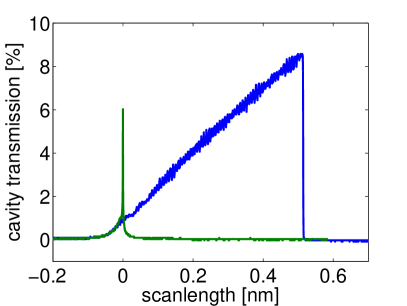
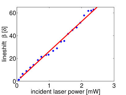
Figure 10: Optical bistability by absorption in the mirrors: (a) Absorption induced thermal expansion leads to two different cavity line shapes when increasing / decreasing the cavity length. Measurement taken with a scan speed $\nu_{\textrm{scan}}=2\times 10^{6}~{}$1/s and $P_{i,0}=2.3~{}$mW. (b) The lineshift $\beta$ as a function of incident power for $\nu_{\textrm{scan}}=2\times 10^{5}~{}$1/s. A linear fit to the data yields $\beta/P_{i,0}=26.3~{}$1/mW.

From the width of the broadened resonances, the absorption in the mirror coatings can be inferred. We measure the total width, as defined in [32], and express it as a multiple $\beta$ of the unperturbed (low-power) linewidth $\kappa$ (i.e., the total width is $\beta\kappa$). In the adiabatic limit, where the temperature distribution in the coating and fiber reaches steady state, $\beta$ is determined by [32]

$$\beta=\frac{8c_{0}C_{\mathrm{ex}}P_{i,0}\mathcal{T}\mathcal{A}\,\mathcal{F}^{3}}{\pi^{3}\lambda k}$$ (28)

with $C_{\mathrm{ex}}$ the effective thermal expansion coefficient of the coating and the fiber, $c_{0}\approx 3.2$ a geometrical factor, $P_{i,0}$ the incident, modematched laser power in the fiber, and $k=1.4\,\textrm{W}\textrm{m}^{-1}\textrm{K}^{-1}$ the thermal conductivity of the fiber. Adiabaticity is met for slow scan velocity $\nu_{\textrm{scan}}<\tau_{r}^{-1}$, where $\nu_{\textrm{scan}}=\dot{\omega}_{\textrm{cav}}/\kappa$ is the scan velocity in units of the cavity linewidth and $\tau_{r}=c_{0}sw_{0}^{2}/k$ the thermal diffusion time with the specific heat per unit volume $s=1.5\times 10^{6}\,\textrm{J}\textrm{m}^{-3}\textrm{K}^{-1}$ for SiO₂. For our parameters, $\tau_{r}=25~{}\mu$s and steady state conditions are expected for $\nu_{\textrm{scan}}<4\times 10^{4}\,\textrm{s}^{-1}$. Due to the limited mechanical stability of the test mount, we had to use a slightly faster scan speed $\nu_{\textrm{scan}}=2\times 10^{5}\,\textrm{s}^{-1}$, so that our measured $\beta$ values are a lower bound to the steady-state value. Fig. 10(b) shows the measured $\beta$ as a function of the incident power. We obtain $\beta/P_{i}=26.3\,$mW^-1. To deduce the mirror absorption from this measurement, the contribution of the coating to the effective thermal expansion coefficient has to be known. From a finite-element simulation, we find that the transient temperature profile extends $\sim 200\,\mu$m into the fiber, and that the mirror coating contributes $\sim 10\%$ to the expansion. Hence $C_{\mathrm{ex}}$ is dominated by the value for SiO₂ $C_{\mathrm{ex,SiO_{2}}}=0.55\times 10^{-6}\,$K^-1 with a $\sim 5\%$ contribution of the Ta₂O₅ layers with $C_{\mathrm{ex,Ta_{2}O_{5}}}=3.6\times 10^{-6}\,$K^-1. With the measured values for the finesse and the mirror transmission, equation (28) yields an absorption loss $\mathcal{A}=35\pm 10\,$ppm, in good agreement with the value obtained in Sec. 5.2. The error for this value stems from the uncertainty of the steady-state value of $\beta$ and of the Ta₂O₅ contribution to the thermal expansion. A more accurate determination could be obtained by measuring the temporal response of the thermal expansion [32]. To avoid the bistability effect, intracavity power should be limited to $P_{i,0}\mathcal{T}/(\mathcal{T}+\mathcal{L})^{2}<3\,\mathrm{W}\times\mathrm{ppm}/\mathcal{A}$.

7 Conclusion

As the results show, FFPCs with laser-machined mirrors combine several desirable properties in a single device. The most important of these are a small mode waist, high finesse, efficient and robust fiber coupling, and open access to the cavity mode. While each of these features individually can also be realized with other cavity types, their combination in a single device is unique to our knowledge, and explains the remarkable interest they are meeting since the publication of [9]. We expect them to be useful in a correspondingly wide range of applications. The devices we have realized so far do not exploit yet the full potential of the laser-machined fiber surface: they are limited by the scatter and absorption losses of sub-optimum mirror coatings. An obvious next step is therefore to have the same fibers coated with “supermirror” [26] coatings, which should enable simultaneous significant increase of finesse and overall transmission. Applications that we are currently investigating in collaboration with specialists from various domains include strong-coupling cavity QED with trapped ions, cavity optomechanics, and coupling to solid-state emitters such as quantum dots and color centers in diamond.

Appendix: Mismatch between fiber and cavity modes

In the following we calculate the coupling efficiency between the mode of a SM fiber and the cavity mode. Both modes are assumed to be gaussian. We take into account the lensing effect due to the concave fiber mirror, and we include the mismatch of wavefront curvatures. What is still neglected in this calculation is the finite coating thickness and any misalignment (centering error) between the mirror and the fiber core.

For concreteness, let us consider light in a SM fiber incident from the left onto the first mirror of an FFPC. The fiber mode is characterized by its mode field radius $w_{f}$. The radius of curvature of the mirror is $R$. We also know the mode radius $w_{m}$ of the cavity mode on this mirror.

The power transmission coefficient between two gaussian modes is [33]

$$\epsilon=\frac{4}{\left(\frac{w_{0}^{\prime}}{w_{0}}+\frac{w_{0}}{w_{0}^{\prime}}\right)^{2}+\frac{s^{2}}{z_{R}z_{R}^{\prime}}}$$ (29)

where $s=z_{0}-z_{0}^{\prime}$ is the distance between the mode waist positions. In our case, the first mode in this formula is the one leaving the fiber through the concave mirror, which has undergone diffraction as the mirror acts like a plano-concave lens. As the mirror is very thin, the mode after passing through the mirror still has the radius $w_{f}$, but has wavefront curvature

$$R_{1}=\frac{R}{n_{f}-1}\,,$$ (30)

where $n_{f}$ is the index of the fiber (we can neglect the very small difference between the core and cladding index).

Knowing its radius and curvature at the mirror position, the first mode is fully determined. The second mode in eq. (29) is the cavity mode, which is fully determined by $R$ and $w_{m}$. Deriving $w_{0}$, $w_{0}^{\prime}$, $z_{R}$ and $z_{R}^{\prime}$ and inserting into eq. (29) gives the final result of eq. 11.

Neglecting the lensing effect of the mirror and the mismatch of wavefront curvature amounts to assuming

$$\left(\frac{\pi n_{f}w_{f}w_{m}}{\lambda R}\right)^{2}\ll\left(\frac{w_{f}}{w_{m}}+\frac{w_{m}}{w_{f}}\right)^{2}\,,$$ (31)

which is a good approximation in many cases, as shown in fig. 5.

References

References

- [1] Haroche S and Raimond J M Exploring the Quantum (Oxford: Oxford University Press, 2006)
- [2] Mabuchi H and Doherty A C 2002 Science 298 1372
- [3] Zoller P e a 2005 Eur. Phys. J. D 36 203
- [4] Kimble H J 2008 Nature 453 1023
- [5] Banaszek K, Demkowicz-Dobrzański R and Walmsley I A 2009 Nature Photonics 3 673
- [6] Leroux I D, Schleier-Smith M H and Vuletić V 2010 Phys. Rev. Lett. 104 073602
- [7] Law C K and Kimble H J 1997 J. Mod. Opt. 44 2067
- [8] Vahala K J 2003 Nature 424 839
- [9] Colombe Y, Steinmetz T, Dubois G, Linke F, Hunger D and Reichel J 2007 Nature 450 272
- [10] Luo L, Hayes D, Manning T, Matsukevich D, Maunz P, Olmschenk S, Sterk J and Monroe C 2009 Fortschr. Phys. 57 1133
- [11] Jelezko F and Wrachtrup J 2006 Phys. Stat. Sol. A 203 3207
- [12] Deveaud B, ed. The Physics of Semiconductor Microcavities (Weinheim: Wiley-VCH, 2006)
- [13] Shields A J 2007 Nature Photonics 1 215
- [14] Jayich A M, Sankey J C, Zwickl B M, Yang C, Thompson J D, Girvin S M, Clerk A A, Marquardt F and Harris J G E 2008 New Journal of Physics 10 095008
- [15] Favero I, Stapfner S, Hunger D, Paulitschke P, Reichel J, Lorenz H, Weig E M and Karrai K 2009 Optics Express 17 12813
- [16] Lounis B and Orrit M 2005 Rep. Prog. Phys. 68 1129
- [17] Poldy R, Buchler B C and Close J D 2008 Phys. Rev. A 78 013640
- [18] D. S M, Nicolas C, Carré A and Carracci S J in Proc. 28th European Conf. on Optical Communication, Copenhagen, Denmark (2002) Paper 10.4.6
- [19] Steinmetz T, Colombe Y, Hunger D, Hänsch T W, Balocchi A, Warburton R J and Reichel J 2006 Appl. Phys. Lett. 89 111110
- [20] Trupke M, Hinds E A, Eriksson S, Curtis E A, Moktadir Z, Kukharenka E and Kraft M 2005 Appl. Phys. Lett. 87 211106
- [21] Muller A, Flagg E B, Metcalfe M, Lawall J and Solomon G S 2009 Appl. Phys. Lett. 95 173101
- [22] Hunger D, Deutsch C, Warburton R and Reichel J 2010 to be published
- [23] Vernooy D W, Furusawa A, Georgiades N P, Ilchenko V S and Kimble H J 1998 Phys. Rev. A 57 R2293
- [24] Armani D K, Kippenberg T J, Spillane S M and Vahala K J 2003 Nature 421 925
- [25] Bennett J M 1992 Meas. Sci. Technol. 3 1119
- [26] Hood C J, Kimble H J and Ye J 2001 Phys. Rev. A 64 033804
- [27] Siegman A E Lasers (Mill Valley: University Science Books, 1986)
- [28] Reitzenstein S, Hofmann C, Gorbunov A, Strauß M, Kwon S H, Schneider C, Löffler A, Höfling S, Kamp M and Forchel A 2007 Appl. Phys. Lett. 90 251109
- [29] van Enk S J and Kimble H J 2001 Phys. Rev. A 63 023809
- [30] Thompson J D, Zwickl B M, Jayich A M, Marquardt F, Girvin S M and Harris J G E 2008 Nature 452 72
- [31] An K, Yang C, Dasari R and Feld M 1995 Opt. Lett. 20 1068
- [32] An K, Sones C, Fang-Yen R, Dasari R and Feld M 1997 Opt. Lett. 22 1433
- [33] Joyce W B and DeLoach B 1984 Appl. Opt. 23 4187