Singular value decomposition applied to compact binary coalescence gravitational-wave signals

Kipp Cannon kipp.cannon@ligo.org LIGO Laboratory, California Institute of Technology, Pasadena, CA 91125, USA    Adrian Chapman LIGO Laboratory, California Institute of Technology, Pasadena, CA 91125, USA    Chad Hanna chad.hanna@ligo.org LIGO Laboratory, California Institute of Technology, Pasadena, CA 91125, USA    Drew Keppel drew.keppel@ligo.org LIGO Laboratory, California Institute of Technology, Pasadena, CA 91125, USA Theoretical Astrophysics, California Institute of Technology, Pasadena, CA 91125, USA    Antony C. Searle antony.searle@ligo.org LIGO Laboratory, California Institute of Technology, Pasadena, CA 91125, USA    Alan J. Weinstein ajw@caltech.edu LIGO Laboratory, California Institute of Technology, Pasadena, CA 91125, USA
Abstract

We investigate the application of the singular value decomposition to compact-binary, gravitational-wave data-analysis. We find that the truncated singular value decomposition reduces the number of filters required to analyze a given region of parameter space of compact binary coalescence waveforms by an order of magnitude with high reconstruction accuracy. We also compute an analytic expression for the expected signal-loss due to the singular value decomposition truncation.

gravitational waves, compact binary coalescence, singular value decomposition

I Introduction

The coalescence of compact binaries composed of neutron stars and or black holes is a promising source of gravitational radiation for ground-based gravitational-wave (GW) detectors. The mass parameters of the GW signal are not known a priori. In order to detect GW from compact binary coalescence (CBC) events, a large number of filter templates are required to to probe the continuous component mass parameter space, (m1,m2)subscript𝑚1subscript𝑚2(m_{1},m_{2}), of possible CBC signals in the detector data to high fidelity Owen (1996); Owen and Sathyaprakash (1999). Template waveforms are distributed in the space such that there is a small maximum loss of signal-to-noise ratio (SNR) (called the “minimal match”) due to the mismatch between an arbitrary point in the mass parameter space and the nearest discrete point of the template bank. A standard choice for the minimal match is 97%, which, for a hexagonally tiled, flat, two-dimensional manifold, corresponds to neighboring templates that have greater than 95% overlap.

This redundancy implies that correlated calculations are required to filter the data with these templates. The singular value decomposition (SVD) can be used to eliminate these correlations by producing orthogonal basis vectors that can be used for filtering and reconstructing the original template bank.

This work will describe how to reduce the computational redundancy in filtering the CBC signal parameter-space in order to more efficiently infer whether or not a GW is present. Specifically, we will explore a purely numerical technique using the SVD to reduce the number of templates required to search the data. We note that others have applied the use of SVD to GW data-analysis to analyze optimal GW burst detection Brady and Ray-Majumder (2004); Heng (2009) and coherent networks of detectors Wen (2008). We also note that significant work has been done to analytically reduce the computational filtering burden using interpolation for certain template waveforms Croce et al. (2000); Mitra et al. (2005).

This paper is organized as follows. First, we describe the framework for CBC filtering in the context of vector inner products. Next we introduce the SVD as a way to reduce the number of filters required to approximately compute those inner products. We then derive an expression for the expected SNR loss in terms of the singular values. Finally, we demonstrate the application of this method to a set of CBC waveforms corresponding to binary neutron star (BNS) coalescences.

II Method

II.1 Matched filtering

CBC searches employ matched filtering as the first step in locating a GW signal Allen et al. (2005). The optimal filtering strategy weights both the detector output and template waveform by the inverse of the amplitude spectral density of the detector noise, a process called “whitening”. Representing both the whitened data and the αthsuperscript𝛼th\alpha^{\mathrm{th}} whitened template waveform as discretely sampled time series, s={si}𝑠subscript𝑠𝑖\vec{s}=\{s_{i}\} and hα={hαi}subscript𝛼subscriptsubscript𝛼𝑖\vec{h}_{\alpha}=\{{h_{\alpha}}_{i}\}, respectively, the output of the matched filter at a specific point in time is given by the vector inner product

ρα=hαs.subscript𝜌𝛼subscriptsuperscript𝛼𝑠\rho_{\alpha}=\vec{h}^{*}_{\alpha}\cdot\vec{s}\,. (1)

In searches for GWs from CBC sources, the signals being sought are chirping sinusoids with an unknown phase. The search over phase is accomplished through the use of complex-valued templates where hαsubscript𝛼\Re\vec{h}_{\alpha} contains the cosine-like phase and hαsubscript𝛼\Im\vec{h}_{\alpha} contains the sine-like phase. The filter output can be maximized over template phase by evaluating |ρα|subscript𝜌𝛼\left\lvert\rho_{\alpha}\right\rvert.

In the absence of a GW signal, the whitened detector data consists only of noise, n={ni}𝑛subscript𝑛𝑖\vec{n}=\{n_{i}\}, and is a stationary, zero-mean, unit-variance, Gaussian random process, so

ni=0,delimited-⟨⟩subscript𝑛𝑖0\displaystyle\langle n_{i}\rangle=0\,, (2a)
ninj=δij,delimited-⟨⟩subscript𝑛𝑖subscript𝑛𝑗subscript𝛿𝑖𝑗\displaystyle\langle n_{i}n_{j}\rangle=\delta_{ij}\,, (2b)

where \langle\,\,\rangle denotes the ensemble average. When the template waveforms are normalized such that hαhα=hαhα=1subscript𝛼subscript𝛼subscript𝛼subscript𝛼1\Re\vec{h}_{\alpha}\cdot\Re\vec{h}_{\alpha}=\Im\vec{h}_{\alpha}\cdot\Im\vec{h}_{\alpha}=1, (2) yields

hαn=0,delimited-⟨⟩subscriptsuperscript𝛼𝑛0\displaystyle\langle\vec{h}^{*}_{\alpha}\cdot\vec{n}\rangle=0\,, (3a)
(hαn)2=(hαn)2=1.delimited-⟨⟩superscriptsubscript𝛼𝑛2delimited-⟨⟩superscriptsubscript𝛼𝑛21\displaystyle\langle(\Re\vec{h}_{\alpha}\cdot\vec{n})^{2}\rangle=\langle(\Im\vec{h}_{\alpha}\cdot\vec{n})^{2}\rangle=1\,. (3b)

When (3) is true, ραsubscript𝜌𝛼\rho_{\alpha} is called the SNR and indicates how likely it is that a signal is present in the data at that point in time Wainstein and Zubakov (1962).

As explained in Sec. I, hαhα>0.95subscript𝛼subscriptsuperscript𝛼0.95\vec{h}_{\alpha}\cdot\vec{h}_{\alpha^{\prime}}>0.95 for adjacent templates. For those templates, ραsubscript𝜌𝛼\rho_{\alpha} and ραsubscript𝜌superscript𝛼\rho_{\alpha^{\prime}} differ by at most 5%. This suggests the existence of an approximation scheme that would allow the SNRs to be computed to reasonable accuracy without explicitly evaluating all the template inner products. Next, we will look at how the truncated SVD can be used to replace the template bank with an approximate, lower-rank, orthogonal basis from which the SNRs can be reconstructed.

II.2 Reducing the number of filters with truncated singular value decomposition

The waveforms are parameterized by their component masses and we denote the αthsuperscript𝛼th\alpha^{\rm th} template waveform of the M𝑀M templates required to search a given parameter space as hα={h(m1,m2,ti)}subscript𝛼subscript𝑚1subscript𝑚2subscript𝑡𝑖\vec{h}_{\alpha}=\{h(m_{1},m_{2},t_{i})\}. Rather than filter the data with N=2M𝑁2𝑀N=2M real-valued filters (M𝑀M complex-valued filters), we linearly combine the output of a basis set of fewer, real-valued, filters, uμsubscript𝑢𝜇\vec{u}_{\mu}, to reproduce ραsubscript𝜌𝛼\rho_{\alpha} to the desired accuracy, ραsubscriptsuperscript𝜌𝛼\rho^{\prime}_{\alpha}. The goal is to have

ρα=μ=1NAαμ(uμs),subscriptsuperscript𝜌𝛼superscriptsubscript𝜇1superscript𝑁subscript𝐴𝛼𝜇subscript𝑢𝜇𝑠\rho^{\prime}_{\alpha}=\sum_{\mu=1}^{N^{\prime}}A_{\alpha\mu}(\vec{u}_{\mu}\cdot\vec{s})\,, (4)

where 𝐀𝐀{\bf A} is the complex-valued reconstruction matrix we wish to find and the number of inner products is reduced from N𝑁N to Nsuperscript𝑁N^{\prime}. In order to find the basis vectors, uμsubscript𝑢𝜇\vec{u}_{\mu}, we use the SVD of the real-valued template matrix, 𝐇𝐇{\bf H}

𝐇={Hμj}={h1,h1,h2,h2,,hM,hM},𝐇subscript𝐻𝜇𝑗subscript1subscript1subscript2subscript2subscript𝑀subscript𝑀{\bf H}=\{H_{\mu j}\}\\ =\{\Re\vec{h}_{1},\Im\vec{h}_{1},\Re\vec{h}_{2},\Im\vec{h}_{2},...,\Re\vec{h}_{M},\Im\vec{h}_{M}\}\,, (5)

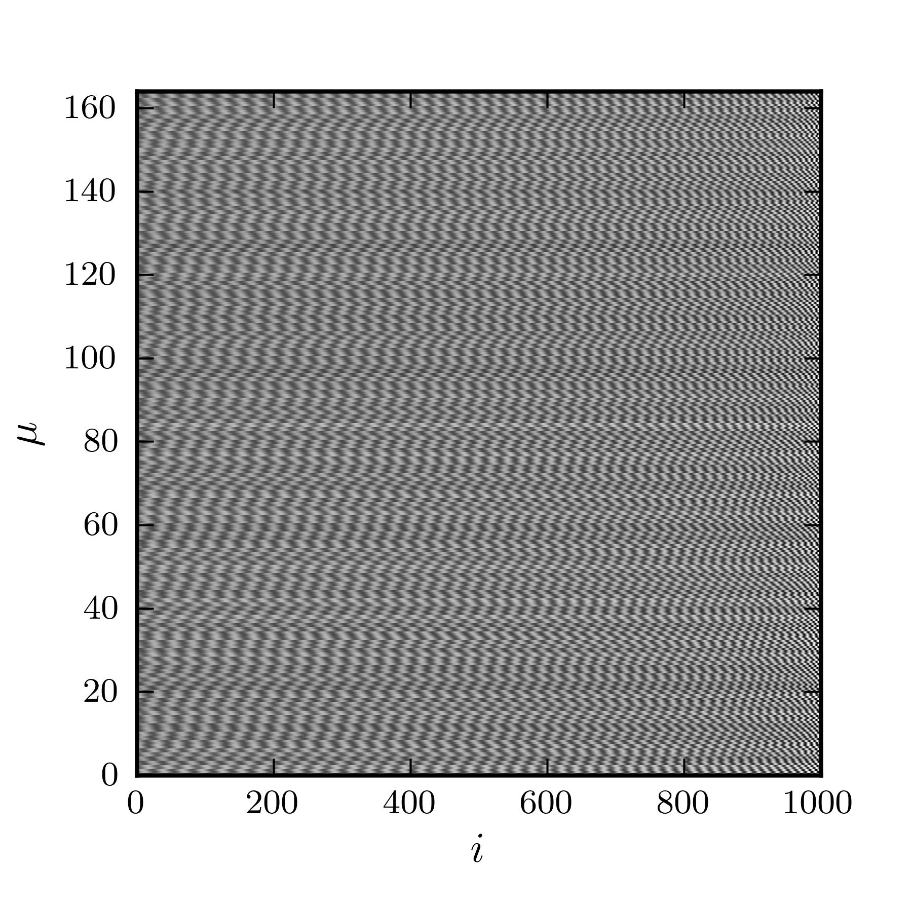
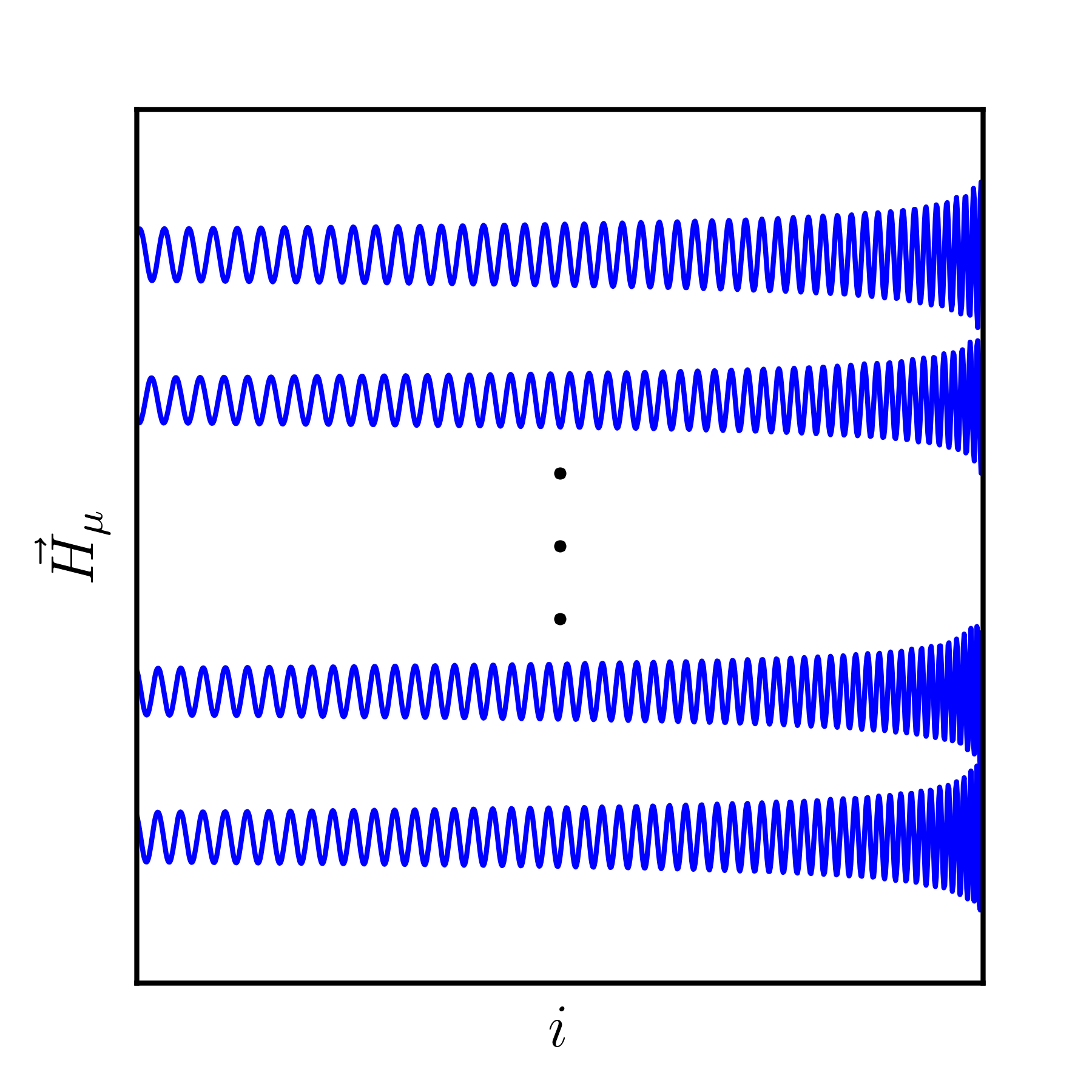
where μ𝜇\mu identifies rows of 𝐇𝐇{\bf H} and indexes the filter number, and j𝑗j identifies the columns of 𝐇𝐇{\bf H} and indexes sample points. In this definition, the row vectors H(2α1)subscript𝐻2𝛼1\vec{H}_{(2\alpha-1)} and H(2α)subscript𝐻2𝛼\vec{H}_{(2\alpha)} are, respectively, the real and imaginary parts of the αthsuperscript𝛼th\alpha^{\rm th} complex waveform, hαsubscript𝛼\vec{h}_{\alpha}. An illustrative template matrix can be seen in Fig. 1.
Refer to caption
Refer to caption
Figure 1: An example template matrix, 𝐇𝐇{\bf H}. Top: An illustration of how the input template time series is packed into the template matrix. Bottom: The matrix of the template time series where the y-axis indicates the template waveform and the x-axis indicates the time samples. It should be noted that these waveforms have been shortened and have not been whitened for illustrative purposes.

The SVD factors a matrix such that (Galassi et al., 2009, Sec. 14.4)

Hμj=ν=1Nvμνσνuνj,subscript𝐻𝜇𝑗superscriptsubscript𝜈1𝑁subscript𝑣𝜇𝜈subscript𝜎𝜈subscript𝑢𝜈𝑗H_{\mu j}=\sum\limits_{\nu=1}^{N}v_{\mu\nu}\sigma_{\nu}u_{\nu j}\,, (6)

where 𝐯𝐯{\bf v} is an orthonormal matrix of reconstruction coefficients whose columns, vμνsubscript𝑣𝜇𝜈v_{\mu\nu}, satisfy

μvμνvμλ=δνλ,subscript𝜇subscript𝑣𝜇𝜈subscript𝑣𝜇𝜆subscript𝛿𝜈𝜆\sum_{\mu}v_{\mu\nu}v_{\mu\lambda}=\delta_{\nu\lambda}\,, (7)

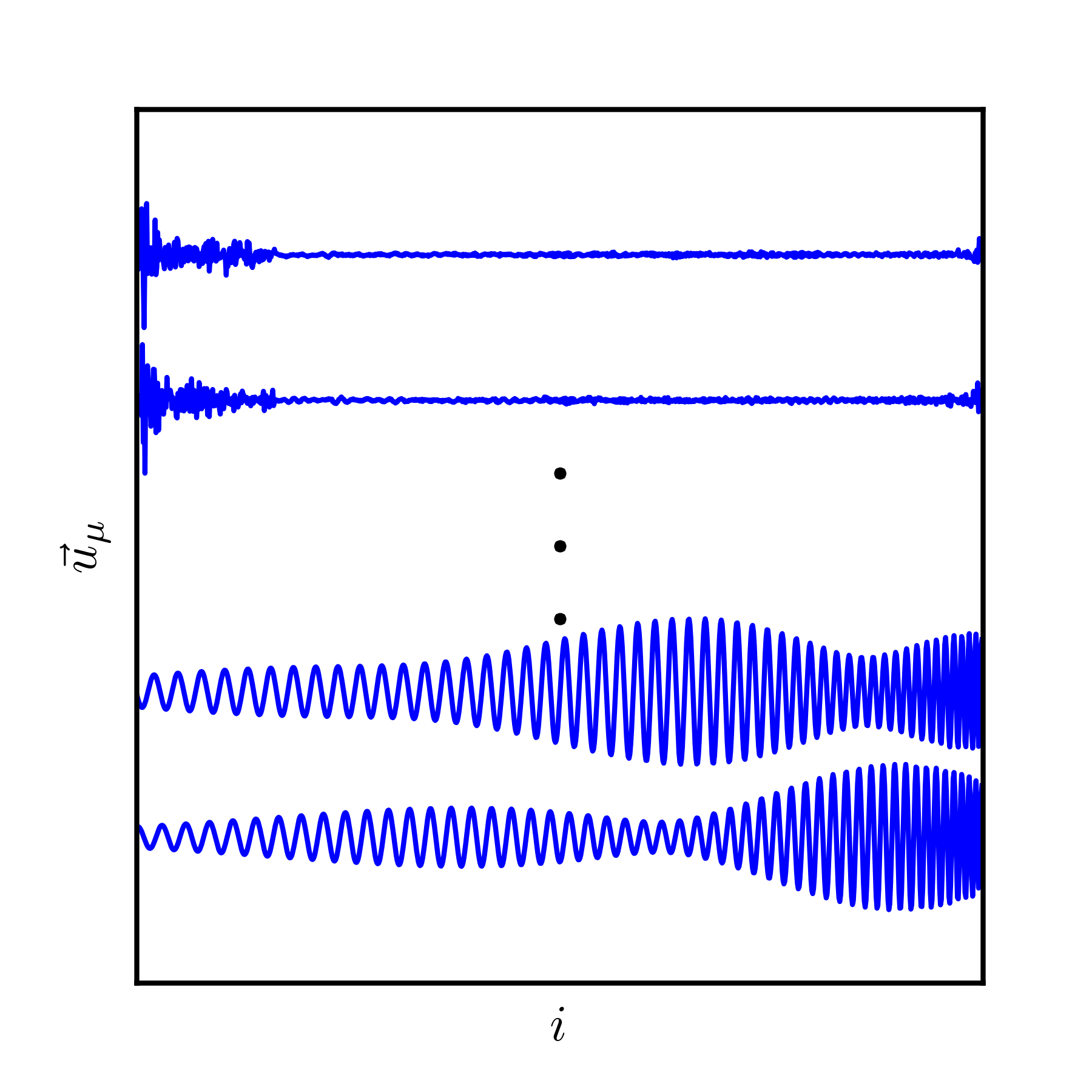
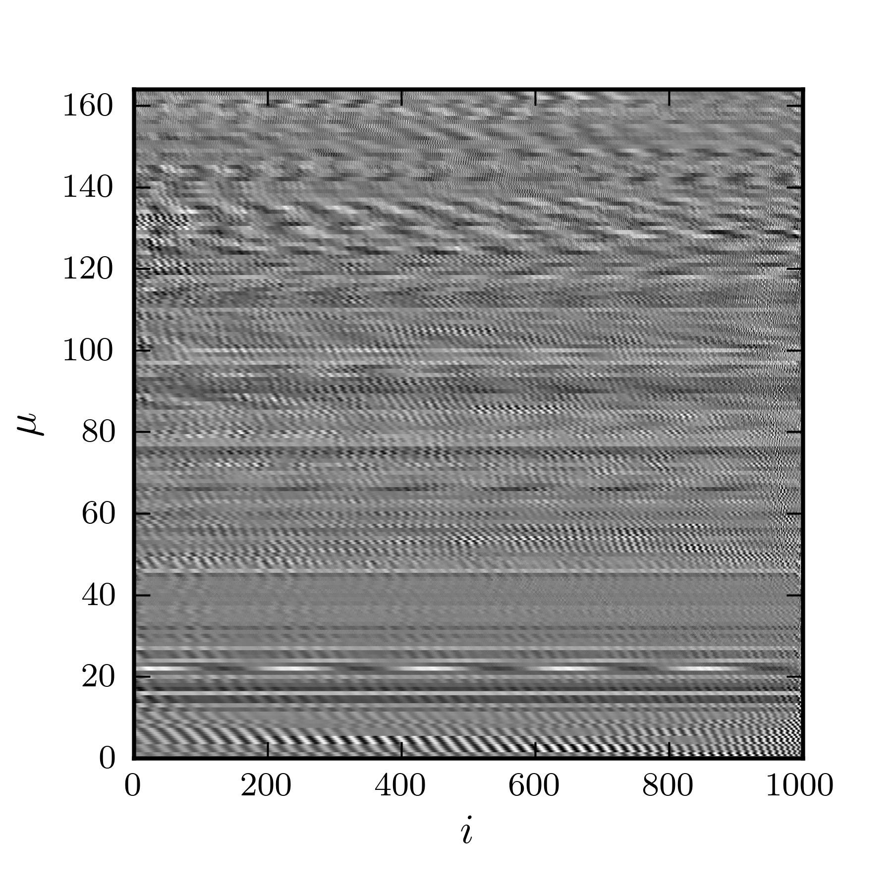
σ𝜎\vec{\sigma} is a vector of singular values ranked in order of importance in reconstructing the 𝐇𝐇{\bf H}, and 𝐮𝐮{\bf u} is a matrix of orthonormal bases (e.g. an illustration can be found in Fig. 2) whose rows are basis vectors, uμsubscript𝑢𝜇\vec{u}_{\mu}, satisfying

juμjuνj=δμν.subscript𝑗subscript𝑢𝜇𝑗subscript𝑢𝜈𝑗subscript𝛿𝜇𝜈\sum_{j}u_{\mu j}u_{\nu j}=\delta_{\mu\nu}\,. (8)
Refer to caption
Refer to caption
Figure 2: An example basis matrix, 𝐮𝐮{\bf u}. Top: An illustration of the resulting orthonormal basis vectors ordered from most to least important (bottom to top) in reconstructing 𝐇𝐇{\bf H}. Bottom: The matrix of basis waveforms produced by the SVD. The y-axis indexes the basis waveforms and the x-axis indicates time samples. It should be noted that these basis vectors have been computed from shortened, non-whitened template waveforms as mentioned in Fig. 1 purely for illustrative purposes.

However, since a search for CBC signals only needs waveform accuracies of a few percent to be successful, it is possible to make an approximate reconstruction of 𝐇𝐇{\bf H}

HμjHμj:=ν=1Nvμνσνuνj,subscript𝐻𝜇𝑗subscriptsuperscript𝐻𝜇𝑗assignsuperscriptsubscript𝜈1superscript𝑁subscript𝑣𝜇𝜈subscript𝜎𝜈subscript𝑢𝜈𝑗H_{\mu j}\approx H^{\prime}_{\mu j}:=\sum_{\nu=1}^{N^{\prime}}v_{\mu\nu}\sigma_{\nu}u_{\nu j}\,, (9)

where N<Nsuperscript𝑁𝑁N^{\prime}<N. This reduces the number of rows of 𝐮𝐮{\bf u} used in the reconstruction. We create a new basis matrix 𝐮={uνj}={u1,u2,uN}𝐮subscript𝑢𝜈𝑗subscript𝑢1subscript𝑢2subscript𝑢superscript𝑁{\bf u}=\{u_{\nu j}\}=\{\vec{u}_{1},\vec{u}_{2},...\vec{u}_{N^{\prime}}\}, where ν𝜈\nu indexes the filter number, j𝑗j indexes sample points, and we have discarded the basis vectors that look least like the template waveforms (i.e. with the lowest singular values). We can write (4) as

ραsubscriptsuperscript𝜌𝛼\displaystyle\rho^{\prime}_{\alpha} =(H(2α1)iH(2α))sabsentsubscriptsuperscript𝐻2𝛼1isubscriptsuperscript𝐻2𝛼𝑠\displaystyle=\left(\vec{H}^{\prime}_{(2\alpha-1)}-\mathrm{i}\vec{H}^{\prime}_{(2\alpha)}\right)\cdot\vec{s}
=ν=1N(v(2α1)νσνiv(2α)νσν)(uνs),absentsuperscriptsubscript𝜈1superscript𝑁subscript𝑣2𝛼1𝜈subscript𝜎𝜈isubscript𝑣2𝛼𝜈subscript𝜎𝜈subscript𝑢𝜈𝑠\displaystyle=\sum_{\nu=1}^{N^{\prime}}\left(v_{(2\alpha-1)\nu}\sigma_{\nu}-\mathrm{i}v_{(2\alpha)\nu}\sigma_{\nu}\right)\left(\vec{u}_{\nu}\cdot\vec{s}\right)\,, (10)

where we have made use of the packing of 𝐇𝐇{\bf H} (5) and (9).

II.3 Reconstruction accuracy

As we are not reconstructing the original template waveforms exactly, there will be some inherent mismatch between Hμsubscriptsuperscript𝐻𝜇\vec{H}^{\prime}_{\mu} and Hμsubscript𝐻𝜇\vec{H}_{\mu}. We want to know the expected fractional SNR we will lose because of this difference.

As stated previously, the inner product of a (normalized) template waveform, Hμsubscript𝐻𝜇\vec{H}_{\mu}, with itself is

HμHμ=1=ν=1Nvμν2σν2,subscript𝐻𝜇subscript𝐻𝜇1superscriptsubscript𝜈1𝑁superscriptsubscript𝑣𝜇𝜈2superscriptsubscript𝜎𝜈2\vec{H}_{\mu}\cdot\vec{H}_{\mu}=1=\sum_{\nu=1}^{N}v_{\mu\nu}^{2}\sigma_{\nu}^{2}\,, (11)

where, in the second line, we have made use of the orthogonality of basis vectors (8). A similar relation can be found for the inner product of the reconstructed waveform, Hμsubscriptsuperscript𝐻𝜇\vec{H}^{\prime}_{\mu}, with itself

HμHμ=ν=1Nvμν2σν2=1ν=N+1Nvμν2σν2.subscriptsuperscript𝐻𝜇subscriptsuperscript𝐻𝜇superscriptsubscript𝜈1superscript𝑁superscriptsubscript𝑣𝜇𝜈2superscriptsubscript𝜎𝜈21superscriptsubscript𝜈superscript𝑁1𝑁superscriptsubscript𝑣𝜇𝜈2superscriptsubscript𝜎𝜈2\vec{H}^{\prime}_{\mu}\cdot\vec{H}^{\prime}_{\mu}=\sum_{\nu=1}^{N^{\prime}}v_{\mu\nu}^{2}\sigma_{\nu}^{2}=1-\sum_{\nu=N^{\prime}+1}^{N}v_{\mu\nu}^{2}\sigma_{\nu}^{2}\,. (12)

Because of the orthogonality of the basis vectors (8), the inner product between a template waveform, Hμsubscript𝐻𝜇\vec{H}_{\mu}, with a reconstructed waveform, Hνsubscriptsuperscript𝐻𝜈\vec{H}^{\prime}_{\nu}, is

HμHν=HμHν=HμHν.subscript𝐻𝜇subscriptsuperscript𝐻𝜈subscriptsuperscript𝐻𝜇subscript𝐻𝜈subscriptsuperscript𝐻𝜇subscriptsuperscript𝐻𝜈\vec{H}_{\mu}\cdot\vec{H}^{\prime}_{\nu}=\vec{H}^{\prime}_{\mu}\cdot\vec{H}_{\nu}=\vec{H}^{\prime}_{\mu}\cdot\vec{H}^{\prime}_{\nu}\,. (13)

In addition, the two phases of the templates, which are packed adjacently in 𝐇𝐇{\bf H} (5), are orthogonal

H(2μ1)H(2μ)=ν=1Nv(2μ1)νv(2μ)νσν2=0.subscript𝐻2𝜇1subscript𝐻2𝜇superscriptsubscript𝜈1𝑁subscript𝑣2𝜇1𝜈subscript𝑣2𝜇𝜈superscriptsubscript𝜎𝜈20\vec{H}_{(2\mu-1)}\cdot\vec{H}_{(2\mu)}=\sum_{\nu=1}^{N}v_{(2\mu-1)\nu}v_{(2\mu)\nu}\sigma_{\nu}^{2}=0\,. (14)

This implies that the inner product of the two phases of the approximate waveforms are given as

H(2μ1)H(2μ)subscriptsuperscript𝐻2𝜇1subscriptsuperscript𝐻2𝜇\displaystyle\vec{H}^{\prime}_{(2\mu-1)}\cdot\vec{H}^{\prime}_{(2\mu)} =ν=1Nv(2μ1)νv(2μ)νσν2absentsuperscriptsubscript𝜈1superscript𝑁subscript𝑣2𝜇1𝜈subscript𝑣2𝜇𝜈superscriptsubscript𝜎𝜈2\displaystyle=\sum_{\nu=1}^{N^{\prime}}v_{(2\mu-1)\nu}v_{(2\mu)\nu}\sigma_{\nu}^{2}
=ν=N+1Nv(2μ1)νv(2μ)νσν2.absentsuperscriptsubscript𝜈superscript𝑁1𝑁subscript𝑣2𝜇1𝜈subscript𝑣2𝜇𝜈superscriptsubscript𝜎𝜈2\displaystyle=-\sum_{\nu=N^{\prime}+1}^{N}v_{(2\mu-1)\nu}v_{(2\mu)\nu}\sigma_{\nu}^{2}\,. (15)

The average fractional SNR loss, δρα/ρα𝛿subscript𝜌𝛼subscript𝜌𝛼\delta\rho_{\alpha}/\rho_{\alpha}, between a template waveform and the two phases of the same reconstructed waveform is given by

δραρα:=1|ρα||ρα|.assign𝛿subscript𝜌𝛼subscript𝜌𝛼1subscriptsuperscript𝜌𝛼subscript𝜌𝛼\frac{\delta\rho_{\alpha}}{\rho_{\alpha}}:=1-\frac{\left\lvert\rho^{\prime}_{\alpha}\right\rvert}{\left\lvert\rho_{\alpha}\right\rvert}\,. (16)

The following derives the mismatch in terms the of components we truncate from the SVD. First we compute these terms for a given signal waveform, s=(Aeiϕhα)𝑠𝐴superscripteiitalic-ϕsubscript𝛼\vec{s}=\Re\left(A\mathrm{e}^{\mathrm{i}\phi}\vec{h}_{\alpha}\right), with phase, ϕitalic-ϕ\phi. The SNR from the exact waveform, |ρα(ϕ)|subscript𝜌𝛼italic-ϕ\left\lvert\rho_{\alpha}(\phi)\right\rvert, is given as

|ρα(ϕ)|=[(hαA(eiϕhα)hαhα))2+(hαA(eiϕhα)hαhα))2]1/2=A,\left\lvert\rho_{\alpha}(\phi)\right\rvert=\left[\left(\frac{\Re\vec{h}_{\alpha}\cdot A\Re\left(\mathrm{e}^{\mathrm{i}\phi}\vec{h}_{\alpha}\right)}{\sqrt{\Re\vec{h}_{\alpha}\cdot\Re\vec{h}_{\alpha}})}\right)^{2}\right.\\ \left.+\left(\frac{\Im\vec{h}_{\alpha}\cdot A\Re\left(\mathrm{e}^{\mathrm{i}\phi}\vec{h}_{\alpha}\right)}{\sqrt{\Im\vec{h}_{\alpha}\cdot\Im\vec{h}_{\alpha}})}\right)^{2}\right]^{1/2}=A\,, (17)

in which we have used (11) and (14). The SNR from the approximate waveform, |ρα|subscriptsuperscript𝜌𝛼\left\lvert\rho^{\prime}_{\alpha}\right\rvert, is given as

|ρα(ϕ)|=[(hαA(eiϕhα)hαhα))2+(hαA(eiϕhα)hαhα))2]1/2\left\lvert\rho^{\prime}_{\alpha}(\phi)\right\rvert=\left[\left(\frac{\Re\vec{h}^{\prime}_{\alpha}\cdot A\Re\left(\mathrm{e}^{\mathrm{i}\phi}\vec{h}_{\alpha}\right)}{\sqrt{\Re\vec{h}^{\prime}_{\alpha}\cdot\Re\vec{h}^{\prime}_{\alpha}})}\right)^{2}\right.\\ \left.+\left(\frac{\Im\vec{h}^{\prime}_{\alpha}\cdot A\Re\left(\mathrm{e}^{\mathrm{i}\phi}\vec{h}_{\alpha}\right)}{\sqrt{\Im\vec{h}^{\prime}_{\alpha}\cdot\Im\vec{h}^{\prime}_{\alpha}})}\right)^{2}\right]^{1/2} (18)

We can expand (18) using the packing of 𝐇𝐇{\bf H} (5), (12), (13), and (II.3) to

|ρα(ϕ)|=A[cos2ϕ(1μ=N+1Nv(2α1)μ2σμ2)+sin2ϕ(1μ=N+1Nv(2α)μ2σμ2)+4cosϕsinϕμ=N+1Nv(2α1)μv(2α)μσμ2+sin2ϕ(μ=N+1Nv(2α1)μv(2α)μσμ2)21μ=N+1Nv(2α1)μ2σμ2+cos2ϕ(μ=N+1Nv(2α1)μv(2α)μσμ2)21μ=N+1Nv(2α)μ2σμ2]1/2.subscriptsuperscript𝜌𝛼italic-ϕ𝐴superscriptdelimited-[]superscript2italic-ϕ1superscriptsubscript𝜇superscript𝑁1𝑁superscriptsubscript𝑣2𝛼1𝜇2superscriptsubscript𝜎𝜇2superscript2italic-ϕ1superscriptsubscript𝜇superscript𝑁1𝑁superscriptsubscript𝑣2𝛼𝜇2superscriptsubscript𝜎𝜇24italic-ϕitalic-ϕsuperscriptsubscript𝜇superscript𝑁1𝑁subscript𝑣2𝛼1𝜇subscript𝑣2𝛼𝜇superscriptsubscript𝜎𝜇2superscript2italic-ϕsuperscriptsuperscriptsubscript𝜇superscript𝑁1𝑁subscript𝑣2𝛼1𝜇subscript𝑣2𝛼𝜇superscriptsubscript𝜎𝜇221superscriptsubscript𝜇superscript𝑁1𝑁superscriptsubscript𝑣2𝛼1𝜇2superscriptsubscript𝜎𝜇2superscript2italic-ϕsuperscriptsuperscriptsubscript𝜇superscript𝑁1𝑁subscript𝑣2𝛼1𝜇subscript𝑣2𝛼𝜇superscriptsubscript𝜎𝜇221superscriptsubscript𝜇superscript𝑁1𝑁superscriptsubscript𝑣2𝛼𝜇2superscriptsubscript𝜎𝜇212\left\lvert\rho^{\prime}_{\alpha}(\phi)\right\rvert=A\left[\cos^{2}\phi\left(1-\sum_{\mu=N^{\prime}+1}^{N}v_{(2\alpha-1)\mu}^{2}\sigma_{\mu}^{2}\right)\right.\\ +\sin^{2}\phi\left(1-\sum_{\mu=N^{\prime}+1}^{N}v_{(2\alpha)\mu}^{2}\sigma_{\mu}^{2}\right)\\ +4\cos\phi\sin\phi\sum_{\mu=N^{\prime}+1}^{N}v_{(2\alpha-1)\mu}v_{(2\alpha)\mu}\sigma_{\mu}^{2}\\ +\sin^{2}\phi\frac{\left(\sum_{\mu=N^{\prime}+1}^{N}v_{(2\alpha-1)\mu}v_{(2\alpha)\mu}\sigma_{\mu}^{2}\right)^{2}}{1-\sum_{\mu=N^{\prime}+1}^{N}v_{(2\alpha-1)\mu}^{2}\sigma_{\mu}^{2}}\\ \left.+\cos^{2}\phi\frac{\left(\sum_{\mu=N^{\prime}+1}^{N}v_{(2\alpha-1)\mu}v_{(2\alpha)\mu}\sigma_{\mu}^{2}\right)^{2}}{1-\sum_{\mu=N^{\prime}+1}^{N}v_{(2\alpha)\mu}^{2}\sigma_{\mu}^{2}}\right]^{1/2}\,. (19)

Let us look at the higher order sums in (19). The sums ν=N+1Nvμν2σν2superscriptsubscript𝜈superscript𝑁1𝑁superscriptsubscript𝑣𝜇𝜈2superscriptsubscript𝜎𝜈2\sum_{\nu=N^{\prime}+1}^{N}v_{\mu\nu}^{2}\sigma_{\nu}^{2}, which are also found in (12), represent the power of vector Hμsubscript𝐻𝜇\vec{H}_{\mu} lost through the truncation of the SVD. These sums must be less than 1, ν=N+1Nvμν2σν2<1superscriptsubscript𝜈superscript𝑁1𝑁superscriptsubscript𝑣𝜇𝜈2superscriptsubscript𝜎𝜈21\sum_{\nu=N^{\prime}+1}^{N}v_{\mu\nu}^{2}\sigma_{\nu}^{2}<1. However, since the objective is for the approximation to be such that HμHμ1%similar-todelimited-∥∥subscript𝐻𝜇subscriptsuperscript𝐻𝜇percent1\left\lVert\vec{H}_{\mu}-\vec{H}^{\prime}_{\mu}\right\rVert\sim 1\%, we expect

ν=N+1Nvμν2σν21,much-less-thansuperscriptsubscript𝜈superscript𝑁1𝑁superscriptsubscript𝑣𝜇𝜈2superscriptsubscript𝜎𝜈21\sum_{\nu=N^{\prime}+1}^{N}v_{\mu\nu}^{2}\sigma_{\nu}^{2}\ll 1\,, (20)

and we can therefore drop terms that are higher than first order in these sums. Additionally,

|ν=N+1Nvμνvμνσν2|(ν=N+1Nvμν2σν2)(ν=N+1Nvμν2σν2)1.superscriptsubscript𝜈superscript𝑁1𝑁subscript𝑣𝜇𝜈subscript𝑣superscript𝜇𝜈superscriptsubscript𝜎𝜈2superscriptsubscript𝜈superscript𝑁1𝑁superscriptsubscript𝑣𝜇𝜈2superscriptsubscript𝜎𝜈2superscriptsubscript𝜈superscript𝑁1𝑁superscriptsubscript𝑣superscript𝜇𝜈2superscriptsubscript𝜎𝜈2much-less-than1\left\lvert\sum_{\nu=N^{\prime}+1}^{N}v_{\mu\nu}v_{\mu^{\prime}\nu}\sigma_{\nu}^{2}\right\rvert\leq\\ \sqrt{\left(\sum_{\nu=N^{\prime}+1}^{N}v_{\mu\nu}^{2}\sigma_{\nu}^{2}\right)\left(\sum_{\nu=N^{\prime}+1}^{N}v_{\mu^{\prime}\nu}^{2}\sigma_{\nu}^{2}\right)}\ll 1\,. (21)

This means (19) is approximately

|ρα(ϕ)|A[112cos2ϕμ=N+1Nv(2α1)μ2σμ212sin2ϕμ=N+1Nv(2α)μ2σμ2+2cosϕsinϕμ=N+1Nv(2α1)μv(2α)μσμ2].subscriptsuperscript𝜌𝛼italic-ϕ𝐴delimited-[]112superscript2italic-ϕsuperscriptsubscript𝜇superscript𝑁1𝑁superscriptsubscript𝑣2𝛼1𝜇2superscriptsubscript𝜎𝜇212superscript2italic-ϕsuperscriptsubscript𝜇superscript𝑁1𝑁superscriptsubscript𝑣2𝛼𝜇2superscriptsubscript𝜎𝜇22italic-ϕitalic-ϕsuperscriptsubscript𝜇superscript𝑁1𝑁subscript𝑣2𝛼1𝜇subscript𝑣2𝛼𝜇superscriptsubscript𝜎𝜇2\left\lvert\rho^{\prime}_{\alpha}(\phi)\right\rvert\approx A\left[1-\frac{1}{2}\cos^{2}\phi\sum_{\mu=N^{\prime}+1}^{N}v_{(2\alpha-1)\mu}^{2}\sigma_{\mu}^{2}\right.\\ -\frac{1}{2}\sin^{2}\phi\sum_{\mu=N^{\prime}+1}^{N}v_{(2\alpha)\mu}^{2}\sigma_{\mu}^{2}\\ \left.+2\cos\phi\sin\phi\sum_{\mu=N^{\prime}+1}^{N}v_{(2\alpha-1)\mu}v_{(2\alpha)\mu}\sigma_{\mu}^{2}\right]\,. (22)

As physical signals will arrive in the detectors with random phases, we now average over the phase, ϕitalic-ϕ\phi, using

|ρα|:=12π02π|ρα(ϕ)|dϕ,assignsubscript𝜌𝛼12𝜋superscriptsubscript02𝜋subscript𝜌𝛼italic-ϕdifferential-ditalic-ϕ\left\lvert\rho_{\alpha}\right\rvert:=\frac{1}{2\pi}\int_{0}^{2\pi}\left\lvert\rho_{\alpha}(\phi)\right\rvert\,\mathrm{d}\phi\,, (23)

resulting in

|ρα|=A,subscript𝜌𝛼𝐴\displaystyle\left\lvert\rho_{\alpha}\right\rvert=A\,, (24a)
|ρα|=A[114μ=N+1N(v(2α1)μ2+v(2α)μ2)σμ2].subscriptsuperscript𝜌𝛼𝐴delimited-[]114superscriptsubscript𝜇superscript𝑁1𝑁superscriptsubscript𝑣2𝛼1𝜇2superscriptsubscript𝑣2𝛼𝜇2superscriptsubscript𝜎𝜇2\displaystyle\left\lvert\rho^{\prime}_{\alpha}\right\rvert=A\left[1-\frac{1}{4}\sum_{\mu=N^{\prime}+1}^{N}\left(v_{(2\alpha-1)\mu}^{2}+v_{(2\alpha)\mu}^{2}\right)\sigma_{\mu}^{2}\right]\,. (24b)

Substituting (24) in (16), we find the average fractional SNR loss for the αthsuperscript𝛼th\alpha^{\rm th} template

δραρα=14μ=N+1N(v(2α1)μ2+v(2α)μ2)σμ2.𝛿subscript𝜌𝛼subscript𝜌𝛼14superscriptsubscript𝜇superscript𝑁1𝑁superscriptsubscript𝑣2𝛼1𝜇2superscriptsubscript𝑣2𝛼𝜇2superscriptsubscript𝜎𝜇2\frac{\delta\rho_{\alpha}}{\rho_{\alpha}}=\frac{1}{4}\sum_{\mu=N^{\prime}+1}^{N}\left(v_{(2\alpha-1)\mu}^{2}+v_{(2\alpha)\mu}^{2}\right)\sigma_{\mu}^{2}\,. (25)

The expected fractional SNR loss can be computed by averaging over the waveforms in the template bank using

δρρ:=1Mα=1Mδραρα.assigndelimited-⟨⟩𝛿𝜌𝜌1𝑀superscriptsubscript𝛼1𝑀𝛿subscript𝜌𝛼subscript𝜌𝛼\left\langle\frac{\delta\rho}{\rho}\right\rangle:=\frac{1}{M}\sum_{\alpha=1}^{M}\frac{\delta\rho_{\alpha}}{\rho_{\alpha}}\,. (26)

Combining (25) with (26), remembering M=N/2𝑀𝑁2M=N/2, and using the orthogonality of reconstruction coefficients (7), we get

δρρ=12Nμ=N+1Nσμ2.delimited-⟨⟩𝛿𝜌𝜌12𝑁superscriptsubscript𝜇superscript𝑁1𝑁superscriptsubscript𝜎𝜇2\left\langle\frac{\delta\rho}{\rho}\right\rangle=\frac{1}{2N}\sum_{\mu=N^{\prime}+1}^{N}\sigma_{\mu}^{2}\,. (27)

It is not surprising that the expected fractional SNR loss is proportional to the square of the Frobenius norm of the truncation error of 𝐇𝐇{\bf H}

𝐇𝐇22=μ,j(HμjHμj)2=ν=N+1Nσν2.superscriptsubscriptdelimited-∥∥𝐇superscript𝐇22subscript𝜇𝑗superscriptsubscript𝐻𝜇𝑗subscriptsuperscript𝐻𝜇𝑗2superscriptsubscript𝜈superscript𝑁1𝑁superscriptsubscript𝜎𝜈2\left\lVert{\bf H}-{\bf H}^{\prime}\right\rVert_{2}^{2}=\sum_{\mu,j}\left(H_{\mu j}-H^{\prime}_{\mu j}\right)^{2}=\sum_{\nu=N^{\prime}+1}^{N}\sigma_{\nu}^{2}\,. (28)

The expected fractional SNR loss, δρ/ρdelimited-⟨⟩𝛿𝜌𝜌\langle\delta\rho/\rho\rangle, can be used as a threshold for deciding how many basis vectors to keep in the truncated SVD reconstruction of the template matrix. For detection purposes, we want δρ/ρdelimited-⟨⟩𝛿𝜌𝜌\langle\delta\rho/\rho\rangle to be less than the minimal match of the template bank.

III Application to compact binary coalescence gravitational-wave signals

We apply the above procedure to BNS waveforms with chirp masses 1.125MMc<1.240M1.125subscript𝑀direct-productsubscript𝑀𝑐1.240subscript𝑀direct-product1.125M_{\odot}\leq M_{c}<1.240M_{\odot} and component masses 1Mm1,m2<3Mformulae-sequence1subscript𝑀direct-productsubscript𝑚1subscript𝑚23subscript𝑀direct-product1M_{\odot}\leq m_{1},m_{2}<3M_{\odot}. The number of templates required to hexagonally cover this range in parameters using a minimal match of 96.8%percent96.896.8\% is M=456𝑀456M=456, which implies a total number of filters N=912𝑁912N=912. These non-spinning waveforms were produced to 3.5PN orderLSC , sampled at 2048 Hz, up to the Nyquist frequency of 1024 Hz. The last 10 seconds of each waveform, whitened with the initial LIGO amplitude spectral density, were used to construct 𝐇𝐇{\bf H}.

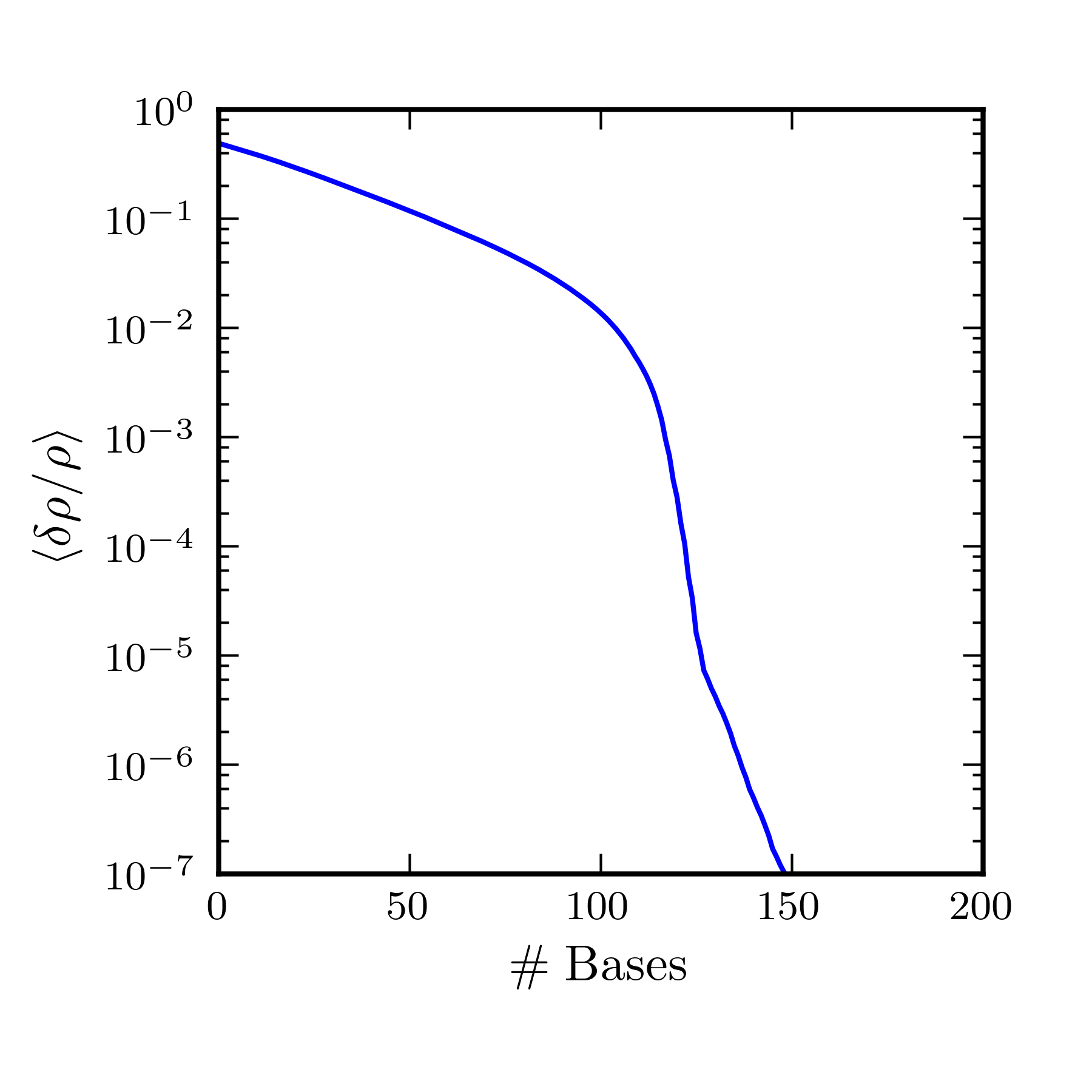
In Fig. 3, we plot δρ/ρdelimited-⟨⟩𝛿𝜌𝜌\langle\delta\rho/\rho\rangle as a function of the number of basis vectors kept. If we require that δρ/ρ=103delimited-⟨⟩𝛿𝜌𝜌superscript103\langle\delta\rho/\rho\rangle=10^{-3}, we find we can reduce the number of filters in the above template bank from N=912𝑁912N=912 to N=118superscript𝑁118N^{\prime}=118, about an order of magnitude reduction in the number of filters.
Refer to caption
Figure 3: The expected fractional SNR loss, δρ/ρdelimited-⟨⟩𝛿𝜌𝜌\langle\delta\rho/\rho\rangle, given by (27) as a function of the number of basis vectors we retain (out of N=912𝑁912N=912). The region δρ/ρ>10%delimited-⟨⟩𝛿𝜌𝜌percent10\langle\delta\rho/\rho\rangle>10\% should be ignored as the Taylor expansion of the fractional SNR loss in (22) is not valid in that regime.

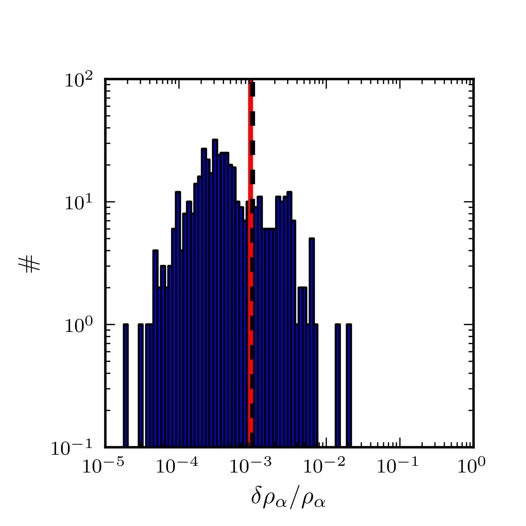
In Fig. 4 we show how δρ/ρdelimited-⟨⟩𝛿𝜌𝜌\langle\delta\rho/\rho\rangle compares to the actual distribution of δρα/ρα𝛿subscript𝜌𝛼subscript𝜌𝛼\delta\rho_{\alpha}/\rho_{\alpha}, where we have chosen random values of ϕitalic-ϕ\phi for each template. We find it is a good measure of the expected fractional loss of SNR.
Refer to caption
Figure 4: Histogram of measured fractional SNR loss, δρα/ρα𝛿subscript𝜌𝛼subscript𝜌𝛼\delta\rho_{\alpha}/\rho_{\alpha}, where we have chosen a random values of ϕitalic-ϕ\phi for each template. The mean value predicted by (27), shown as the dashed-black line, matches the measured mean shown in solid-red.

We have investigated how generic this reduction of filters is for other regions of CBC mass parameter space (e.g., regions of parameter space with larger component masses), and find the reduction to be similar. We tested this by generating a template bank with a 96.8%percent96.896.8\% minimal match, component masses between 1M1subscript𝑀direct-product1M_{\odot} and 34M34subscript𝑀direct-product34M_{\odot}, and total mass below 35M35subscript𝑀direct-product35M_{\odot}. We then ordered the templates by chirp mass, split the template bank up into patches of M=456𝑀456M=456 templates, and computed the SVD for these patches.

We can include larger portions of parameter space in the SVD by including more templates such that the number of templates is smaller than the number of time-samples per template. However the compuational cost of the SVD of an N×L𝑁𝐿N\times L matrix with NL𝑁𝐿N\leq L grows as 𝒪(LN2)𝒪𝐿superscript𝑁2\mathcal{O}(LN^{2}), thus including more templates nonlinearly increases the cost. Another complication is that waveforms further apart in parameter space have smaller overlap. This will result in more basis vectors being required to reconstruct the waveforms to the same accuracy. Therefore, including larger portions of parameter space in a single SVD computation will result in diminishing returns for the computational cost. We propose to address this issue, as above, by breaking up the parameter space into patches for which we can independently compute the SVD, although how best to do this is beyond the scope of the present work.

IV Conclusion

We have investigated how the SVD can be used to reduce the number of filters needed when analyzing GW data for CBC signals. We have found the number of filters required to matched filter these template banks can be reduced by about an order of magnitude through truncating the SVD of these waveforms. This result differs from other work that models CBC GW signals in approximate ways Chassande-Mottin and Pai (2006); Candès et al. (2008); Buonanno et al. (2003) by starting with an exact representation of the desired template family and producing a rigorous approximation with a tunable accuracy.

We plan to explore several topics in future works. Among these are the derivation of a composite detection statistic using only the SVD coefficients in order to minimize the computational costs associated with reconstruction and the interpolation of signals not in the original template set.

Acknowledgements.
The authors would like to acknowledge the support of the LIGO Lab, NSF grants PHY-0653653 and PHY-0601459, and the David and Barbara Groce Fund at Caltech. LIGO was constructed by the California Institute of Technology and Massachusetts Institute of Technology with funding from the National Science Foundation and operates under cooperative agreement PHY-0757058. The authors also thank Stephen Privitera and Ik Siong Heng for useful comments and discussions on this manuscript. This paper has LIGO Document Number LIGO-P1000037-v2.

References

  • Owen (1996) B. J. Owen, Phys. Rev. D 53, 6749 (1996).
  • Owen and Sathyaprakash (1999) B. J. Owen and B. S. Sathyaprakash, Phys. Rev. D 60, 022002 (1999).
  • Brady and Ray-Majumder (2004) P. R. Brady and S. Ray-Majumder, Classical and Quantum Gravity 21, S1839 (2004), URL arXiv:gr-qc/0405036.
  • Heng (2009) I. S. Heng, Classical and Quantum Gravity 26, 105005 (2009), URL http://stacks.iop.org/0264-9381/26/i=10/a=105005.
  • Wen (2008) L. Wen, Int. J. Mod. Phys. D 17, 1095 (2008), URL http://arxiv.org/abs/gr-qc/0702096v2.
  • Croce et al. (2000) R. P. Croce, T. Demma, V. Pierro, I. M. Pinto, and F. Postiglione, Phys. Rev. D 62, 124020 (2000), URL http://link.aps.org/doi/10.1103/PhysRevD.62.124020.
  • Mitra et al. (2005) A. S. Mitra, S. V. Dhurandhar, and L. S. Finn, Phys. Rev. D 72, 102001 (2005).
  • Allen et al. (2005) B. A. Allen, W. G. Anderson, P. R. Brady, D. A. Brown, and J. D. E. Creighton (2005), eprint gr-qc/0509116.
  • Wainstein and Zubakov (1962) L. A. Wainstein and V. D. Zubakov, Extraction of signals from noise (Prentice-Hall, Englewood Cliffs, NJ, 1962).
  • Galassi et al. (2009) M. Galassi, J. Davies, J. Theiler, B. Gough, G. Jungman, P. Alken, M. Booth, and F. Rossi, GNU Scientific Library Reference Manual (Network Theory Ltd, United Kingdom, 2009), 3rd ed., for version 1.12.
  • (11) LSC, URL https://www.lsc-group.phys.uwm.edu/daswg/projects/lal.html.
  • Chassande-Mottin and Pai (2006) E. Chassande-Mottin and A. Pai, Phys. Rev. D 73, 042003 (2006), URL http://arxiv.org/abs/gr-qc/0512137.
  • Candès et al. (2008) E. J. Candès, P. R. Charlton, and H. Helgason, Class. Quant. Grav 25, 184020 (2008), URL http://arxiv.org/abs/0806.4417.
  • Buonanno et al. (2003) A. Buonanno, Y. Chen, and M. Vallisneri, Phys. Rev. D 67, 024016 (2003), erratum-ibid. 74 (2006) 029903(E).