Entanglement verification with finite data
Abstract
Suppose an experimentalist wishes to verify that his apparatus produces entangled quantum states. A finite amount of data cannot conclusively demonstrate entanglement, so drawing conclusions from real-world data requires statistical reasoning. We propose a reliable method to quantify the weight of evidence for (or against) entanglement, based on a likelihood ratio test. Our method is universal in that it can be applied to any sort of measurements. We demonstrate the method by applying it to two simulated experiments on two qubits. The first measures a single entanglement witness, while the second performs a tomographically complete measurement.

Entanglement is an essential resource for quantum information processing, and producing and verifying entangled states is considered a benchmark for quantum experiments (for a sample from the most recent experiments on a wide variety of physical systems, see exp09 ). Several methods for verifying entanglement have been developed (for overviews, see guehne ; elk ). A bipartite state is entangled if it is not separable, and data demonstrate entanglement if there is no separable state that could have generated them. As the number of data , the data are unambiguous, but for finite , only probabilistic conclusions can be drawn. In this Letter, we quantify exactly what can be concluded from finite or small data sets, using a simple and efficient likelihood ratio test.
We demonstrate the method using two simulated experiments on two-qubit systems 111For larger systems, determining whether a given state is entangled is an NP-hard problem. In multi-partite systems, different classes of entanglement exist, but their classification is still an open problem. Our likelihood ratio method applies to any case where the decision is binary: do the data demonstrate entanglement in a particular class or not? So in this paper, the word “separable” can be generalized to “not in the desired entanglement class.”. The first measures just one observable, an entanglement witness Witness . The other performs a tomographically complete measurement. In both cases, we use likelihood ratios to draw direct conclusions about entanglement, rather than estimating the quantum state as an intermediate step. A related technique for testing violation of local realism, and based on empirical relative entropy instead of the likelihood ratio, was proposed by van Dam et al vanDamIEEE05 and applied by Zhang et al Zhang10 .
Likelihood Ratios: Data could have been generated by any one of many i.i.d. states . Each state represents a theory about the system, and the relative plausibility of different states is measured by their likelihood . A state’s likelihood is simply the probability of the observed data given that state,
| (1) |
and states with higher likelihood are more plausible. If the most likely state is separable, the data clearly do not support entanglement. If it is entangled, then we need to ask how convincing the data are – specifically, whether some separable state is almost as plausible. To judge whether there is (even just one) separable state that fits the data, we compare the likelihoods of (i) the most likely separable state, and (ii) the most likely of all states. Letting be the set of separable states, we define
| (2) |
is a likelihood ratio, and
| (3) |
represents the weight of evidence in favor of entanglement 222The factor of may seem arbitrary. Statisticians use this convention because (as defined) is in many circumstances a random variable (see text, below).. To demonstrate entanglement convincingly, an experiment must yield a sufficiently large value for .
A likelihood ratio does not assign a probability to “ is entangled”. Instead, it yields a confidence level. We can determine what values of typically result from measurements on , and how their distribution depends on whether is entangled or separable. If we measure , and no separable state produces with probability higher than , then we have demonstrated entanglement at the confidence level. If an experimentalist plans (before taking data) to calculate and report “ is entangled” only when the data imply confidence, then the probability that he erroneously reports entanglement 333Statisticians call this a “Type I error”. Erroneously rejecting entanglement, even though the experiment is capable of demonstrating entanglement (which is not the same as reporting separability), is a “Type II error”. In entanglement verification one tries to avoid Type I errors and is merely mildly unenthusiastic about Type II errors. is at most .
So, may be (i) entangled, (ii) separable, or (iii) on the boundary. Boundary states are still separable, and they are the hardest separable states to rule out. To demonstrate entanglement at the confidence level, we must show that there is no boundary state for which . It is difficult to make rigorous probabilistic statements about for small . But as , the following analysis becomes exact, and is generally thought to be reliable for GewekeJASA80 .
The distribution of : The set of quantum states is a convex subset of the vector space of trace-1 Hermitian operators, . An entanglement-verification measurement is represented by a POVM (positive operator-valued measure) , in which each operator represents an event that occurs with probability (Born’s rule), and each defines a probability distribution . Data in which appeared times define empirical frequencies , where . Both and can be represented as elements of an -simplex embedded in a vector space . The probabilities in may be linearly dependent (e.g., if , then for all ), and at most of them can be independent (because contains only parameters). We define as the number of independent probabilities.
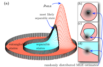
So Born’s rule defines a linear mapping from the operator space containing quantum states into the probability space for measurement . If , then the mapping from states to -vectors is many-to-one, and the experiment is completely insensitive to some parameters of . Ignoring these irrelevant parameters makes an (effectively) -dimensional parameter. Separable states form a convex subset of all states (see Fig. 1). These sets’ images in probability space are also nested convex sets (although if , then some entangled states will be indistinguishable from separable ones in this experiment).
Suppose that copies of a state are measured, yielding a likelihood function . has a unique global maximum . As , the distribution of approaches a Gaussian around with covariance tensor . itself is a Gaussian function with the same covariance matrix (see note 444Technically, this Gaussian ansatz is true only when is full rank – i.e., not on the boundary of the state set. If is rank-deficient, then both the distribution of and itself are typically truncated by the boundary. However, the analysis remains valid (as ) except if is simultaneously rank-deficient and on the boundary between separable and entangled states.). This defines a characteristic length scale that scales as . We can use to define a stretched Euclidean metric
| (4) |
Using this metric, is univariate Gaussian distributed around , and
| (5) |
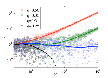
Thus, is determined entirely by , the distance from to the separable set . If is demonstrably entangled, then will grow proportional to – but if it is indistinguishable from a separable state, then will converge almost certainly to zero (see Figure 2).
When is on the boundary, neither grows with nor converges to zero, but continues to fluctuate as . Its distribution is controlled by the shape and radius of , e.g.:
-
1.
If is small w/r.t. , it behaves like a point (see Figure 1b). Then , , and so is a random variable with degrees of freedom (a.k.a. a variable).
-
2.
If is much larger than , then it behaves like a half-space (see Figure 1d and note 555As long as the boundary of is differentiable at .). If were a -dimensional hyperplane, would be a variable. A halfspace behaves like a hyperplane of dimension , except with probability , is separable. Thus, is what we will call a semi- variable: it equals zero with probability , and is -distributed otherwise.
As , case (2) applies. For small , however, the real situation is somewhere in between (see Figure 1c). may be small, and its boundary may be sharply curved, increasing . In the absence of a detailed understanding of ’s shape, case (1) provides the best rigorous upper bound on . Its cumulative distribution is upper bounded by that of a variable – i.e., is no greater than it would be if was a variable. As , the more optimistic semi- ansatz is valid – but only if we know that is “large enough”.
A variable has expected value , and higher values are exponentially suppressed. So is sufficient to demonstrate entanglement at a high confidence level. This implies a tradeoff between an experiment’s power (ability to identify many entangled states) and its efficiency (ability to do so rapidly). Powerful experiments have large dimension – e.g., a tomographically complete measurement can identify any entangled state, but has . This comes at a price; experiments with large dimension are potentially much more prone to spurious large values of , so more data is required to achieve conclusive results []. Conversely, an entanglement witness (see below) is targeted at a particular state, but it can rapidly and conclusively demonstrate entanglement.

Implementation: Computing involves maximizing over two convex sets (the set of all states, and the set of separable states). is log-convex, so in principle this is a convex program.
Testing separability is NP-hard, so efficient minimization over is impossible in general. But for two qubits, the positive partial transpose (PPT) criterion perfectly characterizes entanglement, and can be calculated easily (see examples below). For larger systems, can be bounded by simpler convex sets, as (e.g., PPT states, and convex combinations of specific product states). Maximizing over and yields bounds on , which may (depending on how wisely the bounding sets were chosen) be tight enough to confirm or deny entanglement.
Examples: To demonstrate the likelihood ratio test, we simulate two different experiments on two qubits. We imagine an experimentalist trying to produce the singlet state , and producing instead a Werner state Werner ,
| (6) |
where . Werner states are separable when , and entangled otherwise. The experimentalist’s repeated preparations are assumed to be independently and identically distributed (i.i.d.) renner .

Witness data: The simplest way to test for entanglement is to repeatedly measure a single entanglement witness Witness ; guehne . An optimal witness for Werner states is . Measuring yields one of two outcomes – “yes” or “no” – corresponding to POVM (positive-operator valued measure) elements . The probability of a “yes” outcome is given by Born’s rule as so completely characterizes a state for the purposes of this experiment. The data from measurements is fully characterized by the frequency of “yes” results, . As , represents definitive proof that , and therefore that is entangled. For finite , means that a separable state fits as well as any other, so there is no case for entanglement. When , our likelihood ratio quantifies the weight of the evidence for entanglement. The likelihood function depends only on , as
| (7) | |||||
making this a single-parameter problem. The maximum likelihood, attained at , is , expressed in terms of the data’s empirical entropy,
| (8) |
If , the most likely separable state has , so that which yields
| (9) |
Our numerical explorations (not shown here) confirm that for a barely-separable Werner state, behaves as a semi- variable, even for as low as .
Tomographically complete data: Many entanglement-verification experiments measure a tomographically complete set of observables on a finite-dimensional system (with a heroic example being tomography on 8 ions in an ion trap blatt ). Such data identify uniquely as , so one can determine with certainty whether is entangled (modulo the computational difficulties in determining whether a specified is separable). Analyzing finite data is more complicated than in the witness example, for the data constrain a multidimensional parameter space. Ad-hoc techniques are unreliable, and the likelihood ratio test comes into its own.
We consider an apparatus that applies a SIC (symmetric informationally complete)-POVM sicpovm to each of our two qubits, independently. This measurement (not to be confused with a 4-dimensional SIC-POVM) is tomographically complete, has outcomes, and yields 15 independent frequencies. Unlike , it has no special relationship to Werner states, so any entangled will yield overwhelmingly convincing data as .
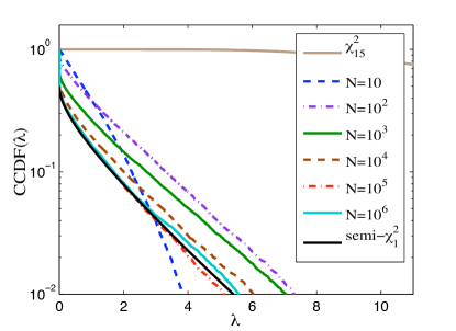
We repeatedly simulated measurements on a barely-separable Werner state (), and compared the empirical distribution of to those of semi- and random variables (see Figure 3). As gets large, becomes indistinguishable from a semi- variable. For smaller , this ansatz is too optimistic (and would produce excessive false positives), but the ansatz is wildly overcautious. We found that for small , behaves like a semi- variable, with a bit larger than 1 (e.g. for ).
Conclusions: Entanglement verification is easy when . In practice, is finite and data are never conclusive. Likelihood ratios provide a simple, reliable test of significance that can be applied to any experimental data. Large values of are very unlikely to be generated by any separable state, but the hardest separable states to rule out are on the boundary. For such states, theory predicts (and our numerics confirm) that behaves like a semi- random variable. If the underlying state is separable, can be upper bounded using a distribution, scaling as for large . For entangled states, grows linearly with , and will thus rapidly become distinguishable from any separable state.
References
- (1) L. Hofstetter et al., Nature 461, 960 (2009); M. Ansmann et al., Nature 461, 504 (2009); E. Amselem and M. Bourennane, Nature Physics 5, 748 (2009); P. Bohi et al., Nature Physics 5, 592 (2009); L. DiCarlo et al., Nature 460, 240 (2009); J. Janousek et al., Nature Photonics 3, 399 (2009); J.D. Jost et al., Nature 459, 683 (2009); J.C.F. Matthews et al., Nature Photonics 3, 346 (2009); A. Fedrizzi et al., Nature Physics 5, 389 (2009); A. Ourjoumtsev et al., Nature Physics 5, 189 (2009); A. S. Coelho et al., Science 326, 823 (2009); Scott B. Papp et al., Science 324 764 (2009); Ryo Okamoto et al., Science 323, 483 (2009); S. Olmschenk et al., Science 323, 486 (2009).
- (2) O. Gühne and G. Toth, Physics Reports 474, 1 (2009).
- (3) S.J. van Enk, N. Lutkenhaus, and H.J. Kimble, Phys. Rev. A 75, 052318 (2007)
- (4) M. Horodecki, P. Horodecki, and R. Horodecki, Phys. Lett. A 223, 1 (1996); B. Terhal, Physics Letters A 271, 319 (2000); P. Hyllus et al., Phys. Rev. A 72, 012321 (2005).
- (5) W. van Dam, R. D. Gill, and P. D. Grunwald, IEEE Trans. Inf. Th. 51, 2812 (2005).
- (6) Y. Zhang, E. Knill, and S. Glancy, arxiv:1001.1750 (2010).
- (7) J. F. Geweke and K. J. Singleton, J. Am. Stat. Assoc., 75, 133 (1980).
- (8) R.F. Werner, Phys. Rev. A 40, 4277 (1989).
- (9) R. Renner, Nature Physics 3, 645 (2007).
- (10) J. M. Renes, R. Blume-Kohout, A. J. Scott, and C. M. Caves, Journal of Mathematical Physics, 45, 2171 (2004).
- (11) H. Häffner et al. Nature 438, 643 (2005).