Memory effect and multifractality of cross-correlations in financial markets

Abstract

Abstract: An average instantaneous cross-correlation function is introduced to quantify the interaction of the financial market of a specific time. Based on the daily data of the American and Chinese stock markets, memory effect of the average instantaneous cross-correlations is investigated over different price return time intervals. Long-range time-correlations are revealed, and are found to persist up to a month-order magnitude of the price return time interval. Multifractal nature is investigated by a multifractal detrended fluctuation analysis.

, , ,

1 Introduction

In recent years, dynamics of financial markets has drawn much attention of physicists [1, 2, 3, 4, 5, 6, 7, 8, 9, 10, 11, 12, 13, 14, 15, 16, 17, 18, 19]. Financial market is a complex system with many interacting components. From the view of many-body systems, interactions among components may lead the system to collective behavior, and therefore result in the so-called dynamic scaling behavior. Based on large amounts of historical data, some stylized facts have been revealed in the past years, such as the ’fat tail’ distribution of the price return, and the long-range time-correlation of the magnitude of returns [1, 10, 11, 12]. Different models and theoretical approaches have been developed to describe financial markets[11, 12, 20, 4, 21, 22, 23, 24].

The cross-correlation function is an important indicator to quantify the interaction between stocks, and therefore has attracted much attention of physicists in recent years. Random and nonrandom properties of the cross-correlation and the relevant economic sectors are revealed [25, 26, 17, 27, 28, 5, 29, 30, 31, 32, 33]. Correlation-based hierarchical or network structures are studied with the graph or complexity theory [34, 35, 36, 37, 38, 39, 40]. The so-called pull effect is found with a time-dependent cross-correlation function [41]. These lines of work are mainly based on a static definition of the cross-correlation function. The equal-time or the time-dependent cross-correlation is usually defined as $C_{ij}={<r_{i}(t^{\prime})r_{j}(t^{\prime})>}$ or $C_{ij}={<r_{i}(t^{\prime})r_{j}(t^{\prime}+\tau)>}$, with $r_{i}(t^{\prime})=lny_{i}(t^{\prime}+\Delta t^{\prime})-lny_{i}(t^{\prime})$ being the return of stock $i^{\prime}s$ price $y_{i}$ over a time interval $\Delta t^{\prime}$, $\tau$ being the time lag, and $<...>$ taking time average over $t^{\prime}$. The static cross-correlation function can not reveal the dynamic behavior of the cross-correlations between stocks. More recently, a Detrended Cross-Correlation Analysis(DCCA) is proposed to investigate the memory effect of the cross-correlations between two time series [42, 43, 44, 45]. Long-range time-correlation of the cross-correlations is characterized by a power-law scaling of the DCCA function. The DCCA method concentrates on dynamics of two series’ cross-correlations.

In this paper, we introduce an Instantaneous Cross-correlation($IC$) and an Average Cross-correlation($AIC$) function by considering the cross-correlations of a single time step. The $IC$ and $AIC$ function describes the current interaction between stocks with local information. Our purpose is to investigate the dynamics of the $IC$ and $AIC$ series, based on the daily data of the American and Chinese stock markets. More importantly, we examine the memory effect of the $AIC$ over different price return time intervals. The multifractal nature of the $AIC$ is also revealed.

The organization of this paper is as follows. In the next section, the datasets and the definition of the $IC$ and $AIC$ functions are presented. In Sec. 3, we investigate the memory effect of the $IC$ and $AIC$ for a shorter price return time interval. In Sec. 4, the memory effect of the $AIC$ is detected over different scales of price return time intervals. In section 5, we examine the multifractal nature of the $AIC$. Finally, Sec. 6 contains the conclusion.

2 datasets and instantaneous cross-correlations

To obtain a comprehensive study, we analyze two different databases, the New York Stock Exchange (NYSE) and the Chinese Stock Market(CSM). The two markets cover the mature and the emerging markets. The NYSE is one of the oldest stock exchanges, whereas the CMS is a newly set up market in $1990$. We investigate the daily data of $249$ individual stocks, with $2900$ data points from the year $1997$ to $2008$ for the NYSE, and the daily data of $259$ individual stocks, with $2633$ data points from the year $1997$ to $2007$ for the CSM. To compare different stocks, we define the normalized the price return as

$$R_{i}(t^{\prime},\Delta t^{\prime})={\frac{r_{i}(t^{\prime})-<r_{i}(t^{\prime})>}{\sigma_{i}}}$$ (1)

where $r_{i}(t^{\prime})$ is the price return of stock $i$ at time $t^{\prime}$, and $\Delta{t^{\prime}}$ is the price return time interval. The $\sigma_{i}={\sqrt{<r_{i}^{2}>-<r_{i}>^{2}}}$ is the standard deviation of $r_{i}$, and $<\ldots>$ takes time average over $t^{\prime}$. In order to quantify the current cross-correlation between stocks, we introduce an $IC$ function between two stocks by

$$IC_{ij}(t^{\prime})=R_{i}(t^{\prime})R_{j}(t^{\prime}),$$ (2)

The $IC$ function indicates the instantaneous cross-correlation between two individual stocks. However, it does not depict the average interaction of the financial market. Therefore, we define an $AIC$ function as

$$AIC(t^{\prime})=\frac{2}{N(N-1)}\sum_{i=1}^{N-1}\sum_{j=i+1}^{N}C_{ij}(t^{\prime})$$ (3)

where $N$ is the number of stocks. The $AIC$ function indicates the average instantaneous cross-correlation of a number of stocks with the stock size to be $N$. As the stock number $N$ is large enough, the $AIC$ function can be then considered as an indicator to quantify the average interaction of the financial market at a specific time step. For $N=2$, the $AIC$ function reduces to the $IC$ function.

3 Memory effect of $IC$ and $AIC$ for a shorter $\Delta t^{\prime}$

It is important to measure the memory effect of the time series during the dynamic evolution. We investigate the memory effect of the $IC$ and $AIC$ by computing the time-correlations. The autocorrelation function is widely adopted to measure the time-correlation. However, it shows large fluctuations for nonstationary time series. Therefore, we apply the DFA method [46, 47].

Considering a fluctuating dynamic series $A(t^{\prime})$, one can construct

$$B(t^{\prime})=\sum\limits_{t"=1}^{t^{\prime}}A(t"),$$ (4)

Dividing the total time interval into windows $N_{t}$ with a size of $t$, and linearly fit $B(t^{\prime})$ to a linear function $B_{t}(t^{\prime})$ in each window. The DFA function of the $k_{th}$ window box is then defined as:

$$f_{k}(t)^{2}=\frac{1}{t}\sum\limits_{t^{\prime}=(k-1)t+1}^{kt}{[B(t^{\prime})-B_{t}(t^{\prime})]}^{2},$$ (5)

The overall detrended fluctuation is estimated as

$$F_{2}(t)^{2}=\frac{1}{N_{t}}\sum\limits_{k=1}^{N_{t}}{[f_{k}(t)]}^{2},$$ (6)

In general, $F_{2}(t)$ will increase with the window size $t$ and obey a power-law behavior $F_{2}(t)\sim t^{H}$. If $0.5<H<1.0$, $A(t^{\prime})$ is long-range correlated in time; if $0<H<0.5$, $A(t^{\prime})$ is temporally anti-correlated; $H=0.5$ corresponds to the Gaussian white noise, while $H=1.0$ indicates the $1/f$ noise. If $H$ is bigger than $1.0$, the time series is considered to be unstable.

The DFA functions of the $IC$ and the $AIC$ are computed with the price return time interval $\Delta t^{\prime}=1$ day. To illustrate the results, we take $6$ $ICs$ and $AICs$ as examples, with the stocks randomly chosen from the NYSE and the CSM, respectively. As shown in Fig. 1(a), the DFA exponents of the $ICs$ are estimated to be from $0.46$ to $0.65$ for the NYSE. The exponent $0.46$ is close to the Gaussian behavior, while $0.65$ is the long-range correlation. Similarly, as shown in Fig. 1(c) for the $ICs$ of the CSM, the DFA exponents range from $0.53$ to $0.67$, also corresponding to the Gaussian behavior and the long-range correlation, respectively. It suggests that the long-range time-correlation does not hold for all $ICs$. However, when we compute the DFA of the $AIC$, robust long-range time-correlations are observed for both the NYSE and the CSM. As shown in Fig. 1(b) and (d), the DFA functions of 6 $AICs$ are shown as examples with $N=50$. The DFA exponents are estimated to be around 0.73 for the NYSE, and 0.67 for the CSM, both in the long-range time-correlation range $(0.5,1.0)$. The DFA exponents of the $AIC$ take the similar value for a larger stock number $N$ from our databases. It implies that, for both the NYSE and the CSM, even though the absence of the long-range time-correlation of the instantaneous cross-correlation between two individual stocks, the average instantaneous cross-correlation of a number of stocks is long-range correlated, i.e., the average interaction of the financial market shows long-term memory. The result is reasonable. For example, it is possible for two correlated companies to break up their relationship during the time evolution for some reason. With the end of the correlation, the memory of the cross-correlation then also ends up. However, the fluctuation from the endogenous events would not influence the average interaction of the whole market, i.e., as a collective, the cross-correlation of the financial market is always characterized by a long-range memory.

4 Memory effect of $AIC$ for different $\Delta t^{\prime}$

Scalings observed in the financial market has been found to always evolve with the different value of the price return intervals. For example, the ’fat tail’ of the probability density function of the price returns can not be found for a big return time interval [10]. To further understand the memory effect of the cross-correlations, we then investigate the DFA functions of the $AIC$ with different price return time interval $\Delta t^{\prime}$. The return time interval $\Delta t^{\prime}$ covers three magnitude orders, the day, the week and the month time scales.

The $AIC$ is computed with $N=249$ for the NYSE, and $N=259$ for the CSM. In Fig. 2(a), the DFA function of the $AIC$ is shown for the NYSE, with $\Delta t^{\prime}=1$, $5$, $10$, $22$, and $44$ days, approximate to a working day, a week, half a month, a month, and two months. For $\Delta t^{\prime}=1$ day, clean power-law behavior is observed, with the exponent estimated to be $0.74$, consistent with the exponents obtained in Fig. 1. For the return time interval $\Delta t^{\prime}$ bigger than $1$ day, two-stage power-law scalings are observed, with a crossover in between. Such a two-stage behavior has been widely found in the DFA function of the financial series, such as the volatilities, intertrade durations, etc [48, 49, 50]. The crossover time is about $t_{c}\sim 35$ days. For the smaller window size, the DFA exponents take the value around $1.0$ for $\Delta t^{\prime}=5$, and bigger than the 1.0 for $\Delta t^{\prime}=10$, $22$ days, which correspond to the $1/f$ noise and unstable time series, respectively. Due to the narrow range of the smaller window size, we care more about the DFA exponents of the larger window size. For the larger window size from $t=35$ to 100 days, the exponents are measured to be $0.65$, $0.72$, $0.86$ for $\Delta t^{\prime}=5$, $10$ and $22$ days, with all the exponent value ranged in the long-range time-correlation. The estimated exponents also remain unchanged for a relatively larger window size than 100 days. However, due to the finite size of the time series, it will show large fluctuation for a large window size. For $\Delta t^{\prime}=44$ days, both the smaller and the larger window size do not show long-range time-correlations. Therefore, the long-range time-correlation of the $AIC$ persists up to a working month magnitude of the price return time interval for the NYSE for the large window size. Similar behavior is also observed for the CSM. For $\Delta t^{\prime}=1$ day, clean power-law behavior is observed, with the exponent estimated to be 0.68, around 0.67 found in Fig. 1. Also, two-stage power-law scalings are observed for $\Delta t^{\prime}=5$, $10$ days, with the smaller window size showing $1/f$ noise and unstable time series, and the larger window size showing long-range time-correlations. The cross-over time $t_{c}\sim 22$ days. The long-range memory persists up to half a month magnitude of the price return time interval for the CSM for the larger window size.

5 multifractal nature of $AIC$

Financial time series such as the price returns and the intertrade durations has been revealed to present multifractal feature [50, 51, 52]. The multifractal detrended fluctuation analysis(MF-DFA) has been successfully applied to detect multifractal characteristic of nonstationary time series [53]. We then apply the MF-DFA into the $AIC$, with $N=249$ for the NYSE, and $N=259$ for the CSM. The MF-DFA is a generalization of the DFA method by considering different order of detrended fluctuation. For the $q_{th}$ order of the detrended fluctuation, we have

$$F_{q}(t)=\{\frac{1}{N_{t}}\sum_{k=1}^{N_{t}}[f_{k}(t)]^{q}\}^{1/q},$$ (7)

where $q$ can take any real number except $q=0$. For $q=0$, we have

$$F_{0}(t)=\exp\{\frac{1}{N_{t}}\sum_{k=1}^{N_{t}}\ln[f_{k}(t)]\},$$ (8)

The MF-DFA function $F_{q}(t)$ scales with the window size $t$:

$$F_{q}(t)\sim t^{h(q)},$$ (9)

where $h(q)$ is the MF-DFA exponent, with $q=2$ recovering the DFA exponent. Due to the finite size of the time series, the $F_{q}(t)$ shows large fluctuations for the large values of $|q|$. Here we take $q\in[-2,4]$, and $\Delta t^{\prime}=1$ day as examples to show the multifractal properties. The $F_{q}(t)$ of the $AIC$ is shown for the NYSE and CSM in Fig. 3. Clean power law scalings are observed for $q=-2$, $0$, $2$ and $4$, with the exponents estimated to be $1.13$, $0.95$, $0.68$, $0.52$ for the NYSE, and $0.89$, $0.84$, $0.74$,$0.57$ for the CSM. The dependence of the $F_{q}(t)$ on $q$ suggests that the $AIC$ shows a multifractal characteristic. The MF-DFA exponent $h(q)$ versus different $q$ is shown in Fig. 4(a) and (d), respectively for the NYSE and the CSM.

The scaling exponent function $\tau(q)$ based on partition function is widely adopted to reveal the multifractality,

$$\tau(q)=qh(q)-D_{f},$$ (10)

where $D_{f}$ is the fractal dimension, with $D_{f}=1$ in our case. As shown in Fig. 4(b) and (e), the $\tau(q)$ of the NYSE and the CSM presents a strong nonlinearity, which is consistent with multifractal characteristic. By the Legendre transformation, the local singularity exponent $\alpha$ and its spectrum $f(\alpha)$ can be calculated as [54],

$$\alpha=d\tau(q)/dq,$$ (11)

$$f(\alpha)=q\alpha-\tau(q),$$ (12)

The difference between the maximum and the minimum of the local singularity exponent $\Delta\alpha\triangleq\alpha_{max}-\alpha_{min}$ is widely used to quantify the width of the extracted multifractal spectrum. The larger the $\Delta\alpha$, the stronger the multifractality. Fig. 4(c) and Fig. 4(f) illustrate the multifractal singularity spectra $f(\alpha)$, with the width of the extracted multifractal spectrum $\Delta\alpha$ measured to be $0.64$ and $0.93$ respectively for the NYSE and the CSM. It indicates the CSM shows stronger multifractality than the NYSE.

6 Conclusion

We have investigated the memory effect of the instantaneous cross-correlations and the average instantaneous cross-correlations based on the daily data of the NYSE and the CSM. It is interesting to find that, in spite of the absence of the long-range time-correlation of the instantaneous cross-correlations between two individual stocks, the average instantaneous cross-correlation of a set of stocks is long-range correlated for the price return time interval $\Delta t^{\prime}=1$ day. The long-range time-correlation persists up to a month price return time interval for the NYSE, and half a month time interval for the CSM for the large time window.

Multifractal nature is revealed for the average instantaneous cross-correlations by the MF-DFA. By examining the MF-DFA function $F_{q}(t)$, the scaling exponent function $\tau(q)$, and the extracted multifractal spectrum $f(\alpha)$, multifractal features are revealed for both the NYSE and the CSM.

Acknowledgments:

This work was supported by the National Natural Science Foundation of China (Grant Nos. 10805025, 10774080) and the Foundation of Jiangxi Educational Committee of China.

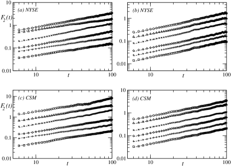
Figure 1: The DFA functions of the $IC$ and the $AIC$ are displayed on a log-log scale, with the circles, triangles, crosses, diamonds, pluses and squares being six samples. The dashed lines are the power law fits. For clarity, some curves have been shifted downwards or upwards.(a) for the $IC$ of the NYSE. The exponents are measured to be $0.61$, $0.46$, $0.65$, $0.60$, $0.49$ and $0.52$. (b) for the $AIC$ of the NYSE with $N=50$. The exponents are measured to be $0.73$, $0.71$, $0.75$, $0.71$, $0.73$ and $0.73$. (c) for the $IC$ of the CSM. The exponents are measured to be $0.61$, $0.67$, $0.63$, $0.59$, $0.53$ and $0.58$. (d) for the $AIC$ of the CSM with $N=50$. The exponents are measured to be $0.67$, $0.68$, $0.67$, $0.68$, $0.66$ and $0.67$.

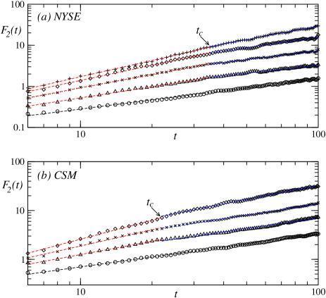
Figure 2: The DFA functions of the $AIC$ are displayed on a log-log scale, with the dashed lines being the power law fits. Some curves have also been shifted downwards or upwards for clarity. (a) For the NYSE and $N=249$, the circles, triangles, crosses, diamonds, and pluses are for $\Delta t^{\prime}=1$, $5$, $10$, $22$, and $44$ days, respectively. The power-law exponent for $\Delta t^{\prime}=1$ day is measured to be $0.74$ for the whole window size. Two stage power-law exponents for $\Delta t^{\prime}=5$, $10$, $22$ and $44$ days are respectively measured to be $0.91$, $1.08$, $1.23$, $1.31$ for the smaller window size, and $0.65$, $0.72$, $0.86$, $1.08$ for the larger window size. (b)For the CSM and $N=259$, the circles, triangles, crosses, and diamonds are for $\Delta t^{\prime}=1$, $5$, $10$, and $22$ days, respectively. The power-law exponent for $\Delta t^{\prime}=1$ day is measured to be $0.68$ for the whole window size. Two stage power-law exponents for $\Delta t^{\prime}=5$, $10$ and $22$ days are respectively measured to be $0.90$, $1.09$, $1.29$ for the smaller window size, and $0.72$, $0.76$, $0.95$ for the larger window size.

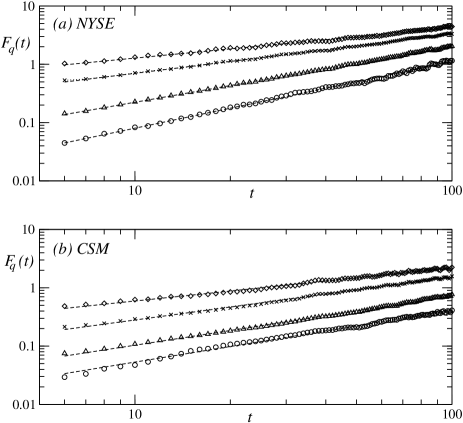
Figure 3: The MF-DFA functions of the $AIC$ are displayed on a log-log scale, with the dashed lines being the power law fits. The circles, triangles, crosses and diamonds are for $q=-2$, $0$, $2$ and $4$, with curves being shifted downwards or upwards for clarity. (a) For the NYSE and $N=249$, with the exponents estimated to be $1.13$, $0.95$, $0.68$, and $0.52$. (b) For the CSM and $N=259$, with the exponents estimated to be $0.89$, $0.84$, $0.74$, and $0.57$.

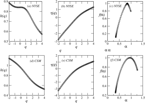
Figure 4: The multifractal analysis of the $AIC$ is displayed with $N=249$ for the NYSE and $N=259$ for the CSM. (a) and (d) are the MF-DFA exponents $h(q)$ versus $q$ for the NYSE and the CSM. (b) and (e) are the scaling exponent function $\tau(q)$ for the NYSE and the CSM. (c) and (f) are the multifractal spectrum $f(\alpha)$ for the NYSE and the CSM.

References

- [1] R.N. Mantegna and H.E. Stanley, Nature 376 (1995) 46.
- [2] R.N. Mantegna and H.E. Stanley, Nature 383 (1996) 587.
- [3] S. Ghashghaie et al., Nature 381 (1996) 767.
- [4] D. Stauffer, P.M.C. de Oliveria and A.T. Bernardes, Int. J. Theor. Appl. Financ. 2 (1999) 83.
- [5] L. Laloux et al., Phys. Rev. Lett. 83 (1999) 1467.
- [6] B.M. Roehner, Int. J. Mod. Phys. C 11 (2000) 91.
- [7] B.M. Roehner, Int. J. Mod. Phys. C 12 (2001) 43.
- [8] J. Bouchaud, A. Matacz and M. Potters, Phys. Rev. Lett. 87 (2001) 228701.
- [9] H.E. Stanley et al., Physica A 299 (2001) 1.
- [10] P. Gopikrishnan et al., Phys. Rev. E 60 (1999) 5305.
- [11] T. Lux and M. Marchesi, Nature 397 (1999) 498.
- [12] I. Giardina, J.P. Bouchaud and M. Mézard, Physica A 299 (2001) 28.
- [13] T. Qiu et al., Phys. Rev. E 73 (2006) 065103.
- [14] T. Qiu, L. Guo and G. Chen, Physica A 387 (2008) 6812.
- [15] T. Qiu et al., Physica A 388 (2009) 2427.
- [16] F. Ren and W.X. Zhou, EPL 84 (2008) 68001.
- [17] J. Shen and B. Zheng, Europhys. Lett. 86 (2009) 48005.
- [18] J. Shen and B. Zheng, Europhys. Lett. 88 (2009) 28003.
- [19] B. Tóth and J. Kertész, Physica A 360 (2006) 505.
- [20] D. Challet and Y.C. Zhang, Physica A 246 (1997) 407.
- [21] R. Cont and J.P. Bouchaud, Macroeconomic Dyn. 4 (2000) 170.
- [22] V.M. Eguiluz and M.G. Zimmermann, Phys. Rev. Lett. 85 (2000) 5659.
- [23] F. Ren et al., Physica A 371 (2006) 649.
- [24] F. Ren et al., Phys. Rev. E 74 (2006) 041111.
- [25] V. Plerou et al., Phys. Rev. E 66 (2002) 027104.
- [26] C. Coronnello et al., Acta Phys. Pol. B 36 (2005) 2653.
- [27] A. Utsugi, K. Ino and M. Oshikawa, Phys. Rev. E 70 (2004) 026110.
- [28] A. Garas, P. Argyrakis and S. Havlin, Eur. Phys. J. B 63 (2008) 265.
- [29] V. Plerou et al., Phys. Rev. Lett. 83 (1999) 1471.
- [30] V. Plerou et al., Phys. Rev. E 62 (2000) R3023.
- [31] V. Plerou et al., Quant. Finance 1 (2001) 262.
- [32] B. Rosenow et al., Physica A 324 (2003) 241.
- [33] T. Conlon, H.J. Ruskina and M. Crane, Physica A 388 (2009) 705.
- [34] R.N. Mantegna, Eur. Phys. J. B 11 (1999) 193.
- [35] G. Bonanno et al., Phys. Rev. E 68 (2003) 046130.
- [36] M. Tumminello et al., Proc. Natl. Acad. Sci. USA 102 (2005) 10421.
- [37] M. Tumminello et al., Eur. Phys. J. B 55 (2007) 209.
- [38] C. Eom, G. Oh and S. Kim, Physica A 383 (2007) 139.
- [39] M. Eryigit and R. Eryigit, Physica A 388 (2009) 3551.
- [40] T. Qiu, B. Zheng and G. Chen, arXiv:1002.3432 (2010).
- [41] L. Kullmann, J. Kertész and K. Kaski, Phys. Rev. E 66 (2002) 026125.
- [42] B. Podobnik et al., Physica A 387 (2008) 3954.
- [43] B. Podobnik and H.E. Stanley, Phys. Rev. Lett. 100 (2008) 084102.
- [44] B. Podobnik et al., Proc. Natl. Acad. Sci. USA 106 (2009) 22079.
- [45] B. Podobnik et al., Eur. Phys. J. B 71 (2009) 243.
- [46] C.K. Peng et al., Phys. Rev. E 49 (1994) 1685.
- [47] C.K. Peng et al., Chaos 5 (1995) 82.
- [48] Y. Liu et al., Phys. Rev. E 60 (1999) 1390.
- [49] T. Qiu et al., Physica A 378 (2007) 387.
- [50] Z.Q. Jiang and W.X. Zhou, Physica A 387 (2008) 4881.
- [51] Z.Q. Jiang and W.X. Zhou, Physica A 387 (2008) 3605.
- [52] W.X. Zhou, EPL 88 (2009) 28004.
- [53] J.W. Kantelhardt et al., Physica A 316 (2002) 87.
- [54] L.T.C. Halsey et al., Phys. Rev. A 33 (1986) 1141.