Self-consistent electron counting statistics

Abstract

We develop a self-consistent version of perturbation theory in Liouville space which seeks to combine the advantages of master equation approaches in quantum transport with the nonperturbative features that a self-consistent treatment brings. We describe how counting fields may be included in a self-consistent manner in this formalism such that the full counting statistics can be calculated. NonMarkovian effects are also incorporated. Several different self-consistent approximations are introduced and we discuss their relative strengths with a simple example.

I Introduction

Master equation (ME) techniques play an important role in quantum transport — not only in describing state-of-the-art experiments e.g. Sukh07 ; fri07 ; shi09 ; fli09 ; nad10 , but also in contributing to the theoretical development of the field; topics such as full counting statistics (FCS), both at zero bag03 and finite EMAB07 frequency; quantum coherent phenomena bra05 ; and nonMarkovian (NM) effects bra06 ; fli08 have all been investigated with master equations. The central object in such approaches is the Liouvillian or kernel, which generates the evolution of the reduced system density matrix in time and includes not only the internal dynamics of the system but also the effects of the coupling to the leads and to any further environmental degrees of freedom. ME Liouvillians can be derived in a number of different ways, from the standard textbook approaches, e.g. coh92 ; breu02 , to more transport-specific ones such as the wavefunction approach of Gurvitz gur96 , and the real-time diagrams sch94 ; kon96 ; thi03 ; thi05 . A reformulation of this latter approach, the Liouvillian perturbation theory (LPT)sch08 ; lei08 ; ce09 , will form the basis of the current work.

Despite their many advantages, standard ME approaches are restricted to the regime in which system and environment are but weakly coupled, with the Liouvillian obtained as a perturbation series in the corresponding coupling strength. There is much interest in going beyond this situation and to develop nonperturbative approaches for the description of quantum transport beyond the ME. Some recent examples include equations of motion ped05 , renormalisation group kor07 and self-consistent cui06 ; esp10 techniques.

In this paper we develop a self-consistent (SC) version of the LPT, which seeks to combine the advantages of MEs with a nonperturbative treatment of the system-lead coupling such that effects such as, for example, level-broadening and higher-order tunnel processes are included. The method is self-consistent in the sense that system self-energies are calculated not with free propagators, but rather with ones that include the self-energy itself. We describe how counting fields may be included in a self-consistent manner in this formalism, which means that we are not restricted to the calculation of stationary current only (as in, e.g. cui06 ), but can, in principle, access the complete FCS of the system. NonMarkovian (NM) effects are also included in our theory from the outset.

Within this framework, we introduce several different SC approximations. The simplest of these is just a SC version of the familiar sequential-tunneling kernel. This approximation is equivalent to the SC Born approximation bru04 , appearing in a setting similar to that of Ref. cui06 . By considering the single-resonant level (SRL) model as a test case, we see that although this type of kernel can provide an excellent description of the stationary current even for large couplings ($\Gamma/k_{B}T\gg 1$) it gives inaccurate results for the shotnoise, and is unsuitable for the calculation of counting statistics in general. The problems of this kernel are remedied to some extent by the other two kernels described here, which contain not only sequential-type diagrams, but also cotunneling ones. With these kernels excellent results are obtainable for both current and shotnoise beyond weak coupling.

This work is based on the exposition of the LPT given in Ref. ce09 , hereafter referred to as I. To save needless repetition, the reader will be this paper for many of the details of the original LPT and the notation employed here.

II Transport Model

We begin by specifying our general transport model with the Hamiltonian $H=H_{\mathrm{res}}+H_{\mathrm{S}}+V$ composed of reservoir, system, and interaction parts. In its diagonal basis the system part reads $H_{\mathrm{S}}=\sum_{a}E_{a}|a\rangle\langle a|$ with $|a\rangle$ a many-body state of $N_{a}$ electrons. We assume a noninteracting reservoir Hamiltonian $H_{\mathrm{res}}=\sum_{k,\alpha}(\omega_{k\alpha}+\mu_{\alpha})a^{\dagger}_{k\alpha}a_{k\alpha}$, with lead index $\alpha$ that includes spin and any other relevant quantum numbers; $\omega_{k\alpha}$ is the energy of the $k$th mode in lead $\alpha$, $a_{k\alpha}$ a lead annihilation operator, and with $\mu_{\alpha}$ the chemical potential of lead $\alpha$. In equilibrium, the reservoir electrons are distributed according to the Fermi function $f(\omega)=1/\left(e^{\omega/k_{B}T}+1\right)$, which, since we assume a uniform temperature, is the same for all reservoirs. Coupling between system and reservoirs is described by the single-particle tunneling Hamiltonian

$$V=\sum_{k\alpha m}t_{k\alpha m}a^{\dagger}_{k\alpha}d_{m}+t^{*}_{k\alpha m}d^{\dagger}_{m}a_{k\alpha},$$ (1)

where $d_{m}$ is the annihilation operator for single-particle level $m$ in the system, and $t_{k\alpha m}$ is a tunneling amplitude.

III Self-consistent Liouvillian perturbation theory

For completeness we give a brief review of the essential elements of the standard Liouvillian perturbation theory — for more details, the reader is referred I as well as to sch08 ; lei08 . Our starting point is to write down the von Neumann equation for the evolution of the total system-plus-reservoirs density matrix:

$$\dot{\rho}(t)=-i\left[H,\rho(t)\right]={\cal L}\rho(t).$$ (2)

This defines the Liouvillian super-operator ${\cal L}=-i\left[H,\bullet~{}\right]$, which, in accordance with the decomposition of the Hamiltonian, consists of three parts: ${\cal L}={\cal L}_{\mathrm{res}}+{\cal L}_{\mathrm{S}}+{\cal L}_{V}$ with ${\cal L}_{\mathrm{res}}=-i\left[H_{\mathrm{res}},\bullet~{}\right]$, ${\cal L}_{\mathrm{S}}=-i\left[H_{\mathrm{S}},\bullet~{}\right]$, and ${\cal L}_{V}=-i\left[V,\bullet~{}\right]$. In terms of the Laplace-transformed total density matrix $\rho(z)=\int_{0}^{\infty}dte^{-zt}\rho(t)$, the solution of Eq. (2) is

$$\rho(z)=\frac{1}{z-{\cal L}}\rho(0).$$ (3)

Assuming a factorizable initial density matrix $\rho(0)$ with reservoirs in equilibrium and system in state $\rho_{\mathrm{S}}(0)$, tracing over reservoir degrees of freedom results in the following reduced density matrix of the system:

$$\rho_{\mathrm{S}}(z)=\mathrm{Tr}_{\mathrm{res}}\left\{\rho(z)\right\}=\frac{1}{z-{\cal W}(z)}\rho_{\mathrm{S}}(0),$$ (4)

with the effective system Liouvillian ${\cal W}(z)={\cal L}_{\mathrm{S}}+\Sigma(z)$. The self-energy $\Sigma(z)$ arises from the coupling with the leads and will be kept in its $z$-dependent nonMarkovian form.

Equation (4) is exact if kernel ${\cal W}(z)$ is. In practice, however, the self-energy contains an infinite sum of terms and must be approximated in some way. In the straightforward perturbative approach, the memory kernel is calculated as the series $\Sigma(z)=\sum_{n}\Sigma^{(n)}(z)$, with $n$ the number of tunnel vertices in the term, and then approximated by simple truncation at a certain value of $n$. In previous works, expansion has been considered up to fourth order, such that the self-energy is approximated as

$$\Sigma(z)\approx\Sigma^{(2)}(z)+\Sigma^{(4)}(z),$$ (5)

with the first term describing sequential tunneling and the second, cotunneling.

In describing the constituent terms of the self-energy and the various modifications to follow, it is useful to employ a diagrammatic representation. In this representation, we write the sequential self-energy term as

$$\Sigma^{(2)}(z) = \mathchoice{\vbox{\hbox to0.0pt{\kern 0.0pt\kern 3.93124pt\hbox{\vrule width=0.50003pt,height=0.0pt,depth=4.30554pt\vrule width=18.50829pt,height=0.0pt,depth=0.50003pt\vrule width=0.50003pt,height=0.0pt,depth=4.30554pt}\hss}\vskip 2.15277pt\vskip 6.83331pt}}{\vbox{\hbox to0.0pt{\kern 0.0pt\kern 3.93124pt\hbox{\vrule width=0.50003pt,height=0.0pt,depth=4.30554pt\vrule width=18.50829pt,height=0.0pt,depth=0.50003pt\vrule width=0.50003pt,height=0.0pt,depth=4.30554pt}\hss}\vskip 2.15277pt\vskip 6.83331pt}}{\vbox{\hbox to0.0pt{\kern 0.0pt\kern 2.75186pt\hbox{\vrule width=0.50003pt,height=0.0pt,depth=4.30554pt\vrule width=11.40027pt,height=0.0pt,depth=0.50003pt\vrule width=0.50003pt,height=0.0pt,depth=4.30554pt}\hss}\vskip 2.15277pt\vskip 4.78333pt}}{\vbox{\hbox to0.0pt{\kern 0.0pt\kern 1.96562pt\hbox{\vrule width=0.50003pt,height=0.0pt,depth=4.30554pt\vrule width=8.14304pt,height=0.0pt,depth=0.50003pt\vrule width=0.50003pt,height=0.0pt,depth=4.30554pt}\hss}\vskip 2.15277pt\vskip 3.41666pt}}G\underset{z}{-}G.$$ (6)

The translation of this diagram into an analytical expression is discussed in Appendix A. Here it suffices to note that the $G$s represent tunnel vertices (of which there are two at sequential order) and these are connected by a single central line that corresponds to the free propagation of the system (i.e. under the action of free system Liouvillian ${\cal L}_{\mathrm{S}}$). The overline connecting the tunnel vertices denotes a bath contraction between them. Such diagrams are similar to those of Ref. lei08 , but simplified such that we leave the indices implicit here.

At fourth order in the perturbative expansion of the self-energy there are two diagrams, each with four tunnel vertices and three free propagators, but with differing patterns of contraction. In our diagrammatic notation, we write

$$\Sigma^{(4)}(z)=\mathchoice{\vbox{\hbox to0.0pt{\kern 0.0pt\kern 3.93124pt\hbox{\vrule width=0.50003pt,height=0.0pt,depth=8.61108pt\vrule width=55.52486pt,height=0.0pt,depth=0.50003pt\vrule width=0.50003pt,height=0.0pt,depth=8.61108pt}\hss}\vskip 2.15277pt\vskip 6.83331pt}}{\vbox{\hbox to0.0pt{\kern 0.0pt\kern 3.93124pt\hbox{\vrule width=0.50003pt,height=0.0pt,depth=8.61108pt\vrule width=55.52486pt,height=0.0pt,depth=0.50003pt\vrule width=0.50003pt,height=0.0pt,depth=8.61108pt}\hss}\vskip 2.15277pt\vskip 6.83331pt}}{\vbox{\hbox to0.0pt{\kern 0.0pt\kern 2.75186pt\hbox{\vrule width=0.50003pt,height=0.0pt,depth=8.61108pt\vrule width=34.2008pt,height=0.0pt,depth=0.50003pt\vrule width=0.50003pt,height=0.0pt,depth=8.61108pt}\hss}\vskip 2.15277pt\vskip 4.78333pt}}{\vbox{\hbox to0.0pt{\kern 0.0pt\kern 1.96562pt\hbox{\vrule width=0.50003pt,height=0.0pt,depth=8.61108pt\vrule width=24.42911pt,height=0.0pt,depth=0.50003pt\vrule width=0.50003pt,height=0.0pt,depth=8.61108pt}\hss}\vskip 2.15277pt\vskip 3.41666pt}}\mathchoice{\vbox{\hbox to0.0pt{\kern 18.50829pt\kern 3.93124pt\hbox{\vrule width=0.50003pt,height=0.0pt,depth=4.30554pt\vrule width=18.50829pt,height=0.0pt,depth=0.50003pt\vrule width=0.50003pt,height=0.0pt,depth=4.30554pt}\hss}\vskip 2.15277pt\vskip 6.83331pt}}{\vbox{\hbox to0.0pt{\kern 18.50829pt\kern 3.93124pt\hbox{\vrule width=0.50003pt,height=0.0pt,depth=4.30554pt\vrule width=18.50829pt,height=0.0pt,depth=0.50003pt\vrule width=0.50003pt,height=0.0pt,depth=4.30554pt}\hss}\vskip 2.15277pt\vskip 6.83331pt}}{\vbox{\hbox to0.0pt{\kern 11.40027pt\kern 2.75186pt\hbox{\vrule width=0.50003pt,height=0.0pt,depth=4.30554pt\vrule width=11.40027pt,height=0.0pt,depth=0.50003pt\vrule width=0.50003pt,height=0.0pt,depth=4.30554pt}\hss}\vskip 2.15277pt\vskip 4.78333pt}}{\vbox{\hbox to0.0pt{\kern 8.14304pt\kern 1.96562pt\hbox{\vrule width=0.50003pt,height=0.0pt,depth=4.30554pt\vrule width=8.14304pt,height=0.0pt,depth=0.50003pt\vrule width=0.50003pt,height=0.0pt,depth=4.30554pt}\hss}\vskip 2.15277pt\vskip 3.41666pt}}G\underset{z}{-}G\underset{z}{-}G\underset{z}{-}G+\mathchoice{\vbox{\hbox to0.0pt{\kern 0.0pt\kern 3.93124pt\hbox{\vrule width=0.50003pt,height=0.0pt,depth=4.30554pt\vrule width=37.01657pt,height=0.0pt,depth=0.50003pt\vrule width=0.50003pt,height=0.0pt,depth=4.30554pt}\hss}\vskip 2.15277pt\vskip 6.83331pt}}{\vbox{\hbox to0.0pt{\kern 0.0pt\kern 3.93124pt\hbox{\vrule width=0.50003pt,height=0.0pt,depth=4.30554pt\vrule width=37.01657pt,height=0.0pt,depth=0.50003pt\vrule width=0.50003pt,height=0.0pt,depth=4.30554pt}\hss}\vskip 2.15277pt\vskip 6.83331pt}}{\vbox{\hbox to0.0pt{\kern 0.0pt\kern 2.75186pt\hbox{\vrule width=0.50003pt,height=0.0pt,depth=4.30554pt\vrule width=22.80054pt,height=0.0pt,depth=0.50003pt\vrule width=0.50003pt,height=0.0pt,depth=4.30554pt}\hss}\vskip 2.15277pt\vskip 4.78333pt}}{\vbox{\hbox to0.0pt{\kern 0.0pt\kern 1.96562pt\hbox{\vrule width=0.50003pt,height=0.0pt,depth=4.30554pt\vrule width=16.28607pt,height=0.0pt,depth=0.50003pt\vrule width=0.50003pt,height=0.0pt,depth=4.30554pt}\hss}\vskip 2.15277pt\vskip 3.41666pt}}\mathchoice{\vbox{\hbox to0.0pt{\kern 18.50829pt\kern 3.93124pt\hbox{\vrule width=0.50003pt,height=0.0pt,depth=8.61108pt\vrule width=37.01657pt,height=0.0pt,depth=0.50003pt\vrule width=0.50003pt,height=0.0pt,depth=8.61108pt}\hss}\vskip 2.15277pt\vskip 6.83331pt}}{\vbox{\hbox to0.0pt{\kern 18.50829pt\kern 3.93124pt\hbox{\vrule width=0.50003pt,height=0.0pt,depth=8.61108pt\vrule width=37.01657pt,height=0.0pt,depth=0.50003pt\vrule width=0.50003pt,height=0.0pt,depth=8.61108pt}\hss}\vskip 2.15277pt\vskip 6.83331pt}}{\vbox{\hbox to0.0pt{\kern 11.40027pt\kern 2.75186pt\hbox{\vrule width=0.50003pt,height=0.0pt,depth=8.61108pt\vrule width=22.80054pt,height=0.0pt,depth=0.50003pt\vrule width=0.50003pt,height=0.0pt,depth=8.61108pt}\hss}\vskip 2.15277pt\vskip 4.78333pt}}{\vbox{\hbox to0.0pt{\kern 8.14304pt\kern 1.96562pt\hbox{\vrule width=0.50003pt,height=0.0pt,depth=8.61108pt\vrule width=16.28607pt,height=0.0pt,depth=0.50003pt\vrule width=0.50003pt,height=0.0pt,depth=8.61108pt}\hss}\vskip 2.15277pt\vskip 3.41666pt}}G\underset{z}{-}G\underset{z}{-}G\underset{z}{-}G,$$ (7)

with the first term the “direct” contribution and the second, the “exchange”. We have left the $z$-dependence of the propagators explicit here, as this will be important for the calculation of NM effects.

III.1 Self-consistent kernels

The main idea behind this paper is to take the kernels obtained in LPT and replace in them the free system propagators with their effective counterparts that already include the effects of the reservoirs. The simplest SC kernel that one can come up with in this manner, which we denote $\Sigma^{(a)}(z)$, is simply the SC equivalent of the sequential kernel of Eq. (6):

$$\Sigma^{(a)}(z)=\mathchoice{\vbox{\hbox to0.0pt{\kern 0.0pt\kern 3.93124pt\hbox{\vrule width=0.50003pt,height=0.0pt,depth=4.30554pt\vrule width=23.5083pt,height=0.0pt,depth=0.50003pt\vrule width=0.50003pt,height=0.0pt,depth=4.30554pt}\hss}\vskip 2.15277pt\vskip 6.83331pt}}{\vbox{\hbox to0.0pt{\kern 0.0pt\kern 3.93124pt\hbox{\vrule width=0.50003pt,height=0.0pt,depth=4.30554pt\vrule width=23.5083pt,height=0.0pt,depth=0.50003pt\vrule width=0.50003pt,height=0.0pt,depth=4.30554pt}\hss}\vskip 2.15277pt\vskip 6.83331pt}}{\vbox{\hbox to0.0pt{\kern 0.0pt\kern 2.75186pt\hbox{\vrule width=0.50003pt,height=0.0pt,depth=4.30554pt\vrule width=14.5114pt,height=0.0pt,depth=0.50003pt\vrule width=0.50003pt,height=0.0pt,depth=4.30554pt}\hss}\vskip 2.15277pt\vskip 4.78333pt}}{\vbox{\hbox to0.0pt{\kern 0.0pt\kern 1.96562pt\hbox{\vrule width=0.50003pt,height=0.0pt,depth=4.30554pt\vrule width=10.36528pt,height=0.0pt,depth=0.50003pt\vrule width=0.50003pt,height=0.0pt,depth=4.30554pt}\hss}\vskip 2.15277pt\vskip 3.41666pt}}G\underset{z}{\eqcirc}G,$$ (8)

in which the propagator “$\eqcirc$” contains the effective system Liouvillian ${\cal W}^{(a)}(z)={\cal L}_{\mathrm{S}}+\Sigma^{(a)}(z)$ rather than just free Liouvillian ${\cal L}_{\mathrm{S}}$. Expansion of this propagator shows that this self-energy reproduces the sequential term exactly, and provides an approximation to the direct cotunneling term and all higher diagrams in which no contraction lines cross. This kernel is equivalent to a SC Born approximation.

The second SC kernel that we propose here reads

$$\Sigma^{(b)}(z)=\mathchoice{\vbox{\hbox to0.0pt{\kern 0.0pt\kern 3.93124pt\hbox{\vrule width=0.50003pt,height=0.0pt,depth=4.30554pt\vrule width=23.5083pt,height=0.0pt,depth=0.50003pt\vrule width=0.50003pt,height=0.0pt,depth=4.30554pt}\hss}\vskip 2.15277pt\vskip 6.83331pt}}{\vbox{\hbox to0.0pt{\kern 0.0pt\kern 3.93124pt\hbox{\vrule width=0.50003pt,height=0.0pt,depth=4.30554pt\vrule width=23.5083pt,height=0.0pt,depth=0.50003pt\vrule width=0.50003pt,height=0.0pt,depth=4.30554pt}\hss}\vskip 2.15277pt\vskip 6.83331pt}}{\vbox{\hbox to0.0pt{\kern 0.0pt\kern 2.75186pt\hbox{\vrule width=0.50003pt,height=0.0pt,depth=4.30554pt\vrule width=14.5114pt,height=0.0pt,depth=0.50003pt\vrule width=0.50003pt,height=0.0pt,depth=4.30554pt}\hss}\vskip 2.15277pt\vskip 4.78333pt}}{\vbox{\hbox to0.0pt{\kern 0.0pt\kern 1.96562pt\hbox{\vrule width=0.50003pt,height=0.0pt,depth=4.30554pt\vrule width=10.36528pt,height=0.0pt,depth=0.50003pt\vrule width=0.50003pt,height=0.0pt,depth=4.30554pt}\hss}\vskip 2.15277pt\vskip 3.41666pt}}G\underset{z}{\eqcirc}G+\mathchoice{\vbox{\hbox to0.0pt{\kern 0.0pt\kern 3.93124pt\hbox{\vrule width=0.50003pt,height=0.0pt,depth=4.30554pt\vrule width=47.0166pt,height=0.0pt,depth=0.50003pt\vrule width=0.50003pt,height=0.0pt,depth=4.30554pt}\hss}\vskip 2.15277pt\vskip 6.83331pt}}{\vbox{\hbox to0.0pt{\kern 0.0pt\kern 3.93124pt\hbox{\vrule width=0.50003pt,height=0.0pt,depth=4.30554pt\vrule width=47.0166pt,height=0.0pt,depth=0.50003pt\vrule width=0.50003pt,height=0.0pt,depth=4.30554pt}\hss}\vskip 2.15277pt\vskip 6.83331pt}}{\vbox{\hbox to0.0pt{\kern 0.0pt\kern 2.75186pt\hbox{\vrule width=0.50003pt,height=0.0pt,depth=4.30554pt\vrule width=29.0228pt,height=0.0pt,depth=0.50003pt\vrule width=0.50003pt,height=0.0pt,depth=4.30554pt}\hss}\vskip 2.15277pt\vskip 4.78333pt}}{\vbox{\hbox to0.0pt{\kern 0.0pt\kern 1.96562pt\hbox{\vrule width=0.50003pt,height=0.0pt,depth=4.30554pt\vrule width=20.73056pt,height=0.0pt,depth=0.50003pt\vrule width=0.50003pt,height=0.0pt,depth=4.30554pt}\hss}\vskip 2.15277pt\vskip 3.41666pt}}\mathchoice{\vbox{\hbox to0.0pt{\kern 23.5083pt\kern 3.93124pt\hbox{\vrule width=0.50003pt,height=0.0pt,depth=8.61108pt\vrule width=47.0166pt,height=0.0pt,depth=0.50003pt\vrule width=0.50003pt,height=0.0pt,depth=8.61108pt}\hss}\vskip 2.15277pt\vskip 6.83331pt}}{\vbox{\hbox to0.0pt{\kern 23.5083pt\kern 3.93124pt\hbox{\vrule width=0.50003pt,height=0.0pt,depth=8.61108pt\vrule width=47.0166pt,height=0.0pt,depth=0.50003pt\vrule width=0.50003pt,height=0.0pt,depth=8.61108pt}\hss}\vskip 2.15277pt\vskip 6.83331pt}}{\vbox{\hbox to0.0pt{\kern 14.5114pt\kern 2.75186pt\hbox{\vrule width=0.50003pt,height=0.0pt,depth=8.61108pt\vrule width=29.0228pt,height=0.0pt,depth=0.50003pt\vrule width=0.50003pt,height=0.0pt,depth=8.61108pt}\hss}\vskip 2.15277pt\vskip 4.78333pt}}{\vbox{\hbox to0.0pt{\kern 10.36528pt\kern 1.96562pt\hbox{\vrule width=0.50003pt,height=0.0pt,depth=8.61108pt\vrule width=20.73056pt,height=0.0pt,depth=0.50003pt\vrule width=0.50003pt,height=0.0pt,depth=8.61108pt}\hss}\vskip 2.15277pt\vskip 3.41666pt}}G\underset{z}{\eqcirc}G\underset{z}{\eqcirc}G\underset{z}{\eqcirc}G,$$ (9)

where the propagator here contains Liouvillian ${\cal W}^{(b)}(z)={\cal L}_{\mathrm{S}}+\Sigma^{(b)}(z)$. This kernel explicitly includes not only a sequential-type diagram but also that of the fourth-order exchange term. Expansion shows that $\Sigma^{(b)}(z)$ contains both exchange and direct cotunneling contributions at fourth order — the exchange term exactly, and an approximation to the direct term from the SCBorn part. At higher orders this kernel includes a far larger class of diagrams than does $\Sigma^{(a)}(z)$, both with and without crossings. As we will see, this represents a significant advance over the SCBorn kernel, $\Sigma^{(a)}(z)$, not least because there is a large degree of cancellation between direct and exchange contributions. Lastly we also introduce the SC kernel

$$\Sigma^{(c)}(z) = \mathchoice{\vbox{\hbox to0.0pt{\kern 0.0pt\kern 3.93124pt\hbox{\vrule width=0.50003pt,height=0.0pt,depth=4.30554pt\vrule width=18.50829pt,height=0.0pt,depth=0.50003pt\vrule width=0.50003pt,height=0.0pt,depth=4.30554pt}\hss}\vskip 2.15277pt\vskip 6.83331pt}}{\vbox{\hbox to0.0pt{\kern 0.0pt\kern 3.93124pt\hbox{\vrule width=0.50003pt,height=0.0pt,depth=4.30554pt\vrule width=18.50829pt,height=0.0pt,depth=0.50003pt\vrule width=0.50003pt,height=0.0pt,depth=4.30554pt}\hss}\vskip 2.15277pt\vskip 6.83331pt}}{\vbox{\hbox to0.0pt{\kern 0.0pt\kern 2.75186pt\hbox{\vrule width=0.50003pt,height=0.0pt,depth=4.30554pt\vrule width=11.40027pt,height=0.0pt,depth=0.50003pt\vrule width=0.50003pt,height=0.0pt,depth=4.30554pt}\hss}\vskip 2.15277pt\vskip 4.78333pt}}{\vbox{\hbox to0.0pt{\kern 0.0pt\kern 1.96562pt\hbox{\vrule width=0.50003pt,height=0.0pt,depth=4.30554pt\vrule width=8.14304pt,height=0.0pt,depth=0.50003pt\vrule width=0.50003pt,height=0.0pt,depth=4.30554pt}\hss}\vskip 2.15277pt\vskip 3.41666pt}}G\underset{z}{-}G+\mathchoice{\vbox{\hbox to0.0pt{\kern 0.0pt\kern 3.93124pt\hbox{\vrule width=0.50003pt,height=0.0pt,depth=8.61108pt\vrule width=65.52489pt,height=0.0pt,depth=0.50003pt\vrule width=0.50003pt,height=0.0pt,depth=8.61108pt}\hss}\vskip 2.15277pt\vskip 6.83331pt}}{\vbox{\hbox to0.0pt{\kern 0.0pt\kern 3.93124pt\hbox{\vrule width=0.50003pt,height=0.0pt,depth=8.61108pt\vrule width=65.52489pt,height=0.0pt,depth=0.50003pt\vrule width=0.50003pt,height=0.0pt,depth=8.61108pt}\hss}\vskip 2.15277pt\vskip 6.83331pt}}{\vbox{\hbox to0.0pt{\kern 0.0pt\kern 2.75186pt\hbox{\vrule width=0.50003pt,height=0.0pt,depth=8.61108pt\vrule width=40.42307pt,height=0.0pt,depth=0.50003pt\vrule width=0.50003pt,height=0.0pt,depth=8.61108pt}\hss}\vskip 2.15277pt\vskip 4.78333pt}}{\vbox{\hbox to0.0pt{\kern 0.0pt\kern 1.96562pt\hbox{\vrule width=0.50003pt,height=0.0pt,depth=8.61108pt\vrule width=28.8736pt,height=0.0pt,depth=0.50003pt\vrule width=0.50003pt,height=0.0pt,depth=8.61108pt}\hss}\vskip 2.15277pt\vskip 3.41666pt}}\mathchoice{\vbox{\hbox to0.0pt{\kern 18.50829pt\kern 3.93124pt\hbox{\vrule width=0.50003pt,height=0.0pt,depth=4.30554pt\vrule width=23.5083pt,height=0.0pt,depth=0.50003pt\vrule width=0.50003pt,height=0.0pt,depth=4.30554pt}\hss}\vskip 2.15277pt\vskip 6.83331pt}}{\vbox{\hbox to0.0pt{\kern 18.50829pt\kern 3.93124pt\hbox{\vrule width=0.50003pt,height=0.0pt,depth=4.30554pt\vrule width=23.5083pt,height=0.0pt,depth=0.50003pt\vrule width=0.50003pt,height=0.0pt,depth=4.30554pt}\hss}\vskip 2.15277pt\vskip 6.83331pt}}{\vbox{\hbox to0.0pt{\kern 11.40027pt\kern 2.75186pt\hbox{\vrule width=0.50003pt,height=0.0pt,depth=4.30554pt\vrule width=14.5114pt,height=0.0pt,depth=0.50003pt\vrule width=0.50003pt,height=0.0pt,depth=4.30554pt}\hss}\vskip 2.15277pt\vskip 4.78333pt}}{\vbox{\hbox to0.0pt{\kern 8.14304pt\kern 1.96562pt\hbox{\vrule width=0.50003pt,height=0.0pt,depth=4.30554pt\vrule width=10.36528pt,height=0.0pt,depth=0.50003pt\vrule width=0.50003pt,height=0.0pt,depth=4.30554pt}\hss}\vskip 2.15277pt\vskip 3.41666pt}}G\underset{z}{-}G\underset{z}{\eqcirc}G\underset{z}{\eqcirc}G$$ (10)

$$+\mathchoice{\vbox{\hbox to0.0pt{\kern 0.0pt\kern 3.93124pt\hbox{\vrule width=0.50003pt,height=0.0pt,depth=4.30554pt\vrule width=47.0166pt,height=0.0pt,depth=0.50003pt\vrule width=0.50003pt,height=0.0pt,depth=4.30554pt}\hss}\vskip 2.15277pt\vskip 6.83331pt}}{\vbox{\hbox to0.0pt{\kern 0.0pt\kern 3.93124pt\hbox{\vrule width=0.50003pt,height=0.0pt,depth=4.30554pt\vrule width=47.0166pt,height=0.0pt,depth=0.50003pt\vrule width=0.50003pt,height=0.0pt,depth=4.30554pt}\hss}\vskip 2.15277pt\vskip 6.83331pt}}{\vbox{\hbox to0.0pt{\kern 0.0pt\kern 2.75186pt\hbox{\vrule width=0.50003pt,height=0.0pt,depth=4.30554pt\vrule width=29.0228pt,height=0.0pt,depth=0.50003pt\vrule width=0.50003pt,height=0.0pt,depth=4.30554pt}\hss}\vskip 2.15277pt\vskip 4.78333pt}}{\vbox{\hbox to0.0pt{\kern 0.0pt\kern 1.96562pt\hbox{\vrule width=0.50003pt,height=0.0pt,depth=4.30554pt\vrule width=20.73056pt,height=0.0pt,depth=0.50003pt\vrule width=0.50003pt,height=0.0pt,depth=4.30554pt}\hss}\vskip 2.15277pt\vskip 3.41666pt}}\mathchoice{\vbox{\hbox to0.0pt{\kern 18.50829pt\kern 3.93124pt\hbox{\vrule width=0.50003pt,height=0.0pt,depth=8.61108pt\vrule width=47.0166pt,height=0.0pt,depth=0.50003pt\vrule width=0.50003pt,height=0.0pt,depth=8.61108pt}\hss}\vskip 2.15277pt\vskip 6.83331pt}}{\vbox{\hbox to0.0pt{\kern 18.50829pt\kern 3.93124pt\hbox{\vrule width=0.50003pt,height=0.0pt,depth=8.61108pt\vrule width=47.0166pt,height=0.0pt,depth=0.50003pt\vrule width=0.50003pt,height=0.0pt,depth=8.61108pt}\hss}\vskip 2.15277pt\vskip 6.83331pt}}{\vbox{\hbox to0.0pt{\kern 11.40027pt\kern 2.75186pt\hbox{\vrule width=0.50003pt,height=0.0pt,depth=8.61108pt\vrule width=29.0228pt,height=0.0pt,depth=0.50003pt\vrule width=0.50003pt,height=0.0pt,depth=8.61108pt}\hss}\vskip 2.15277pt\vskip 4.78333pt}}{\vbox{\hbox to0.0pt{\kern 8.14304pt\kern 1.96562pt\hbox{\vrule width=0.50003pt,height=0.0pt,depth=8.61108pt\vrule width=20.73056pt,height=0.0pt,depth=0.50003pt\vrule width=0.50003pt,height=0.0pt,depth=8.61108pt}\hss}\vskip 2.15277pt\vskip 3.41666pt}}G\underset{z}{-}G\underset{z}{\eqcirc}G\underset{z}{\eqcirc}G,$$

which explicitly contains diagrams of both cotunneling types, as well as a mix of free and effective propagators. This kernel has the advantage that the sequential contribution is parameterised independently of higher order terms. Expansion shows that this kernel is exact up to fourth order. These three kernels all share the property that, upon expansion, they give a sum of diagrams with topologies the same as a subclass of diagrams of the exact kernel with no overcounting.

Translated into an equation for the effective system Liouvillian, Eq. (8) gives the following functional form

$${\cal W}^{(a)}(z)={\cal L}_{\mathrm{S}}+\int d\omega_{1}F^{(a)}({\cal W}^{(a)}(z),\omega_{1}),$$ (11)

where $F^{(a)}$ is some function (the form of which is irrelevant for the current discussion, but can be found in Appendix C), and where we have made explicit the integration over bath frequency $\omega_{1}$. The corresponding functional form of Eq. (9) is the double integral

$${\cal W}^{(b)}(z)={\cal L}_{\mathrm{S}}+\int d\omega_{1}\int d\omega_{2}F^{(b)}({\cal W}^{(b)}(z),\omega_{1},\omega_{2}),$$ (12)

with a similar equations for ${\cal W}^{(c)}(z)$. In all cases, we can make progress with these integral equations by introducing the eigendecomposition of ${\cal W}$ on the righthandside (Appendix B). The integrals can then be evaluated analytically as functions of the eigenvalues of ${\cal W}$ (Appendix C) and the resulting matrix equations can then be solved numerically by iteration.

IV Counting Statistics

To calculate the current and its fluctuations we will employ the FCS formalism lev93 ; yul99 as appropriate for master equation calculations bag03 ; fli04 ; jau05 ; flindtthesis ; fli08 ; bra09 . The central object in this formalism is the counting-field-resolved Liouvillian ${\cal W}(\chi;z)={\cal L}_{\mathrm{S}}+\Sigma(\chi;z)$, in which processes that transfer $n$ electrons to and from the leads are associated with counting factors $e^{\pm in\chi_{\alpha}}$, where $\chi_{\alpha}$ is the counting field and $\alpha$ labels the lead in which counting takes place. Once in possession of the $\chi$-resolved Liouvillian, all zero-frequency cumulants of the current can, in principle, be calculated. Given the existence of this well-developed formalism, the outstanding question for us to answer here is how to include the counting fields into our self-consistent kernels.

Achieving this requires two modifications to definitions Eq. (8), Eq. (9), and Eq. (10). Firstly, as in the LPT calculation of I, the bath contractions are modified to contain counting fields:

$$\gamma_{21}^{p_{2}p_{1}}\to\gamma_{21}^{p_{2}p_{1}}(\chi)=\gamma_{21}^{p_{2}p_{1}}e^{is_{\alpha_{1}}\xi_{1}\frac{1}{2}\left(p_{1}-p_{2}\right)\chi_{\alpha_{1}}},$$ (13)

with $\chi_{\alpha_{1}}$, the counting field of lead $\alpha_{1}$; $s_{\alpha}=\pm 1$, a factor given by the sign-convention for current flow in lead $\alpha$; $p_{1}$ and $p_{2}$, Keldysh indices; and $\xi_{1}=\pm 1$, an index indicating whether an electron enters or leaves the system at vertex $1$ (see Appendix A and I for a full explanation of these symbols). Secondly, the SC self-energies are not to be evaluated using propagator “$\underset{z}{\eqcirc}$”, but rather its $\chi$-dependent counterpart “$\underset{\chi;z}{\eqcirc}$”, which describes propagation under the action of $\chi$-dependent kernel ${\cal W}(\chi;z)$. The equation for the $\chi$-dependent SC kernel of type $(a)$ thus reads

$$\Sigma^{(a)}(\chi;z)=\mathchoice{\vbox{\hbox to0.0pt{\kern 0.0pt\kern 3.93124pt\hbox{\vrule width=0.50003pt,height=0.0pt,depth=4.30554pt\vrule width=34.20963pt,height=0.0pt,depth=0.50003pt\vrule width=0.50003pt,height=0.0pt,depth=4.30554pt}\hss}\vskip 2.15277pt\vskip 6.83331pt}}{\vbox{\hbox to0.0pt{\kern 0.0pt\kern 3.93124pt\hbox{\vrule width=0.50003pt,height=0.0pt,depth=4.30554pt\vrule width=34.20963pt,height=0.0pt,depth=0.50003pt\vrule width=0.50003pt,height=0.0pt,depth=4.30554pt}\hss}\vskip 2.15277pt\vskip 6.83331pt}}{\vbox{\hbox to0.0pt{\kern 0.0pt\kern 2.75186pt\hbox{\vrule width=0.50003pt,height=0.0pt,depth=4.30554pt\vrule width=20.83568pt,height=0.0pt,depth=0.50003pt\vrule width=0.50003pt,height=0.0pt,depth=4.30554pt}\hss}\vskip 2.15277pt\vskip 4.78333pt}}{\vbox{\hbox to0.0pt{\kern 0.0pt\kern 1.96562pt\hbox{\vrule width=0.50003pt,height=0.0pt,depth=4.30554pt\vrule width=14.88261pt,height=0.0pt,depth=0.50003pt\vrule width=0.50003pt,height=0.0pt,depth=4.30554pt}\hss}\vskip 2.15277pt\vskip 3.41666pt}}G\underset{\chi;z}{\eqcirc}G~{}q_{2}(\chi),$$ (14)

where the propagator on the righthandside is evaluated with the full nonMarkovian $\chi$-dependent effective Liouvillian ${\cal W}^{(a)}(\chi;z)={\cal L}_{\mathrm{S}}+\Sigma^{(a)}(\chi;z)$ and where

$$q_{2}(\chi) = e^{is_{\alpha_{1}}\xi_{1}\frac{1}{2}\left(p_{1}-p_{2}\right)\chi_{\alpha_{1}}},$$ (15)

is the counting-field factor arising from the single bath contraction at sequential order. Similarly, for the other two schemes we have

$$\Sigma^{(b)}(\chi;z)=\mathchoice{\vbox{\hbox to0.0pt{\kern 0.0pt\kern 3.93124pt\hbox{\vrule width=0.50003pt,height=0.0pt,depth=4.30554pt\vrule width=34.20963pt,height=0.0pt,depth=0.50003pt\vrule width=0.50003pt,height=0.0pt,depth=4.30554pt}\hss}\vskip 2.15277pt\vskip 6.83331pt}}{\vbox{\hbox to0.0pt{\kern 0.0pt\kern 3.93124pt\hbox{\vrule width=0.50003pt,height=0.0pt,depth=4.30554pt\vrule width=34.20963pt,height=0.0pt,depth=0.50003pt\vrule width=0.50003pt,height=0.0pt,depth=4.30554pt}\hss}\vskip 2.15277pt\vskip 6.83331pt}}{\vbox{\hbox to0.0pt{\kern 0.0pt\kern 2.75186pt\hbox{\vrule width=0.50003pt,height=0.0pt,depth=4.30554pt\vrule width=20.83568pt,height=0.0pt,depth=0.50003pt\vrule width=0.50003pt,height=0.0pt,depth=4.30554pt}\hss}\vskip 2.15277pt\vskip 4.78333pt}}{\vbox{\hbox to0.0pt{\kern 0.0pt\kern 1.96562pt\hbox{\vrule width=0.50003pt,height=0.0pt,depth=4.30554pt\vrule width=14.88261pt,height=0.0pt,depth=0.50003pt\vrule width=0.50003pt,height=0.0pt,depth=4.30554pt}\hss}\vskip 2.15277pt\vskip 3.41666pt}}G\underset{\chi;z}{\eqcirc}G~{}q_{2}(\chi)+\mathchoice{\vbox{\hbox to0.0pt{\kern 0.0pt\kern 3.93124pt\hbox{\vrule width=0.50003pt,height=0.0pt,depth=4.30554pt\vrule width=68.41925pt,height=0.0pt,depth=0.50003pt\vrule width=0.50003pt,height=0.0pt,depth=4.30554pt}\hss}\vskip 2.15277pt\vskip 6.83331pt}}{\vbox{\hbox to0.0pt{\kern 0.0pt\kern 3.93124pt\hbox{\vrule width=0.50003pt,height=0.0pt,depth=4.30554pt\vrule width=68.41925pt,height=0.0pt,depth=0.50003pt\vrule width=0.50003pt,height=0.0pt,depth=4.30554pt}\hss}\vskip 2.15277pt\vskip 6.83331pt}}{\vbox{\hbox to0.0pt{\kern 0.0pt\kern 2.75186pt\hbox{\vrule width=0.50003pt,height=0.0pt,depth=4.30554pt\vrule width=41.67136pt,height=0.0pt,depth=0.50003pt\vrule width=0.50003pt,height=0.0pt,depth=4.30554pt}\hss}\vskip 2.15277pt\vskip 4.78333pt}}{\vbox{\hbox to0.0pt{\kern 0.0pt\kern 1.96562pt\hbox{\vrule width=0.50003pt,height=0.0pt,depth=4.30554pt\vrule width=29.76523pt,height=0.0pt,depth=0.50003pt\vrule width=0.50003pt,height=0.0pt,depth=4.30554pt}\hss}\vskip 2.15277pt\vskip 3.41666pt}}\mathchoice{\vbox{\hbox to0.0pt{\kern 34.20963pt\kern 3.93124pt\hbox{\vrule width=0.50003pt,height=0.0pt,depth=8.61108pt\vrule width=57.71793pt,height=0.0pt,depth=0.50003pt\vrule width=0.50003pt,height=0.0pt,depth=8.61108pt}\hss}\vskip 2.15277pt\vskip 6.83331pt}}{\vbox{\hbox to0.0pt{\kern 34.20963pt\kern 3.93124pt\hbox{\vrule width=0.50003pt,height=0.0pt,depth=8.61108pt\vrule width=57.71793pt,height=0.0pt,depth=0.50003pt\vrule width=0.50003pt,height=0.0pt,depth=8.61108pt}\hss}\vskip 2.15277pt\vskip 6.83331pt}}{\vbox{\hbox to0.0pt{\kern 20.83568pt\kern 2.75186pt\hbox{\vrule width=0.50003pt,height=0.0pt,depth=8.61108pt\vrule width=35.34708pt,height=0.0pt,depth=0.50003pt\vrule width=0.50003pt,height=0.0pt,depth=8.61108pt}\hss}\vskip 2.15277pt\vskip 4.78333pt}}{\vbox{\hbox to0.0pt{\kern 14.88261pt\kern 1.96562pt\hbox{\vrule width=0.50003pt,height=0.0pt,depth=8.61108pt\vrule width=25.2479pt,height=0.0pt,depth=0.50003pt\vrule width=0.50003pt,height=0.0pt,depth=8.61108pt}\hss}\vskip 2.15277pt\vskip 3.41666pt}}G\underset{\chi;z}{\eqcirc}G\underset{\chi;z}{\eqcirc}G\underset{\chi;z}{\eqcirc}G~{}q_{4X}(\chi),$$

(16)

and

$$\Sigma^{(c)}(\chi;z) = \mathchoice{\vbox{\hbox to0.0pt{\kern 0.0pt\kern 3.93124pt\hbox{\vrule width=0.50003pt,height=0.0pt,depth=4.30554pt\vrule width=29.20961pt,height=0.0pt,depth=0.50003pt\vrule width=0.50003pt,height=0.0pt,depth=4.30554pt}\hss}\vskip 2.15277pt\vskip 6.83331pt}}{\vbox{\hbox to0.0pt{\kern 0.0pt\kern 3.93124pt\hbox{\vrule width=0.50003pt,height=0.0pt,depth=4.30554pt\vrule width=29.20961pt,height=0.0pt,depth=0.50003pt\vrule width=0.50003pt,height=0.0pt,depth=4.30554pt}\hss}\vskip 2.15277pt\vskip 6.83331pt}}{\vbox{\hbox to0.0pt{\kern 0.0pt\kern 2.75186pt\hbox{\vrule width=0.50003pt,height=0.0pt,depth=4.30554pt\vrule width=17.72455pt,height=0.0pt,depth=0.50003pt\vrule width=0.50003pt,height=0.0pt,depth=4.30554pt}\hss}\vskip 2.15277pt\vskip 4.78333pt}}{\vbox{\hbox to0.0pt{\kern 0.0pt\kern 1.96562pt\hbox{\vrule width=0.50003pt,height=0.0pt,depth=4.30554pt\vrule width=12.66037pt,height=0.0pt,depth=0.50003pt\vrule width=0.50003pt,height=0.0pt,depth=4.30554pt}\hss}\vskip 2.15277pt\vskip 3.41666pt}}G\underset{z}{-}G~{}q_{2}(\chi)+\mathchoice{\vbox{\hbox to0.0pt{\kern 0.0pt\kern 3.93124pt\hbox{\vrule width=0.50003pt,height=0.0pt,depth=8.61108pt\vrule width=86.92754pt,height=0.0pt,depth=0.50003pt\vrule width=0.50003pt,height=0.0pt,depth=8.61108pt}\hss}\vskip 2.15277pt\vskip 6.83331pt}}{\vbox{\hbox to0.0pt{\kern 0.0pt\kern 3.93124pt\hbox{\vrule width=0.50003pt,height=0.0pt,depth=8.61108pt\vrule width=86.92754pt,height=0.0pt,depth=0.50003pt\vrule width=0.50003pt,height=0.0pt,depth=8.61108pt}\hss}\vskip 2.15277pt\vskip 6.83331pt}}{\vbox{\hbox to0.0pt{\kern 0.0pt\kern 2.75186pt\hbox{\vrule width=0.50003pt,height=0.0pt,depth=8.61108pt\vrule width=53.07162pt,height=0.0pt,depth=0.50003pt\vrule width=0.50003pt,height=0.0pt,depth=8.61108pt}\hss}\vskip 2.15277pt\vskip 4.78333pt}}{\vbox{\hbox to0.0pt{\kern 0.0pt\kern 1.96562pt\hbox{\vrule width=0.50003pt,height=0.0pt,depth=8.61108pt\vrule width=37.90826pt,height=0.0pt,depth=0.50003pt\vrule width=0.50003pt,height=0.0pt,depth=8.61108pt}\hss}\vskip 2.15277pt\vskip 3.41666pt}}\mathchoice{\vbox{\hbox to0.0pt{\kern 18.50829pt\kern 3.93124pt\hbox{\vrule width=0.50003pt,height=0.0pt,depth=4.30554pt\vrule width=34.20963pt,height=0.0pt,depth=0.50003pt\vrule width=0.50003pt,height=0.0pt,depth=4.30554pt}\hss}\vskip 2.15277pt\vskip 6.83331pt}}{\vbox{\hbox to0.0pt{\kern 18.50829pt\kern 3.93124pt\hbox{\vrule width=0.50003pt,height=0.0pt,depth=4.30554pt\vrule width=34.20963pt,height=0.0pt,depth=0.50003pt\vrule width=0.50003pt,height=0.0pt,depth=4.30554pt}\hss}\vskip 2.15277pt\vskip 6.83331pt}}{\vbox{\hbox to0.0pt{\kern 11.40027pt\kern 2.75186pt\hbox{\vrule width=0.50003pt,height=0.0pt,depth=4.30554pt\vrule width=20.83568pt,height=0.0pt,depth=0.50003pt\vrule width=0.50003pt,height=0.0pt,depth=4.30554pt}\hss}\vskip 2.15277pt\vskip 4.78333pt}}{\vbox{\hbox to0.0pt{\kern 8.14304pt\kern 1.96562pt\hbox{\vrule width=0.50003pt,height=0.0pt,depth=4.30554pt\vrule width=14.88261pt,height=0.0pt,depth=0.50003pt\vrule width=0.50003pt,height=0.0pt,depth=4.30554pt}\hss}\vskip 2.15277pt\vskip 3.41666pt}}G\underset{z}{-}G\underset{\chi;z}{\eqcirc}G\underset{\chi;z}{\eqcirc}G~{}q_{4D}(\chi)$$ (17)

$$+\mathchoice{\vbox{\hbox to0.0pt{\kern 0.0pt\kern 3.93124pt\hbox{\vrule width=0.50003pt,height=0.0pt,depth=4.30554pt\vrule width=68.41925pt,height=0.0pt,depth=0.50003pt\vrule width=0.50003pt,height=0.0pt,depth=4.30554pt}\hss}\vskip 2.15277pt\vskip 6.83331pt}}{\vbox{\hbox to0.0pt{\kern 0.0pt\kern 3.93124pt\hbox{\vrule width=0.50003pt,height=0.0pt,depth=4.30554pt\vrule width=68.41925pt,height=0.0pt,depth=0.50003pt\vrule width=0.50003pt,height=0.0pt,depth=4.30554pt}\hss}\vskip 2.15277pt\vskip 6.83331pt}}{\vbox{\hbox to0.0pt{\kern 0.0pt\kern 2.75186pt\hbox{\vrule width=0.50003pt,height=0.0pt,depth=4.30554pt\vrule width=41.67136pt,height=0.0pt,depth=0.50003pt\vrule width=0.50003pt,height=0.0pt,depth=4.30554pt}\hss}\vskip 2.15277pt\vskip 4.78333pt}}{\vbox{\hbox to0.0pt{\kern 0.0pt\kern 1.96562pt\hbox{\vrule width=0.50003pt,height=0.0pt,depth=4.30554pt\vrule width=29.76523pt,height=0.0pt,depth=0.50003pt\vrule width=0.50003pt,height=0.0pt,depth=4.30554pt}\hss}\vskip 2.15277pt\vskip 3.41666pt}}\mathchoice{\vbox{\hbox to0.0pt{\kern 18.50829pt\kern 3.93124pt\hbox{\vrule width=0.50003pt,height=0.0pt,depth=8.61108pt\vrule width=57.71793pt,height=0.0pt,depth=0.50003pt\vrule width=0.50003pt,height=0.0pt,depth=8.61108pt}\hss}\vskip 2.15277pt\vskip 6.83331pt}}{\vbox{\hbox to0.0pt{\kern 18.50829pt\kern 3.93124pt\hbox{\vrule width=0.50003pt,height=0.0pt,depth=8.61108pt\vrule width=57.71793pt,height=0.0pt,depth=0.50003pt\vrule width=0.50003pt,height=0.0pt,depth=8.61108pt}\hss}\vskip 2.15277pt\vskip 6.83331pt}}{\vbox{\hbox to0.0pt{\kern 11.40027pt\kern 2.75186pt\hbox{\vrule width=0.50003pt,height=0.0pt,depth=8.61108pt\vrule width=35.34708pt,height=0.0pt,depth=0.50003pt\vrule width=0.50003pt,height=0.0pt,depth=8.61108pt}\hss}\vskip 2.15277pt\vskip 4.78333pt}}{\vbox{\hbox to0.0pt{\kern 8.14304pt\kern 1.96562pt\hbox{\vrule width=0.50003pt,height=0.0pt,depth=8.61108pt\vrule width=25.2479pt,height=0.0pt,depth=0.50003pt\vrule width=0.50003pt,height=0.0pt,depth=8.61108pt}\hss}\vskip 2.15277pt\vskip 3.41666pt}}G\underset{z}{-}G\underset{\chi;z}{\eqcirc}G\underset{\chi;z}{\eqcirc}G~{}q_{4X}(\chi),$$

with counting-field factors

$$q_{4X}(\chi) = e^{is_{\alpha_{1}}\xi_{1}\frac{1}{2}\left(p_{1}-p_{3}\right)\chi_{\alpha_{1}}}e^{is_{\alpha_{2}}\xi_{2}\frac{1}{2}\left(p_{2}-p_{4}\right)\chi_{\alpha_{2}}}$$

$$q_{4D}(\chi) = e^{is_{\alpha_{1}}\xi_{1}\frac{1}{2}\left(p_{1}-p_{4}\right)\chi_{\alpha_{1}}}e^{is_{\alpha_{2}}\xi_{2}\frac{1}{2}\left(p_{2}-p_{3}\right)\chi_{\alpha_{2}}},$$ (18)

from the two bath contractions at fourth order.

The justification for including the $\chi$-dependent self energies $\Sigma(\chi;z)$ on the righthandside propagators, instead of e.g. $\Sigma(\chi=0;z)$, comes from expanding these forms and comparing with an exact $\chi$-dependent LPT expansion. Moreover, including $\chi$ in this fashion ensures charge conservation as discussed in the section V.

IV.1 Current correlations

Solving the self-consistent equations Eq. (14), Eq. (16), or Eq. (17) for the full $\chi$-dependent $\Sigma(z;\chi)$ as a function of $z$ and $\chi$ is most likely too demanding to be achieved in practice. Nevertheless, these equations may be used to generate the various quantities required to calculate current correlation functions. Here, we calculate the zero-frequency current correlation functions using the nonMarkovian “current block” formalism of Refs. fli08 ; flindtthesis ; ce09 , which does not require the full $\Sigma(z;\chi)$, but rather its various derivatives evaluated at $z=\chi=0$.

We work in a representation in which the elements of the system density matrix are arranged into a vector, such that Liouvillian ${\cal W}(z)$ can be written as a matrix. The stationary state of the system, which we write as $\rho^{\mathrm{stat}}_{\mathrm{S}}=|\psi_{0}\rangle\!\rangle$ (see Appendix B), can be obtained as the right null-vector of the zero-frequency limit of ${\cal W}(z=0)$: ${\cal W}(0)|\psi_{0}\rangle\!\rangle=0$, and this we assume to be unique. Similarly, the left null-vector defined via $=\langle\!\langle\psi_{0}|{\cal W}(0)=0$ is the system “trace” vector jau05 . We further define the stationary state “expectation value” $\langle\!\langle\bullet\rangle\!\rangle=\langle\!\langle\psi_{0}|\bullet|\psi_{0}\rangle\!\rangle$, and the projectors ${\cal P}=|\psi_{0}\rangle\!\rangle\langle\!\langle\psi_{0}|$ and ${\cal Q}=\mathbbm{1}-{\cal P}$. We then define

$${\cal J}(\chi,\epsilon)={\cal W}(\chi,z=0-i\epsilon)-{\cal W}(\chi=0,z=0),$$ (19)

with the derivatives ${\cal J}^{\prime}=\left.\partial_{\chi}{\cal J}\right|_{\chi,\epsilon\to 0}$, $\dot{\cal J}=\left.\partial_{\epsilon}{\cal J}\right|_{\chi,\epsilon\to 0}$, and analogously for higher-orders. We also require the zero-frequency pseudo-inverse

$${\cal R}=\lim_{\epsilon\to 0}{\cal Q}\frac{1}{i\epsilon+{\cal W}(0,-i\epsilon)}{\cal Q}.$$ (20)

The stationary average current can then simply be written as

$$\langle I\rangle = \langle\!\langle{\cal J}^{\prime}\rangle\!\rangle,$$ (21)

with the zero-frequency shotnoise, $S$, given by

$$i^{2}S = \langle\!\langle{\cal J}^{\prime\prime}\rangle\!\rangle-2\langle\!\langle{\cal J}^{\prime}{\cal R}{\cal J}^{\prime}\rangle\!\rangle-2\langle I\rangle\left(\langle\!\langle\dot{{\cal J}}^{\prime}\rangle\!\rangle-\langle\!\langle{\cal J}^{\prime}{\cal R}\dot{{\cal J}}\rangle\!\rangle\right)$$

. (22)

The final term in Eq. (IV.1) is the nonMarkovian correction. Expressions for higher current cumulants can be found in Refs. flindtthesis , and obtained recursively fli08 , but we focus here on the average current and shotnoise.

Equations for the blocks required in the above expressions can be obtained by differentiating the definitions of the kernels Eq. (14), Eq. (16) or Eq. (17), and setting $z,\chi\to 0$. For the purpose of exposition, we consider just the $(a)$-type kernel here; the equations for the $(b)$-kernel are given in appendix D. The first derivatives of Eq. (14) yield the equations

$${\cal J}^{\prime} = \mathchoice{\vbox{\hbox to0.0pt{\kern 0.0pt\kern 3.93124pt\hbox{\vrule width=0.50003pt,height=0.0pt,depth=4.30554pt\vrule width=15.64029pt,height=0.0pt,depth=0.50003pt\vrule width=0.50003pt,height=0.0pt,depth=4.30554pt}\hss}\vskip 2.15277pt\vskip 6.83331pt}}{\vbox{\hbox to0.0pt{\kern 0.0pt\kern 3.93124pt\hbox{\vrule width=0.50003pt,height=0.0pt,depth=4.30554pt\vrule width=15.64029pt,height=0.0pt,depth=0.50003pt\vrule width=0.50003pt,height=0.0pt,depth=4.30554pt}\hss}\vskip 2.15277pt\vskip 6.83331pt}}{\vbox{\hbox to0.0pt{\kern 0.0pt\kern 2.75186pt\hbox{\vrule width=0.50003pt,height=0.0pt,depth=4.30554pt\vrule width=10.9482pt,height=0.0pt,depth=0.50003pt\vrule width=0.50003pt,height=0.0pt,depth=4.30554pt}\hss}\vskip 2.15277pt\vskip 4.78333pt}}{\vbox{\hbox to0.0pt{\kern 0.0pt\kern 1.96562pt\hbox{\vrule width=0.50003pt,height=0.0pt,depth=4.30554pt\vrule width=7.82014pt,height=0.0pt,depth=0.50003pt\vrule width=0.50003pt,height=0.0pt,depth=4.30554pt}\hss}\vskip 2.15277pt\vskip 3.41666pt}}G\eqcirc G~{}q_{2}^{\prime}+\mathchoice{\vbox{\hbox to0.0pt{\kern 0.0pt\kern 3.93124pt\hbox{\vrule width=0.50003pt,height=0.0pt,depth=4.30554pt\vrule width=30.09698pt,height=0.0pt,depth=0.50003pt\vrule width=0.50003pt,height=0.0pt,depth=4.30554pt}\hss}\vskip 2.15277pt\vskip 6.83331pt}}{\vbox{\hbox to0.0pt{\kern 0.0pt\kern 3.93124pt\hbox{\vrule width=0.50003pt,height=0.0pt,depth=4.30554pt\vrule width=30.09698pt,height=0.0pt,depth=0.50003pt\vrule width=0.50003pt,height=0.0pt,depth=4.30554pt}\hss}\vskip 2.15277pt\vskip 6.83331pt}}{\vbox{\hbox to0.0pt{\kern 0.0pt\kern 2.75186pt\hbox{\vrule width=0.50003pt,height=0.0pt,depth=4.30554pt\vrule width=21.08987pt,height=0.0pt,depth=0.50003pt\vrule width=0.50003pt,height=0.0pt,depth=4.30554pt}\hss}\vskip 2.15277pt\vskip 4.78333pt}}{\vbox{\hbox to0.0pt{\kern 0.0pt\kern 1.96562pt\hbox{\vrule width=0.50003pt,height=0.0pt,depth=4.30554pt\vrule width=15.37848pt,height=0.0pt,depth=0.50003pt\vrule width=0.50003pt,height=0.0pt,depth=4.30554pt}\hss}\vskip 2.15277pt\vskip 3.41666pt}}G\eqcirc{\cal J}^{\prime}\eqcirc G$$ (23)

$$\dot{{\cal J}} = \mathchoice{\vbox{\hbox to0.0pt{\kern 0.0pt\kern 3.93124pt\hbox{\vrule width=0.50003pt,height=0.0pt,depth=4.30554pt\vrule width=50.19662pt,height=0.0pt,depth=0.50003pt\vrule width=0.50003pt,height=0.0pt,depth=4.30554pt}\hss}\vskip 2.15277pt\vskip 6.83331pt}}{\vbox{\hbox to0.0pt{\kern 0.0pt\kern 3.93124pt\hbox{\vrule width=0.50003pt,height=0.0pt,depth=4.30554pt\vrule width=50.19662pt,height=0.0pt,depth=0.50003pt\vrule width=0.50003pt,height=0.0pt,depth=4.30554pt}\hss}\vskip 2.15277pt\vskip 6.83331pt}}{\vbox{\hbox to0.0pt{\kern 0.0pt\kern 2.75186pt\hbox{\vrule width=0.50003pt,height=0.0pt,depth=4.30554pt\vrule width=35.97095pt,height=0.0pt,depth=0.50003pt\vrule width=0.50003pt,height=0.0pt,depth=4.30554pt}\hss}\vskip 2.15277pt\vskip 4.78333pt}}{\vbox{\hbox to0.0pt{\kern 0.0pt\kern 1.96562pt\hbox{\vrule width=0.50003pt,height=0.0pt,depth=4.30554pt\vrule width=26.48718pt,height=0.0pt,depth=0.50003pt\vrule width=0.50003pt,height=0.0pt,depth=4.30554pt}\hss}\vskip 2.15277pt\vskip 3.41666pt}}G\eqcirc\left(i\mathbbm{1}+\dot{{\cal J}}\right)\eqcirc G,$$ (24)

and the required second-order derivatives give

$$\langle\!\langle{\cal J}^{\prime\prime}\rangle\!\rangle = \langle\!\langle\mathchoice{\vbox{\hbox to0.0pt{\kern 0.0pt\kern 3.93124pt\hbox{\vrule width=0.50003pt,height=0.0pt,depth=4.30554pt\vrule width=15.64029pt,height=0.0pt,depth=0.50003pt\vrule width=0.50003pt,height=0.0pt,depth=4.30554pt}\hss}\vskip 2.15277pt\vskip 6.83331pt}}{\vbox{\hbox to0.0pt{\kern 0.0pt\kern 3.93124pt\hbox{\vrule width=0.50003pt,height=0.0pt,depth=4.30554pt\vrule width=15.64029pt,height=0.0pt,depth=0.50003pt\vrule width=0.50003pt,height=0.0pt,depth=4.30554pt}\hss}\vskip 2.15277pt\vskip 6.83331pt}}{\vbox{\hbox to0.0pt{\kern 0.0pt\kern 2.75186pt\hbox{\vrule width=0.50003pt,height=0.0pt,depth=4.30554pt\vrule width=10.9482pt,height=0.0pt,depth=0.50003pt\vrule width=0.50003pt,height=0.0pt,depth=4.30554pt}\hss}\vskip 2.15277pt\vskip 4.78333pt}}{\vbox{\hbox to0.0pt{\kern 0.0pt\kern 1.96562pt\hbox{\vrule width=0.50003pt,height=0.0pt,depth=4.30554pt\vrule width=7.82014pt,height=0.0pt,depth=0.50003pt\vrule width=0.50003pt,height=0.0pt,depth=4.30554pt}\hss}\vskip 2.15277pt\vskip 3.41666pt}}G\eqcirc G\rangle\!\rangle~{}q_{2}^{\prime\prime}+~{}2\langle\!\langle\mathchoice{\vbox{\hbox to0.0pt{\kern 0.0pt\kern 3.93124pt\hbox{\vrule width=0.50003pt,height=0.0pt,depth=4.30554pt\vrule width=30.09698pt,height=0.0pt,depth=0.50003pt\vrule width=0.50003pt,height=0.0pt,depth=4.30554pt}\hss}\vskip 2.15277pt\vskip 6.83331pt}}{\vbox{\hbox to0.0pt{\kern 0.0pt\kern 3.93124pt\hbox{\vrule width=0.50003pt,height=0.0pt,depth=4.30554pt\vrule width=30.09698pt,height=0.0pt,depth=0.50003pt\vrule width=0.50003pt,height=0.0pt,depth=4.30554pt}\hss}\vskip 2.15277pt\vskip 6.83331pt}}{\vbox{\hbox to0.0pt{\kern 0.0pt\kern 2.75186pt\hbox{\vrule width=0.50003pt,height=0.0pt,depth=4.30554pt\vrule width=21.08987pt,height=0.0pt,depth=0.50003pt\vrule width=0.50003pt,height=0.0pt,depth=4.30554pt}\hss}\vskip 2.15277pt\vskip 4.78333pt}}{\vbox{\hbox to0.0pt{\kern 0.0pt\kern 1.96562pt\hbox{\vrule width=0.50003pt,height=0.0pt,depth=4.30554pt\vrule width=15.37848pt,height=0.0pt,depth=0.50003pt\vrule width=0.50003pt,height=0.0pt,depth=4.30554pt}\hss}\vskip 2.15277pt\vskip 3.41666pt}}G\eqcirc{\cal J}^{\prime}\eqcirc G\rangle\!\rangle~{}q_{2}^{\prime}$$ (25)

$$\langle\!\langle\dot{{\cal J}}^{\prime}\rangle\!\rangle = \langle\!\langle\mathchoice{\vbox{\hbox to0.0pt{\kern 0.0pt\kern 3.93124pt\hbox{\vrule width=0.50003pt,height=0.0pt,depth=4.30554pt\vrule width=50.19662pt,height=0.0pt,depth=0.50003pt\vrule width=0.50003pt,height=0.0pt,depth=4.30554pt}\hss}\vskip 2.15277pt\vskip 6.83331pt}}{\vbox{\hbox to0.0pt{\kern 0.0pt\kern 3.93124pt\hbox{\vrule width=0.50003pt,height=0.0pt,depth=4.30554pt\vrule width=50.19662pt,height=0.0pt,depth=0.50003pt\vrule width=0.50003pt,height=0.0pt,depth=4.30554pt}\hss}\vskip 2.15277pt\vskip 6.83331pt}}{\vbox{\hbox to0.0pt{\kern 0.0pt\kern 2.75186pt\hbox{\vrule width=0.50003pt,height=0.0pt,depth=4.30554pt\vrule width=35.97095pt,height=0.0pt,depth=0.50003pt\vrule width=0.50003pt,height=0.0pt,depth=4.30554pt}\hss}\vskip 2.15277pt\vskip 4.78333pt}}{\vbox{\hbox to0.0pt{\kern 0.0pt\kern 1.96562pt\hbox{\vrule width=0.50003pt,height=0.0pt,depth=4.30554pt\vrule width=26.48718pt,height=0.0pt,depth=0.50003pt\vrule width=0.50003pt,height=0.0pt,depth=4.30554pt}\hss}\vskip 2.15277pt\vskip 3.41666pt}}G\eqcirc\left(i\mathbbm{1}+\dot{{\cal J}}\right)\eqcirc G\rangle\!\rangle~{}q_{2}^{\prime}$$ (26)

In the latter case, we give expressions for the stationary expectation values of the blocks, rather than the blocks themselves, since these are simpler with many terms giving zero in the expectation value thanks to the “leftmost-$G$ rule” leftmostG . The evaluation of diagrams of the form $\mathchoice{\vbox{\hbox to0.0pt{\kern 0.0pt\kern 3.93124pt\hbox{\vrule width=0.50003pt,height=0.0pt,depth=4.30554pt\vrule width=39.76517pt,height=0.0pt,depth=0.50003pt\vrule width=0.50003pt,height=0.0pt,depth=4.30554pt}\hss}\vskip 2.15277pt\vskip 6.83331pt}}{\vbox{\hbox to0.0pt{\kern 0.0pt\kern 3.93124pt\hbox{\vrule width=0.50003pt,height=0.0pt,depth=4.30554pt\vrule width=39.76517pt,height=0.0pt,depth=0.50003pt\vrule width=0.50003pt,height=0.0pt,depth=4.30554pt}\hss}\vskip 2.15277pt\vskip 6.83331pt}}{\vbox{\hbox to0.0pt{\kern 0.0pt\kern 2.75186pt\hbox{\vrule width=0.50003pt,height=0.0pt,depth=4.30554pt\vrule width=29.50223pt,height=0.0pt,depth=0.50003pt\vrule width=0.50003pt,height=0.0pt,depth=4.30554pt}\hss}\vskip 2.15277pt\vskip 4.78333pt}}{\vbox{\hbox to0.0pt{\kern 0.0pt\kern 1.96562pt\hbox{\vrule width=0.50003pt,height=0.0pt,depth=4.30554pt\vrule width=22.66028pt,height=0.0pt,depth=0.50003pt\vrule width=0.50003pt,height=0.0pt,depth=4.30554pt}\hss}\vskip 2.15277pt\vskip 3.41666pt}}G\eqcirc M\eqcirc G$ is discussed in Appendix C. Equations (23) and (24) each represent a set of linear equations for the matrix elements of ${\cal J}^{\prime}$ and $\dot{{\cal J}}$ respectively, which can easily be solved and the results substituted into Eqs.(25) and (26).

Given the above formal developments, it is perhaps useful to give a brief overview of its practical application. Let us refer to the procedure for the $(a)$-type kernel. Firstly, all the basic elements of LPT are constructed as matrices, e.g. the free Liouvillian, the various tunnel operators, etc. Next the stationary kernel $\Sigma^{(a)}(0;0)$ is determined using Eq. (8). This equation is solved iteratively with, for example, the standard LPT kernel as starting point. Once $\Sigma^{(a)}(0;0)$ is known, the stationary state $\rho^{\mathrm{stat}}_{\mathrm{S}}$ and pseudo-inverse ${\cal R}$ can easily be found. Equations (23) and (24) are then constructed, solved for ${\cal J}^{\prime}$ and $\dot{{\cal J}}$ and the results being fed into Eqs. (25) and (26) to obtain $\langle\!\langle{\cal J^{\prime\prime}}\rangle\!\rangle$ and $\langle\!\langle\dot{{\cal J}}^{\prime}\rangle\!\rangle$. These various elements are then combined in accordance with the expressions Eq. (21) and Eq. (IV.1) to give the average current and shotnoise.

V Charge conservation

Before applying the method, we first demonstrate that it respects charge conservation. With charge conserved, a difference in instantaneous currents gives rise to a change in the accumulated system charge $\hat{Q}=\sum_{a}N_{a}|a\rangle\langle a|$ with $N_{a}$ the number of electrons in state $a$ ($e=1$). In operator terms we have $\sum_{\alpha}s_{\alpha}\hat{I}_{\alpha}=-d\hat{Q}/dt$, where currents $s_{\alpha}I_{\alpha}$ are defined positive for electron flow into reservoir $\alpha$. Taking the stationary expectation value gives immediately the relation $\sum_{\alpha}s_{\alpha}\langle I_{\alpha}\rangle=0$ for the average currents. In terms of the jump super-operators of section IV.1, this relation reads

$$\sum_{\alpha}s_{\alpha}\langle I_{\alpha}\rangle=\sum_{\alpha}s_{\alpha}\langle\!\langle{\cal J}^{\prime}_{\alpha}\rangle\!\rangle=0$$ (27)

with block ${\cal J}^{\prime}_{\alpha}$ is defined as in Eq. (23), but with the lead index of the $\chi$-derivative made explicit. Similarly, for the shotnoises, charge conservation implies bla00

$$\sum_{\alpha\beta}s_{\alpha}s_{\beta}S_{\alpha\beta}(0)=0,$$ (28)

with the zero-frequency shotnoise correlator $S_{\alpha\beta}(0)$ between leads $\alpha$ and $\beta$. Using the lead-specific analogue of Eq. (IV.1), in terms of jump operators this relation reads

$$\sum_{\alpha\beta}s_{\alpha}s_{\beta}\langle\!\langle J_{\alpha\beta}^{\prime\prime}-2J_{\alpha}^{\prime}{\cal R}J_{\beta}^{\prime}\rangle\!\rangle=0,$$ (29)

where the application of Eq. (27) makes the nonMarkovian contributions cancel under the sum.

We show that our approach obeys these relations by extending the rate-equation work of Ref. bag03 to the SC kernels studied here. Considering the $\Sigma^{(a)}$ SC-sequential kernel as an example, explicit multiplication alows us to calculate various commutators involving system charge operator $\hat{Q}$. Firstly, the commutator of $\hat{Q}$ with the full $\chi$-dependent kernel of Eq. (14) reads

$$\left[{\cal W}(\chi),\hat{Q}\right]=\sum_{\alpha}s_{\alpha}\mathchoice{\vbox{\hbox to0.0pt{\kern 0.0pt\kern 3.93124pt\hbox{\vrule width=0.50003pt,height=0.0pt,depth=4.30554pt\vrule width=24.67491pt,height=0.0pt,depth=0.50003pt\vrule width=0.50003pt,height=0.0pt,depth=4.30554pt}\hss}\vskip 2.15277pt\vskip 6.83331pt}}{\vbox{\hbox to0.0pt{\kern 0.0pt\kern 3.93124pt\hbox{\vrule width=0.50003pt,height=0.0pt,depth=4.30554pt\vrule width=24.67491pt,height=0.0pt,depth=0.50003pt\vrule width=0.50003pt,height=0.0pt,depth=4.30554pt}\hss}\vskip 2.15277pt\vskip 6.83331pt}}{\vbox{\hbox to0.0pt{\kern 0.0pt\kern 2.75186pt\hbox{\vrule width=0.50003pt,height=0.0pt,depth=4.30554pt\vrule width=15.32803pt,height=0.0pt,depth=0.50003pt\vrule width=0.50003pt,height=0.0pt,depth=4.30554pt}\hss}\vskip 2.15277pt\vskip 4.78333pt}}{\vbox{\hbox to0.0pt{\kern 0.0pt\kern 1.96562pt\hbox{\vrule width=0.50003pt,height=0.0pt,depth=4.30554pt\vrule width=10.9486pt,height=0.0pt,depth=0.50003pt\vrule width=0.50003pt,height=0.0pt,depth=4.30554pt}\hss}\vskip 2.15277pt\vskip 3.41666pt}}G\underset{\chi}{\eqcirc}G~{}q^{\prime}_{\alpha}(\chi)$$ (30)

(for brevity, we write here ${\cal W}(\chi)={\cal W}^{(a)}(\chi;z=0)$). At $\chi=0$, this relation yields

$$\left[{\cal W}(0),\hat{Q}\right]=\sum_{\alpha}s_{\alpha}\mathchoice{\vbox{\hbox to0.0pt{\kern 0.0pt\kern 3.93124pt\hbox{\vrule width=0.50003pt,height=0.0pt,depth=4.30554pt\vrule width=21.74792pt,height=0.0pt,depth=0.50003pt\vrule width=0.50003pt,height=0.0pt,depth=4.30554pt}\hss}\vskip 2.15277pt\vskip 6.83331pt}}{\vbox{\hbox to0.0pt{\kern 0.0pt\kern 3.93124pt\hbox{\vrule width=0.50003pt,height=0.0pt,depth=4.30554pt\vrule width=21.74792pt,height=0.0pt,depth=0.50003pt\vrule width=0.50003pt,height=0.0pt,depth=4.30554pt}\hss}\vskip 2.15277pt\vskip 6.83331pt}}{\vbox{\hbox to0.0pt{\kern 0.0pt\kern 2.75186pt\hbox{\vrule width=0.50003pt,height=0.0pt,depth=4.30554pt\vrule width=13.27914pt,height=0.0pt,depth=0.50003pt\vrule width=0.50003pt,height=0.0pt,depth=4.30554pt}\hss}\vskip 2.15277pt\vskip 4.78333pt}}{\vbox{\hbox to0.0pt{\kern 0.0pt\kern 1.96562pt\hbox{\vrule width=0.50003pt,height=0.0pt,depth=4.30554pt\vrule width=9.4851pt,height=0.0pt,depth=0.50003pt\vrule width=0.50003pt,height=0.0pt,depth=4.30554pt}\hss}\vskip 2.15277pt\vskip 3.41666pt}}G\underset{~{}}{\eqcirc}G~{}q^{\prime}_{\alpha}(0)$$ (31)

Differentiating with respect to $i\chi_{\beta}$ , setting $\chi_{\beta}\to 0$ and summing over $\beta$ with lead-factors $s_{\beta}$ we also obtain

$$\left[\left[{\cal W}(0),\hat{Q}\right],\hat{Q}\right]+\left[\sum_{\beta}s_{\beta}\mathchoice{\vbox{\hbox to0.0pt{\kern 0.0pt\kern 3.93124pt\hbox{\vrule width=0.50003pt,height=0.0pt,depth=4.30554pt\vrule width=31.7245pt,height=0.0pt,depth=0.50003pt\vrule width=0.50003pt,height=0.0pt,depth=4.30554pt}\hss}\vskip 2.15277pt\vskip 6.83331pt}}{\vbox{\hbox to0.0pt{\kern 0.0pt\kern 3.93124pt\hbox{\vrule width=0.50003pt,height=0.0pt,depth=4.30554pt\vrule width=31.7245pt,height=0.0pt,depth=0.50003pt\vrule width=0.50003pt,height=0.0pt,depth=4.30554pt}\hss}\vskip 2.15277pt\vskip 6.83331pt}}{\vbox{\hbox to0.0pt{\kern 0.0pt\kern 2.75186pt\hbox{\vrule width=0.50003pt,height=0.0pt,depth=4.30554pt\vrule width=22.25238pt,height=0.0pt,depth=0.50003pt\vrule width=0.50003pt,height=0.0pt,depth=4.30554pt}\hss}\vskip 2.15277pt\vskip 4.78333pt}}{\vbox{\hbox to0.0pt{\kern 0.0pt\kern 1.96562pt\hbox{\vrule width=0.50003pt,height=0.0pt,depth=4.30554pt\vrule width=16.54099pt,height=0.0pt,depth=0.50003pt\vrule width=0.50003pt,height=0.0pt,depth=4.30554pt}\hss}\vskip 2.15277pt\vskip 3.41666pt}}G\eqcirc{\cal J}_{\beta}^{\prime}\eqcirc G,\hat{Q}\right]$$

$$=\sum_{\alpha}s_{\alpha}s_{\beta}\left\{\mathchoice{\vbox{\hbox to0.0pt{\kern 0.0pt\kern 3.93124pt\hbox{\vrule width=0.50003pt,height=0.0pt,depth=4.30554pt\vrule width=21.74792pt,height=0.0pt,depth=0.50003pt\vrule width=0.50003pt,height=0.0pt,depth=4.30554pt}\hss}\vskip 2.15277pt\vskip 6.83331pt}}{\vbox{\hbox to0.0pt{\kern 0.0pt\kern 3.93124pt\hbox{\vrule width=0.50003pt,height=0.0pt,depth=4.30554pt\vrule width=21.74792pt,height=0.0pt,depth=0.50003pt\vrule width=0.50003pt,height=0.0pt,depth=4.30554pt}\hss}\vskip 2.15277pt\vskip 6.83331pt}}{\vbox{\hbox to0.0pt{\kern 0.0pt\kern 2.75186pt\hbox{\vrule width=0.50003pt,height=0.0pt,depth=4.30554pt\vrule width=13.27914pt,height=0.0pt,depth=0.50003pt\vrule width=0.50003pt,height=0.0pt,depth=4.30554pt}\hss}\vskip 2.15277pt\vskip 4.78333pt}}{\vbox{\hbox to0.0pt{\kern 0.0pt\kern 1.96562pt\hbox{\vrule width=0.50003pt,height=0.0pt,depth=4.30554pt\vrule width=9.4851pt,height=0.0pt,depth=0.50003pt\vrule width=0.50003pt,height=0.0pt,depth=4.30554pt}\hss}\vskip 2.15277pt\vskip 3.41666pt}}G\underset{~{}}{\eqcirc}G~{}q^{\prime\prime}_{\alpha\beta}(0)+\mathchoice{\vbox{\hbox to0.0pt{\kern 0.0pt\kern 3.93124pt\hbox{\vrule width=0.50003pt,height=0.0pt,depth=4.30554pt\vrule width=31.7245pt,height=0.0pt,depth=0.50003pt\vrule width=0.50003pt,height=0.0pt,depth=4.30554pt}\hss}\vskip 2.15277pt\vskip 6.83331pt}}{\vbox{\hbox to0.0pt{\kern 0.0pt\kern 3.93124pt\hbox{\vrule width=0.50003pt,height=0.0pt,depth=4.30554pt\vrule width=31.7245pt,height=0.0pt,depth=0.50003pt\vrule width=0.50003pt,height=0.0pt,depth=4.30554pt}\hss}\vskip 2.15277pt\vskip 6.83331pt}}{\vbox{\hbox to0.0pt{\kern 0.0pt\kern 2.75186pt\hbox{\vrule width=0.50003pt,height=0.0pt,depth=4.30554pt\vrule width=22.25238pt,height=0.0pt,depth=0.50003pt\vrule width=0.50003pt,height=0.0pt,depth=4.30554pt}\hss}\vskip 2.15277pt\vskip 4.78333pt}}{\vbox{\hbox to0.0pt{\kern 0.0pt\kern 1.96562pt\hbox{\vrule width=0.50003pt,height=0.0pt,depth=4.30554pt\vrule width=16.54099pt,height=0.0pt,depth=0.50003pt\vrule width=0.50003pt,height=0.0pt,depth=4.30554pt}\hss}\vskip 2.15277pt\vskip 3.41666pt}}G\eqcirc{\cal J}_{\beta}^{\prime}\eqcirc G~{}q^{\prime}_{\alpha}\right\}.$$ (32)

An identical calculation can be performed without the $\chi$-dependence of the propagator in ${\cal W}(\chi)$ which yields

$$\left[\mathchoice{\vbox{\hbox to0.0pt{\kern 0.0pt\kern 3.93124pt\hbox{\vrule width=0.50003pt,height=0.0pt,depth=4.30554pt\vrule width=43.00815pt,height=0.0pt,depth=0.50003pt\vrule width=0.50003pt,height=0.0pt,depth=4.30554pt}\hss}\vskip 2.15277pt\vskip 6.83331pt}}{\vbox{\hbox to0.0pt{\kern 0.0pt\kern 3.93124pt\hbox{\vrule width=0.50003pt,height=0.0pt,depth=4.30554pt\vrule width=43.00815pt,height=0.0pt,depth=0.50003pt\vrule width=0.50003pt,height=0.0pt,depth=4.30554pt}\hss}\vskip 2.15277pt\vskip 6.83331pt}}{\vbox{\hbox to0.0pt{\kern 0.0pt\kern 2.75186pt\hbox{\vrule width=0.50003pt,height=0.0pt,depth=4.30554pt\vrule width=24.27249pt,height=0.0pt,depth=0.50003pt\vrule width=0.50003pt,height=0.0pt,depth=4.30554pt}\hss}\vskip 2.15277pt\vskip 4.78333pt}}{\vbox{\hbox to0.0pt{\kern 0.0pt\kern 1.96562pt\hbox{\vrule width=0.50003pt,height=0.0pt,depth=4.30554pt\vrule width=17.3375pt,height=0.0pt,depth=0.50003pt\vrule width=0.50003pt,height=0.0pt,depth=4.30554pt}\hss}\vskip 2.15277pt\vskip 3.41666pt}}G\underset{\chi=0}{\eqcirc}G~{}q(\chi),\hat{Q}\right]=\sum_{\alpha}s_{\alpha}\mathchoice{\vbox{\hbox to0.0pt{\kern 0.0pt\kern 3.93124pt\hbox{\vrule width=0.50003pt,height=0.0pt,depth=4.30554pt\vrule width=43.00815pt,height=0.0pt,depth=0.50003pt\vrule width=0.50003pt,height=0.0pt,depth=4.30554pt}\hss}\vskip 2.15277pt\vskip 6.83331pt}}{\vbox{\hbox to0.0pt{\kern 0.0pt\kern 3.93124pt\hbox{\vrule width=0.50003pt,height=0.0pt,depth=4.30554pt\vrule width=43.00815pt,height=0.0pt,depth=0.50003pt\vrule width=0.50003pt,height=0.0pt,depth=4.30554pt}\hss}\vskip 2.15277pt\vskip 6.83331pt}}{\vbox{\hbox to0.0pt{\kern 0.0pt\kern 2.75186pt\hbox{\vrule width=0.50003pt,height=0.0pt,depth=4.30554pt\vrule width=24.27249pt,height=0.0pt,depth=0.50003pt\vrule width=0.50003pt,height=0.0pt,depth=4.30554pt}\hss}\vskip 2.15277pt\vskip 4.78333pt}}{\vbox{\hbox to0.0pt{\kern 0.0pt\kern 1.96562pt\hbox{\vrule width=0.50003pt,height=0.0pt,depth=4.30554pt\vrule width=17.3375pt,height=0.0pt,depth=0.50003pt\vrule width=0.50003pt,height=0.0pt,depth=4.30554pt}\hss}\vskip 2.15277pt\vskip 3.41666pt}}G\underset{\chi=0}{\eqcirc}G~{}q^{\prime}_{\alpha}(\chi).$$ (33)

This recovers Eq. (31) and gives additionally

$$\left[\left[{\cal W}(0),\hat{Q}\right],\hat{Q}\right]=\sum_{\alpha}s_{\alpha}s_{\beta}\mathchoice{\vbox{\hbox to0.0pt{\kern 0.0pt\kern 3.93124pt\hbox{\vrule width=0.50003pt,height=0.0pt,depth=4.30554pt\vrule width=23.41801pt,height=0.0pt,depth=0.50003pt\vrule width=0.50003pt,height=0.0pt,depth=4.30554pt}\hss}\vskip 2.15277pt\vskip 6.83331pt}}{\vbox{\hbox to0.0pt{\kern 0.0pt\kern 3.93124pt\hbox{\vrule width=0.50003pt,height=0.0pt,depth=4.30554pt\vrule width=23.41801pt,height=0.0pt,depth=0.50003pt\vrule width=0.50003pt,height=0.0pt,depth=4.30554pt}\hss}\vskip 2.15277pt\vskip 6.83331pt}}{\vbox{\hbox to0.0pt{\kern 0.0pt\kern 2.75186pt\hbox{\vrule width=0.50003pt,height=0.0pt,depth=4.30554pt\vrule width=14.4482pt,height=0.0pt,depth=0.50003pt\vrule width=0.50003pt,height=0.0pt,depth=4.30554pt}\hss}\vskip 2.15277pt\vskip 4.78333pt}}{\vbox{\hbox to0.0pt{\kern 0.0pt\kern 1.96562pt\hbox{\vrule width=0.50003pt,height=0.0pt,depth=4.30554pt\vrule width=10.32014pt,height=0.0pt,depth=0.50003pt\vrule width=0.50003pt,height=0.0pt,depth=4.30554pt}\hss}\vskip 2.15277pt\vskip 3.41666pt}}G\underset{0}{\eqcirc}G~{}q^{\prime\prime}_{\alpha\beta}(0).$$ (34)

Comparison of Eq. (32) and Eq. (34) then yields

$$\left[\sum_{\beta}s_{\beta}\mathchoice{\vbox{\hbox to0.0pt{\kern 0.0pt\kern 3.93124pt\hbox{\vrule width=0.50003pt,height=0.0pt,depth=4.30554pt\vrule width=31.7245pt,height=0.0pt,depth=0.50003pt\vrule width=0.50003pt,height=0.0pt,depth=4.30554pt}\hss}\vskip 2.15277pt\vskip 6.83331pt}}{\vbox{\hbox to0.0pt{\kern 0.0pt\kern 3.93124pt\hbox{\vrule width=0.50003pt,height=0.0pt,depth=4.30554pt\vrule width=31.7245pt,height=0.0pt,depth=0.50003pt\vrule width=0.50003pt,height=0.0pt,depth=4.30554pt}\hss}\vskip 2.15277pt\vskip 6.83331pt}}{\vbox{\hbox to0.0pt{\kern 0.0pt\kern 2.75186pt\hbox{\vrule width=0.50003pt,height=0.0pt,depth=4.30554pt\vrule width=22.25238pt,height=0.0pt,depth=0.50003pt\vrule width=0.50003pt,height=0.0pt,depth=4.30554pt}\hss}\vskip 2.15277pt\vskip 4.78333pt}}{\vbox{\hbox to0.0pt{\kern 0.0pt\kern 1.96562pt\hbox{\vrule width=0.50003pt,height=0.0pt,depth=4.30554pt\vrule width=16.54099pt,height=0.0pt,depth=0.50003pt\vrule width=0.50003pt,height=0.0pt,depth=4.30554pt}\hss}\vskip 2.15277pt\vskip 3.41666pt}}G\eqcirc{\cal J}_{\beta}^{\prime}\eqcirc G,\hat{Q}\right]=\sum_{\alpha}s_{\alpha}s_{\beta}\mathchoice{\vbox{\hbox to0.0pt{\kern 0.0pt\kern 3.93124pt\hbox{\vrule width=0.50003pt,height=0.0pt,depth=4.30554pt\vrule width=31.7245pt,height=0.0pt,depth=0.50003pt\vrule width=0.50003pt,height=0.0pt,depth=4.30554pt}\hss}\vskip 2.15277pt\vskip 6.83331pt}}{\vbox{\hbox to0.0pt{\kern 0.0pt\kern 3.93124pt\hbox{\vrule width=0.50003pt,height=0.0pt,depth=4.30554pt\vrule width=31.7245pt,height=0.0pt,depth=0.50003pt\vrule width=0.50003pt,height=0.0pt,depth=4.30554pt}\hss}\vskip 2.15277pt\vskip 6.83331pt}}{\vbox{\hbox to0.0pt{\kern 0.0pt\kern 2.75186pt\hbox{\vrule width=0.50003pt,height=0.0pt,depth=4.30554pt\vrule width=22.25238pt,height=0.0pt,depth=0.50003pt\vrule width=0.50003pt,height=0.0pt,depth=4.30554pt}\hss}\vskip 2.15277pt\vskip 4.78333pt}}{\vbox{\hbox to0.0pt{\kern 0.0pt\kern 1.96562pt\hbox{\vrule width=0.50003pt,height=0.0pt,depth=4.30554pt\vrule width=16.54099pt,height=0.0pt,depth=0.50003pt\vrule width=0.50003pt,height=0.0pt,depth=4.30554pt}\hss}\vskip 2.15277pt\vskip 3.41666pt}}G\eqcirc{\cal J}_{\beta}^{\prime}\eqcirc G~{}q^{\prime}_{\alpha}.$$

Equation 31 allows us to write

$$\sum_{\alpha}s_{\alpha}\langle\!\langle{\cal J}_{\alpha}^{\prime}\rangle\!\rangle = \langle\!\langle\left[{\cal W}(0),n\right]\rangle\!\rangle+\sum_{\alpha}s_{\alpha}\langle\!\langle\mathchoice{\vbox{\hbox to0.0pt{\kern 0.0pt\kern 3.93124pt\hbox{\vrule width=0.50003pt,height=0.0pt,depth=4.30554pt\vrule width=32.13931pt,height=0.0pt,depth=0.50003pt\vrule width=0.50003pt,height=0.0pt,depth=4.30554pt}\hss}\vskip 2.15277pt\vskip 6.83331pt}}{\vbox{\hbox to0.0pt{\kern 0.0pt\kern 3.93124pt\hbox{\vrule width=0.50003pt,height=0.0pt,depth=4.30554pt\vrule width=32.13931pt,height=0.0pt,depth=0.50003pt\vrule width=0.50003pt,height=0.0pt,depth=4.30554pt}\hss}\vskip 2.15277pt\vskip 6.83331pt}}{\vbox{\hbox to0.0pt{\kern 0.0pt\kern 2.75186pt\hbox{\vrule width=0.50003pt,height=0.0pt,depth=4.30554pt\vrule width=22.54869pt,height=0.0pt,depth=0.50003pt\vrule width=0.50003pt,height=0.0pt,depth=4.30554pt}\hss}\vskip 2.15277pt\vskip 4.78333pt}}{\vbox{\hbox to0.0pt{\kern 0.0pt\kern 1.96562pt\hbox{\vrule width=0.50003pt,height=0.0pt,depth=4.30554pt\vrule width=16.8373pt,height=0.0pt,depth=0.50003pt\vrule width=0.50003pt,height=0.0pt,depth=4.30554pt}\hss}\vskip 2.15277pt\vskip 3.41666pt}}G\eqcirc{\cal J}_{\alpha}^{\prime}\eqcirc G\rangle\!\rangle$$ (35)

$$= 0,$$

where the first term vanishes due to the action of ${\cal W}(0)$ in the stationary expectation value, and the second due to the “ leftmost-$G$ rule” leftmostG . Similarly, using Eq. (32) and Eq. (V), the sum of shotnoises evaluates as

$$\sum_{\alpha\beta}s_{\alpha}s_{\beta}S_{\alpha\beta}(0) = \langle\!\langle\left[\left[{\cal W},\hat{Q}\right],\hat{Q}\right]+2\left[\sum_{\beta}s_{\beta}\mathchoice{\vbox{\hbox to0.0pt{\kern 0.0pt\kern 3.93124pt\hbox{\vrule width=0.50003pt,height=0.0pt,depth=4.30554pt\vrule width=31.7245pt,height=0.0pt,depth=0.50003pt\vrule width=0.50003pt,height=0.0pt,depth=4.30554pt}\hss}\vskip 2.15277pt\vskip 6.83331pt}}{\vbox{\hbox to0.0pt{\kern 0.0pt\kern 3.93124pt\hbox{\vrule width=0.50003pt,height=0.0pt,depth=4.30554pt\vrule width=31.7245pt,height=0.0pt,depth=0.50003pt\vrule width=0.50003pt,height=0.0pt,depth=4.30554pt}\hss}\vskip 2.15277pt\vskip 6.83331pt}}{\vbox{\hbox to0.0pt{\kern 0.0pt\kern 2.75186pt\hbox{\vrule width=0.50003pt,height=0.0pt,depth=4.30554pt\vrule width=22.25238pt,height=0.0pt,depth=0.50003pt\vrule width=0.50003pt,height=0.0pt,depth=4.30554pt}\hss}\vskip 2.15277pt\vskip 4.78333pt}}{\vbox{\hbox to0.0pt{\kern 0.0pt\kern 1.96562pt\hbox{\vrule width=0.50003pt,height=0.0pt,depth=4.30554pt\vrule width=16.54099pt,height=0.0pt,depth=0.50003pt\vrule width=0.50003pt,height=0.0pt,depth=4.30554pt}\hss}\vskip 2.15277pt\vskip 3.41666pt}}G\eqcirc{\cal J}_{\beta}^{\prime}\eqcirc G,\hat{Q}\right]\rangle\!\rangle$$ (36)

$$-2\langle\!\langle\left(\left[{\cal W},\hat{Q}\right]+\sum_{\alpha}s_{\alpha}\mathchoice{\vbox{\hbox to0.0pt{\kern 0.0pt\kern 3.93124pt\hbox{\vrule width=0.50003pt,height=0.0pt,depth=4.30554pt\vrule width=32.13931pt,height=0.0pt,depth=0.50003pt\vrule width=0.50003pt,height=0.0pt,depth=4.30554pt}\hss}\vskip 2.15277pt\vskip 6.83331pt}}{\vbox{\hbox to0.0pt{\kern 0.0pt\kern 3.93124pt\hbox{\vrule width=0.50003pt,height=0.0pt,depth=4.30554pt\vrule width=32.13931pt,height=0.0pt,depth=0.50003pt\vrule width=0.50003pt,height=0.0pt,depth=4.30554pt}\hss}\vskip 2.15277pt\vskip 6.83331pt}}{\vbox{\hbox to0.0pt{\kern 0.0pt\kern 2.75186pt\hbox{\vrule width=0.50003pt,height=0.0pt,depth=4.30554pt\vrule width=22.54869pt,height=0.0pt,depth=0.50003pt\vrule width=0.50003pt,height=0.0pt,depth=4.30554pt}\hss}\vskip 2.15277pt\vskip 4.78333pt}}{\vbox{\hbox to0.0pt{\kern 0.0pt\kern 1.96562pt\hbox{\vrule width=0.50003pt,height=0.0pt,depth=4.30554pt\vrule width=16.8373pt,height=0.0pt,depth=0.50003pt\vrule width=0.50003pt,height=0.0pt,depth=4.30554pt}\hss}\vskip 2.15277pt\vskip 3.41666pt}}G\eqcirc{\cal J}_{\alpha}^{\prime}\eqcirc G\right){\cal Q}{\cal W}^{-1}{\cal Q}\left(\left[{\cal W},\hat{Q}\right]+\sum_{\alpha}s_{\alpha}\mathchoice{\vbox{\hbox to0.0pt{\kern 0.0pt\kern 3.93124pt\hbox{\vrule width=0.50003pt,height=0.0pt,depth=4.30554pt\vrule width=32.13931pt,height=0.0pt,depth=0.50003pt\vrule width=0.50003pt,height=0.0pt,depth=4.30554pt}\hss}\vskip 2.15277pt\vskip 6.83331pt}}{\vbox{\hbox to0.0pt{\kern 0.0pt\kern 3.93124pt\hbox{\vrule width=0.50003pt,height=0.0pt,depth=4.30554pt\vrule width=32.13931pt,height=0.0pt,depth=0.50003pt\vrule width=0.50003pt,height=0.0pt,depth=4.30554pt}\hss}\vskip 2.15277pt\vskip 6.83331pt}}{\vbox{\hbox to0.0pt{\kern 0.0pt\kern 2.75186pt\hbox{\vrule width=0.50003pt,height=0.0pt,depth=4.30554pt\vrule width=22.54869pt,height=0.0pt,depth=0.50003pt\vrule width=0.50003pt,height=0.0pt,depth=4.30554pt}\hss}\vskip 2.15277pt\vskip 4.78333pt}}{\vbox{\hbox to0.0pt{\kern 0.0pt\kern 1.96562pt\hbox{\vrule width=0.50003pt,height=0.0pt,depth=4.30554pt\vrule width=16.8373pt,height=0.0pt,depth=0.50003pt\vrule width=0.50003pt,height=0.0pt,depth=4.30554pt}\hss}\vskip 2.15277pt\vskip 3.41666pt}}G\eqcirc{\cal J}_{\alpha}^{\prime}\eqcirc G\right)\rangle\!\rangle$$

$$= \langle\!\langle-2\hat{Q}{\cal P}\sum_{\beta}s_{\beta}\mathchoice{\vbox{\hbox to0.0pt{\kern 0.0pt\kern 3.93124pt\hbox{\vrule width=0.50003pt,height=0.0pt,depth=4.30554pt\vrule width=31.7245pt,height=0.0pt,depth=0.50003pt\vrule width=0.50003pt,height=0.0pt,depth=4.30554pt}\hss}\vskip 2.15277pt\vskip 6.83331pt}}{\vbox{\hbox to0.0pt{\kern 0.0pt\kern 3.93124pt\hbox{\vrule width=0.50003pt,height=0.0pt,depth=4.30554pt\vrule width=31.7245pt,height=0.0pt,depth=0.50003pt\vrule width=0.50003pt,height=0.0pt,depth=4.30554pt}\hss}\vskip 2.15277pt\vskip 6.83331pt}}{\vbox{\hbox to0.0pt{\kern 0.0pt\kern 2.75186pt\hbox{\vrule width=0.50003pt,height=0.0pt,depth=4.30554pt\vrule width=22.25238pt,height=0.0pt,depth=0.50003pt\vrule width=0.50003pt,height=0.0pt,depth=4.30554pt}\hss}\vskip 2.15277pt\vskip 4.78333pt}}{\vbox{\hbox to0.0pt{\kern 0.0pt\kern 1.96562pt\hbox{\vrule width=0.50003pt,height=0.0pt,depth=4.30554pt\vrule width=16.54099pt,height=0.0pt,depth=0.50003pt\vrule width=0.50003pt,height=0.0pt,depth=4.30554pt}\hss}\vskip 2.15277pt\vskip 3.41666pt}}G\eqcirc{\cal J}_{\beta}^{\prime}\eqcirc G\rangle\!\rangle=0,$$

once again courtesy of the properties of ${\cal W}(0)$ and the leftmost-$G$ rule.

The mean currents and shotnoises therefore obey the properties demanded of them by charge conservation. An identical argument can be made for the other self-consistent kernels considered here. It is also relatively straightforward to extend this argument to higher cumulants and to other kernels.

VI Results

As an example application of this formalism, we consider a quantum dot with a single spinless level. The Hamiltonian reads $H=\varepsilon d^{\dagger}d+H_{\mathrm{res}}+V$, with $\varepsilon$ the energy of the level when occupied and with lead and coupling Hamiltonians $H_{\mathrm{res}}$ and $V$ as in Sec. II. This model acts as an important benchmark for transport calculations, e.g. zed09 , as interactions are absent and exact solutions are available from, e.g., scattering theory but92 ; bla00 . The exact results were summarised in I.

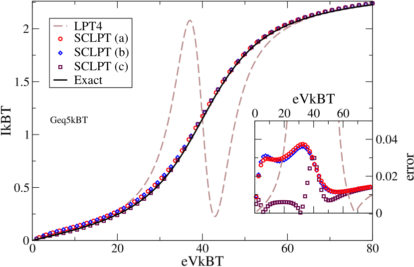
Figure 1: Stationary current $\langle I\rangle$ through the single resonant level as a function of applied bias $eV$ with system-lead coupling $\Gamma_{L}=\Gamma_{R}=5k_{B}T$. The main panel shows the current itself with results plotted for the three SC kernels discussed here, together with the exact solution and the fourth-order LPT results. For this coupling, the LPT solution breaks down when dot level is located around resonance with the chemical potentials. In contrast, all three SC results follow the exact solution closely. The inset shows the absolute value of the difference $\delta I$ between exact and each approximate solution. Further parameters were dot level position $\varepsilon=20k_{B}T$, chemical potentials $\mu_{L}=-\mu_{R}=eV/2$, and cut-off $X_{C}=300k_{B}T$.

In Fig. 1 we show the current calculated with our three SC kernels alongside the exact result and that from straightforward fourth-order LPT. Results are shown for a system-lead coupling of $\Gamma_{R}=\Gamma_{L}=5k_{B}T$. As is clear, at this coupling the fourth-order perturbative expansion LPT solution breaks down badly when the dot level is located around resonance with the chemical potentials. This is in line with the finding of Refs.thi05 ; ce09 , which found the fourth-order ME calculation to be reliable across the full bias range for a coupling $\Gamma_{R}/k_{B}T\lesssim 1/2$. In contrast, all three SC kernels give a very good account of the current. Scrutiny of the inset, which shows the difference between exact an approximate solutions, shows that $\Sigma^{(c)}$ is the most accurate across the bias range, and that $\Sigma^{(a)}$ gives comparable results to the other kernels despite being much easier to calculate.

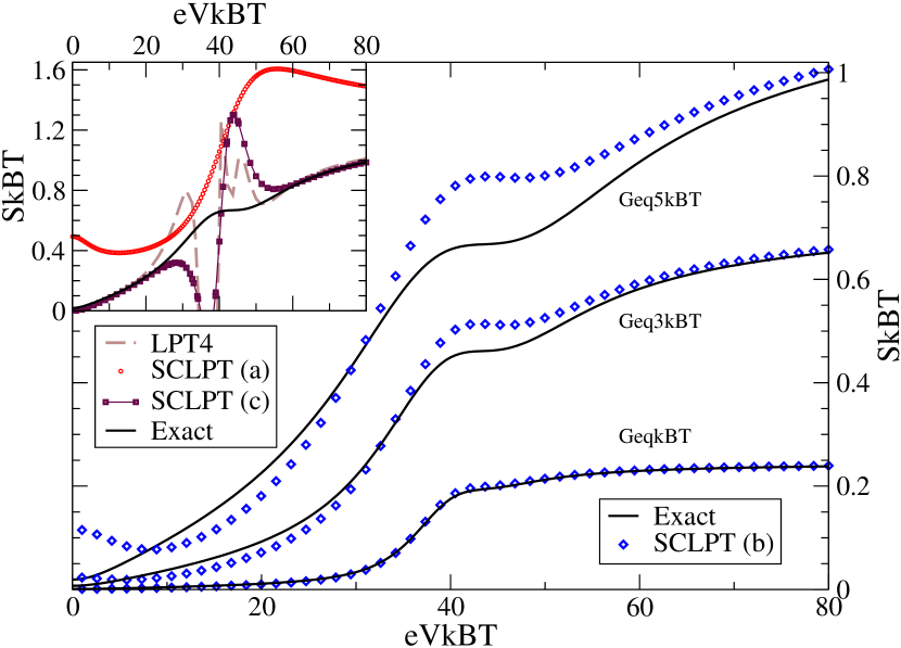
Figure 2: Zero-frequency shotnoise $S$ for the single resonant level as a function of bias. The main panel shows a comparison of the results from the self-consistent $\Sigma^{(b)}$ scheme with the exact results for three different couplings: $\Gamma_{R}=\Gamma_{L}=1,3,5~{}k_{B}T$. The inset shows results for fourth-order LPT and the other two SC kernels for a coupling of $\Gamma_{R}=\Gamma_{L}=5k_{B}T$. Other parameters as in Fig. 1.

Figure 2 shows results for the shotnoise of this model. Starting with the inset we see that that the LPT4 results once again break down around resonance. Moreover, we see that neither $\Sigma^{(a)}$ nor $\Sigma^{(c)}$ provides a good description across the whole bias range. The results for $\Sigma^{(c)}$ break down around resonce in a fashion similar to the LPT solution and this can be attributed to the inclusion of unbroadened propagators in the kernel. Results at large and small bias for this kernel are nevertheless very good. Results for kernel $\Sigma^{(a)}$ break down in a different manner; there is no abrupt behaviour around resonance, but the predicted value of the shotnoise is everywhere much higher than the exact solution. This difference is significant and remains even when the coupling is reduced. This error can be traced to the failure to includes diagrams with crossings. In particular, at fourth order, direct and exchange contributions are of similar magnitude, but with opposite sign. Failure to include diagrams with crossings therefore leads a large portion of the direct contribution remaining uncancelled, and this leads to the overestimated shotnoise. This problem is not manifest in the current because, for this model at least, the fourth-order exchange term does not contribute anyway. We must therefore conclude that this SCBorn-type kernel is unreliable for calculating shotnoise, and by extension higher counting statistics in this intermediate coupling regime.

The main panel shows results for kernel $\Sigma^{(b)}$ and we see that this kernel does give a good account of the shotnoise across the bias range. For higher couplings, the SC results remain qualitatively correct except at low bias, when the system is in the cotunneling regime. Here the SC solution shows a spurious increase of the the shotnoise with decreasing bias. This arises from the conflict of requiring both that the sequential contribution vanish in this cotunneling limit, but also be finite to generate the correct direct cotunneling diagram under iteration. Clearly these two requirements can not be met at the same time, and this leads to a loss of accuracy in this regime.

VII Conclusions

In this paper we have described a method for calculating counting statistics using self-consistent kernels. Three different SC kernels were introduced and we have considered current and shotnoise for the single resonant level as an example application. For this model, all three kernels provide good results for the current, significantly better than could be achieved with straightforward perturbative techniques. On the other hand, only $\Sigma^{(b)}$ is able to provide good results for the shotnoise, in particular when the dot level is around resonance with the chemical potentials. This is the most interesting regime since simple LPT performs well at both high bias and in the cotunneling regime.

Although the above comparison is made for a non-interacting model, we expect the conclusions to hold broadly true for interacting models in the intermediate coupling regime considered here. It remains as future work to see how these SC techniques perform in strongly-coupled interacting systems in which genuine nonperturbative effects, such as the Kondo resonance kondotheory ; kondoexp , come into play.

Appendix A Diagrams

Although we will leave much of the detail of the LPT expansion to I, it behoves us here to discuss those elements relevant to the translation of our diagrams into the corresponding analytic LPT expressions. The (nonSC-) LPT sequential diagram of Eq. (6) reads

$$\Sigma^{(2)}(z) = \mathchoice{\vbox{\hbox to0.0pt{\kern 0.0pt\kern 3.93124pt\hbox{\vrule width=0.50003pt,height=0.0pt,depth=4.30554pt\vrule width=18.50829pt,height=0.0pt,depth=0.50003pt\vrule width=0.50003pt,height=0.0pt,depth=4.30554pt}\hss}\vskip 2.15277pt\vskip 6.83331pt}}{\vbox{\hbox to0.0pt{\kern 0.0pt\kern 3.93124pt\hbox{\vrule width=0.50003pt,height=0.0pt,depth=4.30554pt\vrule width=18.50829pt,height=0.0pt,depth=0.50003pt\vrule width=0.50003pt,height=0.0pt,depth=4.30554pt}\hss}\vskip 2.15277pt\vskip 6.83331pt}}{\vbox{\hbox to0.0pt{\kern 0.0pt\kern 2.75186pt\hbox{\vrule width=0.50003pt,height=0.0pt,depth=4.30554pt\vrule width=11.40027pt,height=0.0pt,depth=0.50003pt\vrule width=0.50003pt,height=0.0pt,depth=4.30554pt}\hss}\vskip 2.15277pt\vskip 4.78333pt}}{\vbox{\hbox to0.0pt{\kern 0.0pt\kern 1.96562pt\hbox{\vrule width=0.50003pt,height=0.0pt,depth=4.30554pt\vrule width=8.14304pt,height=0.0pt,depth=0.50003pt\vrule width=0.50003pt,height=0.0pt,depth=4.30554pt}\hss}\vskip 2.15277pt\vskip 3.41666pt}}G\underset{z}{-}G,$$ (37)

and this translates as

$$\Sigma^{(2)}(z) = (-1)G^{p_{2}}_{2}\Omega_{\mathrm{S}}(z_{1})G^{p_{1}}_{1}\gamma_{21}^{p_{2}p_{1}}.$$ (38)

Similarly, the fourth-order exchange term has the diagram

$$\Sigma^{(4X)}(z) = \mathchoice{\vbox{\hbox to0.0pt{\kern 0.0pt\kern 3.93124pt\hbox{\vrule width=0.50003pt,height=0.0pt,depth=4.30554pt\vrule width=37.01657pt,height=0.0pt,depth=0.50003pt\vrule width=0.50003pt,height=0.0pt,depth=4.30554pt}\hss}\vskip 2.15277pt\vskip 6.83331pt}}{\vbox{\hbox to0.0pt{\kern 0.0pt\kern 3.93124pt\hbox{\vrule width=0.50003pt,height=0.0pt,depth=4.30554pt\vrule width=37.01657pt,height=0.0pt,depth=0.50003pt\vrule width=0.50003pt,height=0.0pt,depth=4.30554pt}\hss}\vskip 2.15277pt\vskip 6.83331pt}}{\vbox{\hbox to0.0pt{\kern 0.0pt\kern 2.75186pt\hbox{\vrule width=0.50003pt,height=0.0pt,depth=4.30554pt\vrule width=22.80054pt,height=0.0pt,depth=0.50003pt\vrule width=0.50003pt,height=0.0pt,depth=4.30554pt}\hss}\vskip 2.15277pt\vskip 4.78333pt}}{\vbox{\hbox to0.0pt{\kern 0.0pt\kern 1.96562pt\hbox{\vrule width=0.50003pt,height=0.0pt,depth=4.30554pt\vrule width=16.28607pt,height=0.0pt,depth=0.50003pt\vrule width=0.50003pt,height=0.0pt,depth=4.30554pt}\hss}\vskip 2.15277pt\vskip 3.41666pt}}\mathchoice{\vbox{\hbox to0.0pt{\kern 18.50829pt\kern 3.93124pt\hbox{\vrule width=0.50003pt,height=0.0pt,depth=8.61108pt\vrule width=37.01657pt,height=0.0pt,depth=0.50003pt\vrule width=0.50003pt,height=0.0pt,depth=8.61108pt}\hss}\vskip 2.15277pt\vskip 6.83331pt}}{\vbox{\hbox to0.0pt{\kern 18.50829pt\kern 3.93124pt\hbox{\vrule width=0.50003pt,height=0.0pt,depth=8.61108pt\vrule width=37.01657pt,height=0.0pt,depth=0.50003pt\vrule width=0.50003pt,height=0.0pt,depth=8.61108pt}\hss}\vskip 2.15277pt\vskip 6.83331pt}}{\vbox{\hbox to0.0pt{\kern 11.40027pt\kern 2.75186pt\hbox{\vrule width=0.50003pt,height=0.0pt,depth=8.61108pt\vrule width=22.80054pt,height=0.0pt,depth=0.50003pt\vrule width=0.50003pt,height=0.0pt,depth=8.61108pt}\hss}\vskip 2.15277pt\vskip 4.78333pt}}{\vbox{\hbox to0.0pt{\kern 8.14304pt\kern 1.96562pt\hbox{\vrule width=0.50003pt,height=0.0pt,depth=8.61108pt\vrule width=16.28607pt,height=0.0pt,depth=0.50003pt\vrule width=0.50003pt,height=0.0pt,depth=8.61108pt}\hss}\vskip 2.15277pt\vskip 3.41666pt}}G\underset{z}{-}G\underset{z}{-}G\underset{z}{-}G,$$ (39)

which translates as

$$\Sigma^{(4X)}(z) = (-1)G^{p_{4}}_{4}\Omega_{\mathrm{S}}(z_{3})G^{p_{3}}_{3}\Omega_{\mathrm{S}}(z_{2})$$ (40)

$$~{}~{}~{}\times G^{p_{2}}_{2}\Omega_{\mathrm{S}}(z_{1})G^{p_{1}}_{1}\gamma_{42}^{p_{4}p_{2}}\gamma_{31}^{p_{3}p_{1}}.$$

In these expressions $G^{p}_{1}$ are Liouville-space tunnel vertices which add or remove electrons from the system, with multi-index subscript ‘$1$’$=(\xi_{1},k_{1},\alpha_{1})$ denoting direction $\xi=\pm 1$, bath momentum $k_{1}$ and lead ($\alpha=L,R$) indices, and with Keldysh index superscript ($p_{i}=\pm 1$). These diagrams include the free system propagator, which translates as

$$\underset{z}{-}\to\Omega_{\mathrm{S}}(z_{m})=\frac{1}{z_{m}-{\cal L}_{\mathrm{S}}},$$ (41)

with free system Liouvillian ${\cal L}_{\mathrm{S}}$ and with the subscript $m$ determined by the position of the propagator in the diagram. The frequencies $z_{m}$ are given by $z_{m}=z+\sum_{l=m+1}^{n}x_{l}$ with Laplace variable $z$, $n$ the order of the diagram (e.g. $n=2$ for sequential order) and $x_{l}=-i\xi_{l}(\omega_{l}+\mu_{\alpha_{l}})$, with reservoir frequency $\omega_{l}$ and chemical potential $\mu_{\alpha_{l}}$. The reservoir contraction reads

$$\gamma_{21}^{p_{2}p_{1}}=\delta_{2\overline{1}}p_{1}f(-\xi_{1}p_{1}\omega_{1})$$ (42)

with Fermi function $f$, and index notation ‘$\overline{1}$’$=(-\xi_{1},k_{1},\alpha_{1})$. Finally, the sign forefactors in Eq. (38) and Eq. (40) come from a product of $(-i)^{n}$ for the $n$th order diagram and Wick sign $(-1)^{N_{p}}$ with $N_{p}$ the permutation number of the digram (here $N_{p}=0$ for the sequential term and $N_{p}=1$ for the exchange). In all diagrams, summations over all $\xi$, $\alpha$, and $p$, as well as integrations over all bath frequencies, are implied. As in the diagrams of lei08 , one could label each tunnel vertex with appropriates indices, and each propagator with appropriate frequency index. However, since these are given uniquely by position in diagram, there is little advantage in doing so. We will, however, label the propagators with Laplace argument $z$, and/or $\chi$ when appropriate, as our formal manipulations require explicit functions of these variables.

The self-consistent equations of Eqs. (8), (9) and (10) include diagrams as above but with propagator

$$\underset{z}{\eqcirc}\to\frac{1}{z_{m}-{\cal L}_{\mathrm{S}}-\Sigma(z)},$$ (43)

where the self-energy $\Sigma(z)$ is the appropriate one for the calculation in hand, e.g. $\Sigma^{(a)}$, etc.. Moreover, for calculating the counting statistics, the relevant propagators are the $\chi$-dependent ones

$$\underset{\chi;z}{\eqcirc}\to\frac{1}{z_{m}-{\cal L}_{\mathrm{S}}-\Sigma(z;\chi)}.$$ (44)

In discussing $\chi$-dependent quantities, multiplying a diagram by counting-field factor $q(\chi)$, corresponds to multiplication of the corresponding super-operator by the same quantity (under the summation ofcourse). For example, the full $z$ and $\chi$ dependent sequential self-energy diagram of Eq. (14) reads

$$\Sigma^{(a)}(z;\chi) = \mathchoice{\vbox{\hbox to0.0pt{\kern 0.0pt\kern 3.93124pt\hbox{\vrule width=0.50003pt,height=0.0pt,depth=4.30554pt\vrule width=34.20963pt,height=0.0pt,depth=0.50003pt\vrule width=0.50003pt,height=0.0pt,depth=4.30554pt}\hss}\vskip 2.15277pt\vskip 6.83331pt}}{\vbox{\hbox to0.0pt{\kern 0.0pt\kern 3.93124pt\hbox{\vrule width=0.50003pt,height=0.0pt,depth=4.30554pt\vrule width=34.20963pt,height=0.0pt,depth=0.50003pt\vrule width=0.50003pt,height=0.0pt,depth=4.30554pt}\hss}\vskip 2.15277pt\vskip 6.83331pt}}{\vbox{\hbox to0.0pt{\kern 0.0pt\kern 2.75186pt\hbox{\vrule width=0.50003pt,height=0.0pt,depth=4.30554pt\vrule width=20.83568pt,height=0.0pt,depth=0.50003pt\vrule width=0.50003pt,height=0.0pt,depth=4.30554pt}\hss}\vskip 2.15277pt\vskip 4.78333pt}}{\vbox{\hbox to0.0pt{\kern 0.0pt\kern 1.96562pt\hbox{\vrule width=0.50003pt,height=0.0pt,depth=4.30554pt\vrule width=14.88261pt,height=0.0pt,depth=0.50003pt\vrule width=0.50003pt,height=0.0pt,depth=4.30554pt}\hss}\vskip 2.15277pt\vskip 3.41666pt}}G\underset{z;\chi}{\eqcirc}G\;q_{2}(\chi),$$ (45)

and this translates as

$$\Sigma^{(a)}(\chi;z) = G^{p_{2}}_{\bar{1}}\frac{-p_{1}f(-\xi_{1}p_{1}\omega_{1})e^{is_{\alpha_{1}}\xi_{1}\frac{1}{2}\left(p_{1}-p_{2}\right)\chi_{\alpha_{1}}}}{z-x_{1}-{\cal L}_{\mathrm{S}}-\Sigma^{(a)}(z;\chi)}G^{p_{1}}_{1},$$

where we have used the explicit form of $q_{2}(\chi)$ from Eq. (15).

A.1 Kernel expansions

Insight into the approximations provided by our self-consistent kernels can be obtained by expanding the effective propagators

$$\left(\underset{z}{\eqcirc}\right)=\left(\underset{z}{-}\right)+\left(\underset{z}{-}\Sigma(z)\underset{z}{-}\right)+\left(\underset{z}{-}\Sigma(z)\underset{z}{-}\Sigma(z)\underset{z}{-}\right)+\ldots.$$

In this way, we can expand the SC self-energy $\Sigma^{(a)}(z)$ of Eq. (8) as

$$\Sigma^{(a)}(z)=\mathchoice{\vbox{\hbox to0.0pt{\kern 0.0pt\kern 3.93124pt\hbox{\vrule width=0.50003pt,height=0.0pt,depth=4.30554pt\vrule width=32.57906pt,height=0.0pt,depth=0.50003pt\vrule width=0.50003pt,height=0.0pt,depth=4.30554pt}\hss}\vskip 2.15277pt\vskip 6.83331pt}}{\vbox{\hbox to0.0pt{\kern 0.0pt\kern 3.93124pt\hbox{\vrule width=0.50003pt,height=0.0pt,depth=4.30554pt\vrule width=32.57906pt,height=0.0pt,depth=0.50003pt\vrule width=0.50003pt,height=0.0pt,depth=4.30554pt}\hss}\vskip 2.15277pt\vskip 6.83331pt}}{\vbox{\hbox to0.0pt{\kern 0.0pt\kern 2.75186pt\hbox{\vrule width=0.50003pt,height=0.0pt,depth=4.30554pt\vrule width=19.73428pt,height=0.0pt,depth=0.50003pt\vrule width=0.50003pt,height=0.0pt,depth=4.30554pt}\hss}\vskip 2.15277pt\vskip 4.78333pt}}{\vbox{\hbox to0.0pt{\kern 0.0pt\kern 1.96562pt\hbox{\vrule width=0.50003pt,height=0.0pt,depth=4.30554pt\vrule width=14.66733pt,height=0.0pt,depth=0.50003pt\vrule width=0.50003pt,height=0.0pt,depth=4.30554pt}\hss}\vskip 2.15277pt\vskip 3.41666pt}}G\underset{z-x_{1}}{-}G+\mathchoice{\vbox{\hbox to0.0pt{\kern 0.0pt\kern 3.93124pt\hbox{\vrule width=0.50003pt,height=0.0pt,depth=8.61108pt\vrule width=97.73717pt,height=0.0pt,depth=0.50003pt\vrule width=0.50003pt,height=0.0pt,depth=8.61108pt}\hss}\vskip 2.15277pt\vskip 6.83331pt}}{\vbox{\hbox to0.0pt{\kern 0.0pt\kern 3.93124pt\hbox{\vrule width=0.50003pt,height=0.0pt,depth=8.61108pt\vrule width=97.73717pt,height=0.0pt,depth=0.50003pt\vrule width=0.50003pt,height=0.0pt,depth=8.61108pt}\hss}\vskip 2.15277pt\vskip 6.83331pt}}{\vbox{\hbox to0.0pt{\kern 0.0pt\kern 2.75186pt\hbox{\vrule width=0.50003pt,height=0.0pt,depth=8.61108pt\vrule width=59.20285pt,height=0.0pt,depth=0.50003pt\vrule width=0.50003pt,height=0.0pt,depth=8.61108pt}\hss}\vskip 2.15277pt\vskip 4.78333pt}}{\vbox{\hbox to0.0pt{\kern 0.0pt\kern 1.96562pt\hbox{\vrule width=0.50003pt,height=0.0pt,depth=8.61108pt\vrule width=44.00198pt,height=0.0pt,depth=0.50003pt\vrule width=0.50003pt,height=0.0pt,depth=8.61108pt}\hss}\vskip 2.15277pt\vskip 3.41666pt}}\mathchoice{\vbox{\hbox to0.0pt{\kern 32.57906pt\kern 3.93124pt\hbox{\vrule width=0.50003pt,height=0.0pt,depth=4.30554pt\vrule width=32.57906pt,height=0.0pt,depth=0.50003pt\vrule width=0.50003pt,height=0.0pt,depth=4.30554pt}\hss}\vskip 2.15277pt\vskip 6.83331pt}}{\vbox{\hbox to0.0pt{\kern 32.57906pt\kern 3.93124pt\hbox{\vrule width=0.50003pt,height=0.0pt,depth=4.30554pt\vrule width=32.57906pt,height=0.0pt,depth=0.50003pt\vrule width=0.50003pt,height=0.0pt,depth=4.30554pt}\hss}\vskip 2.15277pt\vskip 6.83331pt}}{\vbox{\hbox to0.0pt{\kern 19.73428pt\kern 2.75186pt\hbox{\vrule width=0.50003pt,height=0.0pt,depth=4.30554pt\vrule width=19.73428pt,height=0.0pt,depth=0.50003pt\vrule width=0.50003pt,height=0.0pt,depth=4.30554pt}\hss}\vskip 2.15277pt\vskip 4.78333pt}}{\vbox{\hbox to0.0pt{\kern 14.66733pt\kern 1.96562pt\hbox{\vrule width=0.50003pt,height=0.0pt,depth=4.30554pt\vrule width=14.66733pt,height=0.0pt,depth=0.50003pt\vrule width=0.50003pt,height=0.0pt,depth=4.30554pt}\hss}\vskip 2.15277pt\vskip 3.41666pt}}G\underset{z-x_{1}}{-}G\underset{z-x_{2}}{-}G\underset{z-x_{1}}{-}G+\ldots,$$

where we have made explicit the $x$ variables in the propagators and, in doing so, have taken into account the $\delta$-functions in the bath contractions. The expansion of $\Sigma^{(a)}(z)$ therefore generates a diagram with the same topology as the direct cotunneling term. With $x$-arguments, the exact direct diagram reads

$$\Sigma^{(4D)}(z)=\mathchoice{\vbox{\hbox to0.0pt{\kern 0.0pt\kern 3.93124pt\hbox{\vrule width=0.50003pt,height=0.0pt,depth=8.61108pt\vrule width=111.80794pt,height=0.0pt,depth=0.50003pt\vrule width=0.50003pt,height=0.0pt,depth=8.61108pt}\hss}\vskip 2.15277pt\vskip 6.83331pt}}{\vbox{\hbox to0.0pt{\kern 0.0pt\kern 3.93124pt\hbox{\vrule width=0.50003pt,height=0.0pt,depth=8.61108pt\vrule width=111.80794pt,height=0.0pt,depth=0.50003pt\vrule width=0.50003pt,height=0.0pt,depth=8.61108pt}\hss}\vskip 2.15277pt\vskip 6.83331pt}}{\vbox{\hbox to0.0pt{\kern 0.0pt\kern 2.75186pt\hbox{\vrule width=0.50003pt,height=0.0pt,depth=8.61108pt\vrule width=67.53687pt,height=0.0pt,depth=0.50003pt\vrule width=0.50003pt,height=0.0pt,depth=8.61108pt}\hss}\vskip 2.15277pt\vskip 4.78333pt}}{\vbox{\hbox to0.0pt{\kern 0.0pt\kern 1.96562pt\hbox{\vrule width=0.50003pt,height=0.0pt,depth=8.61108pt\vrule width=50.52628pt,height=0.0pt,depth=0.50003pt\vrule width=0.50003pt,height=0.0pt,depth=8.61108pt}\hss}\vskip 2.15277pt\vskip 3.41666pt}}\mathchoice{\vbox{\hbox to0.0pt{\kern 32.57906pt\kern 3.93124pt\hbox{\vrule width=0.50003pt,height=0.0pt,depth=4.30554pt\vrule width=46.64983pt,height=0.0pt,depth=0.50003pt\vrule width=0.50003pt,height=0.0pt,depth=4.30554pt}\hss}\vskip 2.15277pt\vskip 6.83331pt}}{\vbox{\hbox to0.0pt{\kern 32.57906pt\kern 3.93124pt\hbox{\vrule width=0.50003pt,height=0.0pt,depth=4.30554pt\vrule width=46.64983pt,height=0.0pt,depth=0.50003pt\vrule width=0.50003pt,height=0.0pt,depth=4.30554pt}\hss}\vskip 2.15277pt\vskip 6.83331pt}}{\vbox{\hbox to0.0pt{\kern 19.73428pt\kern 2.75186pt\hbox{\vrule width=0.50003pt,height=0.0pt,depth=4.30554pt\vrule width=28.0683pt,height=0.0pt,depth=0.50003pt\vrule width=0.50003pt,height=0.0pt,depth=4.30554pt}\hss}\vskip 2.15277pt\vskip 4.78333pt}}{\vbox{\hbox to0.0pt{\kern 14.66733pt\kern 1.96562pt\hbox{\vrule width=0.50003pt,height=0.0pt,depth=4.30554pt\vrule width=21.19162pt,height=0.0pt,depth=0.50003pt\vrule width=0.50003pt,height=0.0pt,depth=4.30554pt}\hss}\vskip 2.15277pt\vskip 3.41666pt}}G\underset{z-x_{1}}{-}G\underset{z-x_{1}-x_{2}}{-}G\underset{z-x_{1}}{-}G.$$ (47)

Comparison of Eq. (A.1) and Eq. (47) shows that the fourth-order term in the SC expansion provides an approximation which differs only the $x$ argument of the middle propagator.

Appendix B Matrix representation

In this Liouville-space approach, superoperators such as the Liouvillian can be represented as finite-dimensional matrices and we often make use here of their eigendecomposition. Of particular importance is the decomposition of the $\chi=0$, $z=0$ effective Liouvillian ${\cal W}={\cal W}(0,0^{+})$, from which the stationary properties of the system may be calculated. Since ${\cal W}$ is nonHermitian, it has non-adjoint left, $\langle\!\langle\psi_{a}|$, and right, $|\psi_{a}\rangle\!\rangle$, eigenvectors defined by the equations

$${\cal W}|\psi_{a}\rangle\!\rangle = w_{a}|\psi_{a}\rangle\!\rangle$$

$$\langle\!\langle\psi_{a}|{\cal W} = w_{a}\langle\!\langle\psi_{a}|,$$ (48)

with eigenvalues $w_{a}$ and index $a=0,1,\ldots,N-1$ with $N$ the dimension of ${\cal W}$. Taken together the left and right eigenvectors form a bi-orthonormal set: $\langle\!\langle\psi_{a}|\psi_{a^{\prime}}\rangle\!\rangle=\delta_{a,a^{\prime}}$ and we have the closure relation in Liouvillian space

$$\mathbbm{1}=\sum_{a}|\psi_{a}\rangle\!\rangle\langle\!\langle\psi_{a}|.$$ (49)

The eigendecomposition of the stationary kernel reads

$${\cal W}=\sum_{a}w_{a}|\psi_{a}\rangle\!\rangle\langle\!\langle\psi_{a}|.$$ (50)

Assuming that the system has a unique stationary state, one (and only one) of the eigenvalues will be zero, $w_{0}=0$, and the stationary state itself is given by the corresponding right eigenvector $\rho^{\mathrm{stat}}_{\mathrm{S}}=|\psi_{0}\rangle\!\rangle$. The dual vector $\langle\!\langle\psi_{0}|$ is then the “trace vector” with elements unity at positions mapping to populations and zero at those mapping to coherences. The remaining eigenvalues of ${\cal W}$ have non-positive real parts and, if complex, occur in complex conjugate pairs.

Appendix C Integrals

We now discuss the analytic evaluation of the integrals required here. For convenience we set $k_{B}T=1$. The $z=0$ integral equation for $\Sigma^{(a)}(z=0)$ reads

$$\Sigma^{(a)}(0) = \int d\omega_{1}G^{p_{2}}_{\bar{1}}\frac{-p_{1}f(-\xi_{1}p_{1}\omega_{1})}{0^{+}+i\xi_{1}(\omega_{1}+\mu_{\alpha_{1}})-{\cal W}^{(a)}(0)}G^{p_{1}}_{1}.$$

Using the eigendecomposition for ${\cal W}^{(a)}(0)$, as in Eq. (50), we write this as

$$\Sigma^{(a)}(0) = -p_{1}G^{p_{2}}_{\bar{1}}|\psi_{a}\rangle\!\rangle\langle\!\langle\psi_{a}|G^{p_{1}}_{1}$$

$$\times\int d\omega_{1}\frac{f(-\xi_{1}p_{1}\omega_{1})}{0^{+}+i\xi_{1}(\omega_{1}+\mu_{\alpha_{1}})-w_{a}}$$

$$= -2\pi p_{1}G^{p_{2}}_{\bar{1}}|\psi_{a}\rangle\!\rangle\langle\!\langle\psi_{a}|G^{p_{1}}_{1}~{}I^{(2)}_{p_{1}}(\xi_{1}\mu_{\alpha_{1}}+iw_{a}),$$

which defines the sequential integral, $I_{p}^{(2)}(\lambda)$. This integral can be evaluated as in I with the introduction of a Lorentzian cut-off function ${\cal D}(\omega)=X_{C}^{2}/\left\{(\omega-\omega_{0})^{2}+X_{C}^{2}\right\}$, with band-centre $\omega_{0}$ chosen for convenience, as

$$I_{p}^{(2)}(\lambda)\equiv\frac{i}{2\pi}\int d\omega\frac{f(\omega)}{i0^{+}+p\omega-\lambda} = \frac{1}{2}f(p\lambda)+\frac{ip}{2\pi}\phi(\lambda).$$

Here $\phi(\omega)=\frac{1}{2}\left(\frac{}{}g(\omega)+g(-\omega)-g(\omega+iX_{c})-g(-\omega+iX_{c})\right)$, with $g(\omega)\equiv\Psi\left(\frac{1}{2}+\frac{\omega}{2\pi iT}\right)$, and $\Psi$ the digamma function.

As discussed in I, evaluation of fourth-order terms requires the integral

$$I^{p_{1}p_{2}}(\lambda_{2},\lambda_{3}) = \int d\omega_{1}d\omega_{2}\frac{f(p_{1}\omega_{1})f(p_{2}\omega_{2})}{(i0^{+}+\omega_{1}+\omega_{2}-\lambda_{2})(i0^{+}+\omega_{1}-\lambda_{3})}.$$ (51)

In straightforward Liouvillian Perturbation theory, the $\lambda_{i}$ are real; for self-consistent calculations, they can be complex and this means that we need the result for this integral in a slightly more general form than given in I. We have

$$I^{p_{1}p_{2}}(\lambda_{2},\lambda_{3}) = p_{1}p_{2}G(\lambda_{2},\lambda_{3})+p_{1}\widetilde{G}(\lambda_{3})+p_{1}p_{2}H(\lambda_{2},\lambda_{3})+\mathrm{const}$$ (52)

with “const” an unimportant constant. The first two part functions are

$$G(\lambda_{2},\lambda_{3}) = 2\pi^{2}(\textstyle{\frac{1}{2}}+b(\lambda_{2}))\left\{I^{(2)}_{+1}(\lambda_{3})-I^{(2)}_{+1}(\lambda_{32})\right\}+g(-\lambda_{3})\phi(\lambda_{32})$$ (53)

$$-\textstyle{\frac{1}{2}}g(-\lambda_{3}+iX_{C})\phi(\lambda_{32}-iX_{C})-\textstyle{\frac{1}{2}}g(\lambda_{3}+iX_{C})\phi(\lambda_{32}+iX_{C}),$$

and

$$\widetilde{G}(\lambda_{3})=-\pi^{2}I^{(2)}_{+1}(\lambda_{3}),$$ (54)

with $\lambda_{ij}=\lambda_{i}-\lambda_{j}$ and Bose-Einstein distribution function $b(x)=\left(e^{x}-1\right)^{-1}$. The third contribution is more complicated and reads

$$H(\lambda_{2},\lambda_{3}) = \sum_{k=1,3,5,\ldots}^{\infty}g(-\lambda_{2}+i\pi k)\left\{\frac{1}{\lambda_{32}-iX_{C}+i\pi k}+\frac{1}{\lambda_{32}+iX_{C}+i\pi k}-\frac{2}{\lambda_{32}+i\pi k}\right\}$$ (55)

$$~{}~{}~{}~{}~{}~{}-g(-\lambda_{2}+iX_{C}+i\pi k)\left\{\frac{1}{\lambda_{32}+i\pi k}+\frac{1}{\lambda_{32}+2iX_{C}+i\pi k}-\frac{2}{\lambda_{32}+iX_{C}+i\pi k}\right\}$$

$$~{}~{}~{}~{}~{}~{}+g(\lambda_{2}+i\pi k)\left\{\frac{1}{-\lambda_{32}-iX_{C}+i\pi k}+\frac{1}{-\lambda_{32}+iX_{C}+i\pi k}-\frac{2}{-\lambda_{32}+i\pi k}\right\}$$

$$~{}~{}~{}~{}~{}~{}-g(\lambda_{2}+iX_{C}+i\pi k)\left\{\frac{1}{-\lambda_{32}+i\pi k}+\frac{1}{-\lambda_{32}+2iX_{C}+i\pi k}-\frac{2}{-\lambda_{32}+iX_{C}+i\pi k}\right\}.$$

It remains to discuss the translation and integration of diagrams of the form $\mathchoice{\vbox{\hbox to0.0pt{\kern 0.0pt\kern 3.93124pt\hbox{\vrule width=0.50003pt,height=0.0pt,depth=4.30554pt\vrule width=39.76517pt,height=0.0pt,depth=0.50003pt\vrule width=0.50003pt,height=0.0pt,depth=4.30554pt}\hss}\vskip 2.15277pt\vskip 6.83331pt}}{\vbox{\hbox to0.0pt{\kern 0.0pt\kern 3.93124pt\hbox{\vrule width=0.50003pt,height=0.0pt,depth=4.30554pt\vrule width=39.76517pt,height=0.0pt,depth=0.50003pt\vrule width=0.50003pt,height=0.0pt,depth=4.30554pt}\hss}\vskip 2.15277pt\vskip 6.83331pt}}{\vbox{\hbox to0.0pt{\kern 0.0pt\kern 2.75186pt\hbox{\vrule width=0.50003pt,height=0.0pt,depth=4.30554pt\vrule width=29.50223pt,height=0.0pt,depth=0.50003pt\vrule width=0.50003pt,height=0.0pt,depth=4.30554pt}\hss}\vskip 2.15277pt\vskip 4.78333pt}}{\vbox{\hbox to0.0pt{\kern 0.0pt\kern 1.96562pt\hbox{\vrule width=0.50003pt,height=0.0pt,depth=4.30554pt\vrule width=22.66028pt,height=0.0pt,depth=0.50003pt\vrule width=0.50003pt,height=0.0pt,depth=4.30554pt}\hss}\vskip 2.15277pt\vskip 3.41666pt}}G\eqcirc M\eqcirc G$, such as occur in Eq. (23) for example. The analytic expression of this diagram reads

$$-p_{1}\int d\omega_{1}G^{p_{2}}_{\bar{1}}\frac{1}{0^{+}+i\xi_{1}(\omega_{1}+\mu_{\alpha_{1}})-{\cal W}^{(a)}(0)}M\frac{1}{0^{+}+i\xi_{1}(\omega_{1}+\mu_{\alpha_{1}})-{\cal W}^{(a)}(0)}G^{p_{1}}_{1}f(-\xi_{1}p_{1}\omega_{1})$$ (56)

Introduction of the eigendecomposition for the stationary kernels and the employ of a partial fraction decomposition allows us to write this as

$$-p_{1}G^{p_{2}}_{\bar{1}}|\psi_{a}\rangle\!\rangle\langle\!\langle\psi_{a}|M|\psi_{a^{\prime}}\rangle\!\rangle\langle\!\langle\psi_{a^{\prime}}|G^{p_{1}}_{1}~{}\int d\omega_{1}\frac{f(-\xi_{1}p_{1}\omega_{1})}{w_{a}-w_{a^{\prime}}}\left(\frac{1}{0^{+}+i\xi_{1}(\omega_{1}+\mu_{\alpha_{1}})-w_{a}}-\frac{1}{0^{+}+i\xi_{1}(\omega_{1}+\mu_{\alpha_{1}})-w_{a^{\prime}}}\right)$$

Identifying the sequential integrals, this becomes

$$-2\pi p_{1}G^{p_{2}}_{\bar{1}}|\psi_{a}\rangle\!\rangle\langle\!\langle\psi_{a}|M|\psi_{a^{\prime}}\rangle\!\rangle\langle\!\langle\psi_{a^{\prime}}|G^{p_{1}}_{1}~{}\frac{I^{(2)}_{p_{1}}(\mu_{\alpha_{1}}+iw_{a})-I^{(2)}_{p_{1}}(\mu_{\alpha_{1}}+iw_{a^{\prime}})}{w_{a}-w_{a^{\prime}}}.$$ (57)

In the case that $w_{a}=w_{a^{\prime}}$, the differential quotient is recognised and the integral part replaced with $d/dw_{a}I^{(2)}_{p_{1}}(\mu_{\alpha_{1}}+iw_{a})$. The evaluation of similar cotunneling-type terms follows analogously.

Appendix D Jump-operator equations for the $\Sigma^{(b)}$ SC kernel

The four equations corresponding to Eqs (23-26) for the current blocks of $\Sigma^{(b)}$ are:

$${\cal J}^{\prime} = \mathchoice{\vbox{\hbox to0.0pt{\kern 0.0pt\kern 3.93124pt\hbox{\vrule width=0.50003pt,height=0.0pt,depth=4.30554pt\vrule width=15.64029pt,height=0.0pt,depth=0.50003pt\vrule width=0.50003pt,height=0.0pt,depth=4.30554pt}\hss}\vskip 2.15277pt\vskip 6.83331pt}}{\vbox{\hbox to0.0pt{\kern 0.0pt\kern 3.93124pt\hbox{\vrule width=0.50003pt,height=0.0pt,depth=4.30554pt\vrule width=15.64029pt,height=0.0pt,depth=0.50003pt\vrule width=0.50003pt,height=0.0pt,depth=4.30554pt}\hss}\vskip 2.15277pt\vskip 6.83331pt}}{\vbox{\hbox to0.0pt{\kern 0.0pt\kern 2.75186pt\hbox{\vrule width=0.50003pt,height=0.0pt,depth=4.30554pt\vrule width=10.9482pt,height=0.0pt,depth=0.50003pt\vrule width=0.50003pt,height=0.0pt,depth=4.30554pt}\hss}\vskip 2.15277pt\vskip 4.78333pt}}{\vbox{\hbox to0.0pt{\kern 0.0pt\kern 1.96562pt\hbox{\vrule width=0.50003pt,height=0.0pt,depth=4.30554pt\vrule width=7.82014pt,height=0.0pt,depth=0.50003pt\vrule width=0.50003pt,height=0.0pt,depth=4.30554pt}\hss}\vskip 2.15277pt\vskip 3.41666pt}}G\eqcirc G~{}q_{2}^{\prime}+\mathchoice{\vbox{\hbox to0.0pt{\kern 0.0pt\kern 3.93124pt\hbox{\vrule width=0.50003pt,height=0.0pt,depth=4.30554pt\vrule width=36.836pt,height=0.0pt,depth=0.50003pt\vrule width=0.50003pt,height=0.0pt,depth=4.30554pt}\hss}\vskip 2.15277pt\vskip 6.83331pt}}{\vbox{\hbox to0.0pt{\kern 0.0pt\kern 3.93124pt\hbox{\vrule width=0.50003pt,height=0.0pt,depth=4.30554pt\vrule width=36.836pt,height=0.0pt,depth=0.50003pt\vrule width=0.50003pt,height=0.0pt,depth=4.30554pt}\hss}\vskip 2.15277pt\vskip 6.83331pt}}{\vbox{\hbox to0.0pt{\kern 0.0pt\kern 2.75186pt\hbox{\vrule width=0.50003pt,height=0.0pt,depth=4.30554pt\vrule width=27.45181pt,height=0.0pt,depth=0.50003pt\vrule width=0.50003pt,height=0.0pt,depth=4.30554pt}\hss}\vskip 2.15277pt\vskip 4.78333pt}}{\vbox{\hbox to0.0pt{\kern 0.0pt\kern 1.96562pt\hbox{\vrule width=0.50003pt,height=0.0pt,depth=4.30554pt\vrule width=21.19571pt,height=0.0pt,depth=0.50003pt\vrule width=0.50003pt,height=0.0pt,depth=4.30554pt}\hss}\vskip 2.15277pt\vskip 3.41666pt}}\mathchoice{\vbox{\hbox to0.0pt{\kern 15.64029pt\kern 3.93124pt\hbox{\vrule width=0.50003pt,height=0.0pt,depth=8.61108pt\vrule width=36.836pt,height=0.0pt,depth=0.50003pt\vrule width=0.50003pt,height=0.0pt,depth=8.61108pt}\hss}\vskip 2.15277pt\vskip 6.83331pt}}{\vbox{\hbox to0.0pt{\kern 15.64029pt\kern 3.93124pt\hbox{\vrule width=0.50003pt,height=0.0pt,depth=8.61108pt\vrule width=36.836pt,height=0.0pt,depth=0.50003pt\vrule width=0.50003pt,height=0.0pt,depth=8.61108pt}\hss}\vskip 2.15277pt\vskip 6.83331pt}}{\vbox{\hbox to0.0pt{\kern 10.9482pt\kern 2.75186pt\hbox{\vrule width=0.50003pt,height=0.0pt,depth=8.61108pt\vrule width=27.45181pt,height=0.0pt,depth=0.50003pt\vrule width=0.50003pt,height=0.0pt,depth=8.61108pt}\hss}\vskip 2.15277pt\vskip 4.78333pt}}{\vbox{\hbox to0.0pt{\kern 7.82014pt\kern 1.96562pt\hbox{\vrule width=0.50003pt,height=0.0pt,depth=8.61108pt\vrule width=21.19571pt,height=0.0pt,depth=0.50003pt\vrule width=0.50003pt,height=0.0pt,depth=8.61108pt}\hss}\vskip 2.15277pt\vskip 3.41666pt}}G\eqcirc G\eqcirc G\eqcirc G~{}q_{4X}^{\prime}+\mathchoice{\vbox{\hbox to0.0pt{\kern 0.0pt\kern 3.93124pt\hbox{\vrule width=0.50003pt,height=0.0pt,depth=4.30554pt\vrule width=30.09698pt,height=0.0pt,depth=0.50003pt\vrule width=0.50003pt,height=0.0pt,depth=4.30554pt}\hss}\vskip 2.15277pt\vskip 6.83331pt}}{\vbox{\hbox to0.0pt{\kern 0.0pt\kern 3.93124pt\hbox{\vrule width=0.50003pt,height=0.0pt,depth=4.30554pt\vrule width=30.09698pt,height=0.0pt,depth=0.50003pt\vrule width=0.50003pt,height=0.0pt,depth=4.30554pt}\hss}\vskip 2.15277pt\vskip 6.83331pt}}{\vbox{\hbox to0.0pt{\kern 0.0pt\kern 2.75186pt\hbox{\vrule width=0.50003pt,height=0.0pt,depth=4.30554pt\vrule width=21.08987pt,height=0.0pt,depth=0.50003pt\vrule width=0.50003pt,height=0.0pt,depth=4.30554pt}\hss}\vskip 2.15277pt\vskip 4.78333pt}}{\vbox{\hbox to0.0pt{\kern 0.0pt\kern 1.96562pt\hbox{\vrule width=0.50003pt,height=0.0pt,depth=4.30554pt\vrule width=15.37848pt,height=0.0pt,depth=0.50003pt\vrule width=0.50003pt,height=0.0pt,depth=4.30554pt}\hss}\vskip 2.15277pt\vskip 3.41666pt}}G\eqcirc{\cal J}^{\prime}\eqcirc G+\mathchoice{\vbox{\hbox to0.0pt{\kern 0.0pt\kern 3.93124pt\hbox{\vrule width=0.50003pt,height=0.0pt,depth=4.30554pt\vrule width=51.2927pt,height=0.0pt,depth=0.50003pt\vrule width=0.50003pt,height=0.0pt,depth=4.30554pt}\hss}\vskip 2.15277pt\vskip 6.83331pt}}{\vbox{\hbox to0.0pt{\kern 0.0pt\kern 3.93124pt\hbox{\vrule width=0.50003pt,height=0.0pt,depth=4.30554pt\vrule width=51.2927pt,height=0.0pt,depth=0.50003pt\vrule width=0.50003pt,height=0.0pt,depth=4.30554pt}\hss}\vskip 2.15277pt\vskip 6.83331pt}}{\vbox{\hbox to0.0pt{\kern 0.0pt\kern 2.75186pt\hbox{\vrule width=0.50003pt,height=0.0pt,depth=4.30554pt\vrule width=37.59349pt,height=0.0pt,depth=0.50003pt\vrule width=0.50003pt,height=0.0pt,depth=4.30554pt}\hss}\vskip 2.15277pt\vskip 4.78333pt}}{\vbox{\hbox to0.0pt{\kern 0.0pt\kern 1.96562pt\hbox{\vrule width=0.50003pt,height=0.0pt,depth=4.30554pt\vrule width=28.75404pt,height=0.0pt,depth=0.50003pt\vrule width=0.50003pt,height=0.0pt,depth=4.30554pt}\hss}\vskip 2.15277pt\vskip 3.41666pt}}\mathchoice{\vbox{\hbox to0.0pt{\kern 32.8747pt\kern 3.93124pt\hbox{\vrule width=0.50003pt,height=0.0pt,depth=8.61108pt\vrule width=36.836pt,height=0.0pt,depth=0.50003pt\vrule width=0.50003pt,height=0.0pt,depth=8.61108pt}\hss}\vskip 2.15277pt\vskip 6.83331pt}}{\vbox{\hbox to0.0pt{\kern 32.8747pt\kern 3.93124pt\hbox{\vrule width=0.50003pt,height=0.0pt,depth=8.61108pt\vrule width=36.836pt,height=0.0pt,depth=0.50003pt\vrule width=0.50003pt,height=0.0pt,depth=8.61108pt}\hss}\vskip 2.15277pt\vskip 6.83331pt}}{\vbox{\hbox to0.0pt{\kern 23.86758pt\kern 2.75186pt\hbox{\vrule width=0.50003pt,height=0.0pt,depth=8.61108pt\vrule width=27.45181pt,height=0.0pt,depth=0.50003pt\vrule width=0.50003pt,height=0.0pt,depth=8.61108pt}\hss}\vskip 2.15277pt\vskip 4.78333pt}}{\vbox{\hbox to0.0pt{\kern 18.15619pt\kern 1.96562pt\hbox{\vrule width=0.50003pt,height=0.0pt,depth=8.61108pt\vrule width=21.19571pt,height=0.0pt,depth=0.50003pt\vrule width=0.50003pt,height=0.0pt,depth=8.61108pt}\hss}\vskip 2.15277pt\vskip 3.41666pt}}G\eqcirc{\cal J}^{\prime}\eqcirc G\eqcirc G\eqcirc G$$ (58)

$$+~{}\mathchoice{\vbox{\hbox to0.0pt{\kern 0.0pt\kern 3.93124pt\hbox{\vrule width=0.50003pt,height=0.0pt,depth=4.30554pt\vrule width=51.2927pt,height=0.0pt,depth=0.50003pt\vrule width=0.50003pt,height=0.0pt,depth=4.30554pt}\hss}\vskip 2.15277pt\vskip 6.83331pt}}{\vbox{\hbox to0.0pt{\kern 0.0pt\kern 3.93124pt\hbox{\vrule width=0.50003pt,height=0.0pt,depth=4.30554pt\vrule width=51.2927pt,height=0.0pt,depth=0.50003pt\vrule width=0.50003pt,height=0.0pt,depth=4.30554pt}\hss}\vskip 2.15277pt\vskip 6.83331pt}}{\vbox{\hbox to0.0pt{\kern 0.0pt\kern 2.75186pt\hbox{\vrule width=0.50003pt,height=0.0pt,depth=4.30554pt\vrule width=37.59349pt,height=0.0pt,depth=0.50003pt\vrule width=0.50003pt,height=0.0pt,depth=4.30554pt}\hss}\vskip 2.15277pt\vskip 4.78333pt}}{\vbox{\hbox to0.0pt{\kern 0.0pt\kern 1.96562pt\hbox{\vrule width=0.50003pt,height=0.0pt,depth=4.30554pt\vrule width=28.75404pt,height=0.0pt,depth=0.50003pt\vrule width=0.50003pt,height=0.0pt,depth=4.30554pt}\hss}\vskip 2.15277pt\vskip 3.41666pt}}\mathchoice{\vbox{\hbox to0.0pt{\kern 18.418pt\kern 3.93124pt\hbox{\vrule width=0.50003pt,height=0.0pt,depth=8.61108pt\vrule width=51.2927pt,height=0.0pt,depth=0.50003pt\vrule width=0.50003pt,height=0.0pt,depth=8.61108pt}\hss}\vskip 2.15277pt\vskip 6.83331pt}}{\vbox{\hbox to0.0pt{\kern 18.418pt\kern 3.93124pt\hbox{\vrule width=0.50003pt,height=0.0pt,depth=8.61108pt\vrule width=51.2927pt,height=0.0pt,depth=0.50003pt\vrule width=0.50003pt,height=0.0pt,depth=8.61108pt}\hss}\vskip 2.15277pt\vskip 6.83331pt}}{\vbox{\hbox to0.0pt{\kern 13.7259pt\kern 2.75186pt\hbox{\vrule width=0.50003pt,height=0.0pt,depth=8.61108pt\vrule width=37.59349pt,height=0.0pt,depth=0.50003pt\vrule width=0.50003pt,height=0.0pt,depth=8.61108pt}\hss}\vskip 2.15277pt\vskip 4.78333pt}}{\vbox{\hbox to0.0pt{\kern 10.59785pt\kern 1.96562pt\hbox{\vrule width=0.50003pt,height=0.0pt,depth=8.61108pt\vrule width=28.75404pt,height=0.0pt,depth=0.50003pt\vrule width=0.50003pt,height=0.0pt,depth=8.61108pt}\hss}\vskip 2.15277pt\vskip 3.41666pt}}G\eqcirc G\eqcirc{\cal J}^{\prime}\eqcirc G\eqcirc G+\mathchoice{\vbox{\hbox to0.0pt{\kern 0.0pt\kern 3.93124pt\hbox{\vrule width=0.50003pt,height=0.0pt,depth=4.30554pt\vrule width=36.836pt,height=0.0pt,depth=0.50003pt\vrule width=0.50003pt,height=0.0pt,depth=4.30554pt}\hss}\vskip 2.15277pt\vskip 6.83331pt}}{\vbox{\hbox to0.0pt{\kern 0.0pt\kern 3.93124pt\hbox{\vrule width=0.50003pt,height=0.0pt,depth=4.30554pt\vrule width=36.836pt,height=0.0pt,depth=0.50003pt\vrule width=0.50003pt,height=0.0pt,depth=4.30554pt}\hss}\vskip 2.15277pt\vskip 6.83331pt}}{\vbox{\hbox to0.0pt{\kern 0.0pt\kern 2.75186pt\hbox{\vrule width=0.50003pt,height=0.0pt,depth=4.30554pt\vrule width=27.45181pt,height=0.0pt,depth=0.50003pt\vrule width=0.50003pt,height=0.0pt,depth=4.30554pt}\hss}\vskip 2.15277pt\vskip 4.78333pt}}{\vbox{\hbox to0.0pt{\kern 0.0pt\kern 1.96562pt\hbox{\vrule width=0.50003pt,height=0.0pt,depth=4.30554pt\vrule width=21.19571pt,height=0.0pt,depth=0.50003pt\vrule width=0.50003pt,height=0.0pt,depth=4.30554pt}\hss}\vskip 2.15277pt\vskip 3.41666pt}}\mathchoice{\vbox{\hbox to0.0pt{\kern 18.418pt\kern 3.93124pt\hbox{\vrule width=0.50003pt,height=0.0pt,depth=8.61108pt\vrule width=51.2927pt,height=0.0pt,depth=0.50003pt\vrule width=0.50003pt,height=0.0pt,depth=8.61108pt}\hss}\vskip 2.15277pt\vskip 6.83331pt}}{\vbox{\hbox to0.0pt{\kern 18.418pt\kern 3.93124pt\hbox{\vrule width=0.50003pt,height=0.0pt,depth=8.61108pt\vrule width=51.2927pt,height=0.0pt,depth=0.50003pt\vrule width=0.50003pt,height=0.0pt,depth=8.61108pt}\hss}\vskip 2.15277pt\vskip 6.83331pt}}{\vbox{\hbox to0.0pt{\kern 13.7259pt\kern 2.75186pt\hbox{\vrule width=0.50003pt,height=0.0pt,depth=8.61108pt\vrule width=37.59349pt,height=0.0pt,depth=0.50003pt\vrule width=0.50003pt,height=0.0pt,depth=8.61108pt}\hss}\vskip 2.15277pt\vskip 4.78333pt}}{\vbox{\hbox to0.0pt{\kern 10.59785pt\kern 1.96562pt\hbox{\vrule width=0.50003pt,height=0.0pt,depth=8.61108pt\vrule width=28.75404pt,height=0.0pt,depth=0.50003pt\vrule width=0.50003pt,height=0.0pt,depth=8.61108pt}\hss}\vskip 2.15277pt\vskip 3.41666pt}}G\eqcirc G\eqcirc G\eqcirc{\cal J}^{\prime}\eqcirc G$$

$$\dot{{\cal J}} = \mathchoice{\vbox{\hbox to0.0pt{\kern 0.0pt\kern 3.93124pt\hbox{\vrule width=0.50003pt,height=0.0pt,depth=4.30554pt\vrule width=50.19662pt,height=0.0pt,depth=0.50003pt\vrule width=0.50003pt,height=0.0pt,depth=4.30554pt}\hss}\vskip 2.15277pt\vskip 6.83331pt}}{\vbox{\hbox to0.0pt{\kern 0.0pt\kern 3.93124pt\hbox{\vrule width=0.50003pt,height=0.0pt,depth=4.30554pt\vrule width=50.19662pt,height=0.0pt,depth=0.50003pt\vrule width=0.50003pt,height=0.0pt,depth=4.30554pt}\hss}\vskip 2.15277pt\vskip 6.83331pt}}{\vbox{\hbox to0.0pt{\kern 0.0pt\kern 2.75186pt\hbox{\vrule width=0.50003pt,height=0.0pt,depth=4.30554pt\vrule width=35.97095pt,height=0.0pt,depth=0.50003pt\vrule width=0.50003pt,height=0.0pt,depth=4.30554pt}\hss}\vskip 2.15277pt\vskip 4.78333pt}}{\vbox{\hbox to0.0pt{\kern 0.0pt\kern 1.96562pt\hbox{\vrule width=0.50003pt,height=0.0pt,depth=4.30554pt\vrule width=26.48718pt,height=0.0pt,depth=0.50003pt\vrule width=0.50003pt,height=0.0pt,depth=4.30554pt}\hss}\vskip 2.15277pt\vskip 3.41666pt}}G\eqcirc\left(i\mathbbm{1}+\dot{{\cal J}}\right)\eqcirc G+\mathchoice{\vbox{\hbox to0.0pt{\kern 0.0pt\kern 3.93124pt\hbox{\vrule width=0.50003pt,height=0.0pt,depth=4.30554pt\vrule width=71.39233pt,height=0.0pt,depth=0.50003pt\vrule width=0.50003pt,height=0.0pt,depth=4.30554pt}\hss}\vskip 2.15277pt\vskip 6.83331pt}}{\vbox{\hbox to0.0pt{\kern 0.0pt\kern 3.93124pt\hbox{\vrule width=0.50003pt,height=0.0pt,depth=4.30554pt\vrule width=71.39233pt,height=0.0pt,depth=0.50003pt\vrule width=0.50003pt,height=0.0pt,depth=4.30554pt}\hss}\vskip 2.15277pt\vskip 6.83331pt}}{\vbox{\hbox to0.0pt{\kern 0.0pt\kern 2.75186pt\hbox{\vrule width=0.50003pt,height=0.0pt,depth=4.30554pt\vrule width=52.47456pt,height=0.0pt,depth=0.50003pt\vrule width=0.50003pt,height=0.0pt,depth=4.30554pt}\hss}\vskip 2.15277pt\vskip 4.78333pt}}{\vbox{\hbox to0.0pt{\kern 0.0pt\kern 1.96562pt\hbox{\vrule width=0.50003pt,height=0.0pt,depth=4.30554pt\vrule width=39.86275pt,height=0.0pt,depth=0.50003pt\vrule width=0.50003pt,height=0.0pt,depth=4.30554pt}\hss}\vskip 2.15277pt\vskip 3.41666pt}}\mathchoice{\vbox{\hbox to0.0pt{\kern 52.97433pt\kern 3.93124pt\hbox{\vrule width=0.50003pt,height=0.0pt,depth=8.61108pt\vrule width=36.836pt,height=0.0pt,depth=0.50003pt\vrule width=0.50003pt,height=0.0pt,depth=8.61108pt}\hss}\vskip 2.15277pt\vskip 6.83331pt}}{\vbox{\hbox to0.0pt{\kern 52.97433pt\kern 3.93124pt\hbox{\vrule width=0.50003pt,height=0.0pt,depth=8.61108pt\vrule width=36.836pt,height=0.0pt,depth=0.50003pt\vrule width=0.50003pt,height=0.0pt,depth=8.61108pt}\hss}\vskip 2.15277pt\vskip 6.83331pt}}{\vbox{\hbox to0.0pt{\kern 38.74866pt\kern 2.75186pt\hbox{\vrule width=0.50003pt,height=0.0pt,depth=8.61108pt\vrule width=27.45181pt,height=0.0pt,depth=0.50003pt\vrule width=0.50003pt,height=0.0pt,depth=8.61108pt}\hss}\vskip 2.15277pt\vskip 4.78333pt}}{\vbox{\hbox to0.0pt{\kern 29.2649pt\kern 1.96562pt\hbox{\vrule width=0.50003pt,height=0.0pt,depth=8.61108pt\vrule width=21.19571pt,height=0.0pt,depth=0.50003pt\vrule width=0.50003pt,height=0.0pt,depth=8.61108pt}\hss}\vskip 2.15277pt\vskip 3.41666pt}}G\eqcirc\left(i\mathbbm{1}+\dot{{\cal J}}\right)\eqcirc G\eqcirc G\eqcirc G$$ (59)

$$+~{}\mathchoice{\vbox{\hbox to0.0pt{\kern 0.0pt\kern 3.93124pt\hbox{\vrule width=0.50003pt,height=0.0pt,depth=4.30554pt\vrule width=71.39233pt,height=0.0pt,depth=0.50003pt\vrule width=0.50003pt,height=0.0pt,depth=4.30554pt}\hss}\vskip 2.15277pt\vskip 6.83331pt}}{\vbox{\hbox to0.0pt{\kern 0.0pt\kern 3.93124pt\hbox{\vrule width=0.50003pt,height=0.0pt,depth=4.30554pt\vrule width=71.39233pt,height=0.0pt,depth=0.50003pt\vrule width=0.50003pt,height=0.0pt,depth=4.30554pt}\hss}\vskip 2.15277pt\vskip 6.83331pt}}{\vbox{\hbox to0.0pt{\kern 0.0pt\kern 2.75186pt\hbox{\vrule width=0.50003pt,height=0.0pt,depth=4.30554pt\vrule width=52.47456pt,height=0.0pt,depth=0.50003pt\vrule width=0.50003pt,height=0.0pt,depth=4.30554pt}\hss}\vskip 2.15277pt\vskip 4.78333pt}}{\vbox{\hbox to0.0pt{\kern 0.0pt\kern 1.96562pt\hbox{\vrule width=0.50003pt,height=0.0pt,depth=4.30554pt\vrule width=39.86275pt,height=0.0pt,depth=0.50003pt\vrule width=0.50003pt,height=0.0pt,depth=4.30554pt}\hss}\vskip 2.15277pt\vskip 3.41666pt}}\mathchoice{\vbox{\hbox to0.0pt{\kern 18.418pt\kern 3.93124pt\hbox{\vrule width=0.50003pt,height=0.0pt,depth=8.61108pt\vrule width=71.39233pt,height=0.0pt,depth=0.50003pt\vrule width=0.50003pt,height=0.0pt,depth=8.61108pt}\hss}\vskip 2.15277pt\vskip 6.83331pt}}{\vbox{\hbox to0.0pt{\kern 18.418pt\kern 3.93124pt\hbox{\vrule width=0.50003pt,height=0.0pt,depth=8.61108pt\vrule width=71.39233pt,height=0.0pt,depth=0.50003pt\vrule width=0.50003pt,height=0.0pt,depth=8.61108pt}\hss}\vskip 2.15277pt\vskip 6.83331pt}}{\vbox{\hbox to0.0pt{\kern 13.7259pt\kern 2.75186pt\hbox{\vrule width=0.50003pt,height=0.0pt,depth=8.61108pt\vrule width=52.47456pt,height=0.0pt,depth=0.50003pt\vrule width=0.50003pt,height=0.0pt,depth=8.61108pt}\hss}\vskip 2.15277pt\vskip 4.78333pt}}{\vbox{\hbox to0.0pt{\kern 10.59785pt\kern 1.96562pt\hbox{\vrule width=0.50003pt,height=0.0pt,depth=8.61108pt\vrule width=39.86275pt,height=0.0pt,depth=0.50003pt\vrule width=0.50003pt,height=0.0pt,depth=8.61108pt}\hss}\vskip 2.15277pt\vskip 3.41666pt}}G\eqcirc G\eqcirc\left(i\mathbbm{1}+\dot{{\cal J}}\right)\eqcirc G\eqcirc G+\mathchoice{\vbox{\hbox to0.0pt{\kern 0.0pt\kern 3.93124pt\hbox{\vrule width=0.50003pt,height=0.0pt,depth=4.30554pt\vrule width=36.836pt,height=0.0pt,depth=0.50003pt\vrule width=0.50003pt,height=0.0pt,depth=4.30554pt}\hss}\vskip 2.15277pt\vskip 6.83331pt}}{\vbox{\hbox to0.0pt{\kern 0.0pt\kern 3.93124pt\hbox{\vrule width=0.50003pt,height=0.0pt,depth=4.30554pt\vrule width=36.836pt,height=0.0pt,depth=0.50003pt\vrule width=0.50003pt,height=0.0pt,depth=4.30554pt}\hss}\vskip 2.15277pt\vskip 6.83331pt}}{\vbox{\hbox to0.0pt{\kern 0.0pt\kern 2.75186pt\hbox{\vrule width=0.50003pt,height=0.0pt,depth=4.30554pt\vrule width=27.45181pt,height=0.0pt,depth=0.50003pt\vrule width=0.50003pt,height=0.0pt,depth=4.30554pt}\hss}\vskip 2.15277pt\vskip 4.78333pt}}{\vbox{\hbox to0.0pt{\kern 0.0pt\kern 1.96562pt\hbox{\vrule width=0.50003pt,height=0.0pt,depth=4.30554pt\vrule width=21.19571pt,height=0.0pt,depth=0.50003pt\vrule width=0.50003pt,height=0.0pt,depth=4.30554pt}\hss}\vskip 2.15277pt\vskip 3.41666pt}}\mathchoice{\vbox{\hbox to0.0pt{\kern 18.418pt\kern 3.93124pt\hbox{\vrule width=0.50003pt,height=0.0pt,depth=8.61108pt\vrule width=71.39233pt,height=0.0pt,depth=0.50003pt\vrule width=0.50003pt,height=0.0pt,depth=8.61108pt}\hss}\vskip 2.15277pt\vskip 6.83331pt}}{\vbox{\hbox to0.0pt{\kern 18.418pt\kern 3.93124pt\hbox{\vrule width=0.50003pt,height=0.0pt,depth=8.61108pt\vrule width=71.39233pt,height=0.0pt,depth=0.50003pt\vrule width=0.50003pt,height=0.0pt,depth=8.61108pt}\hss}\vskip 2.15277pt\vskip 6.83331pt}}{\vbox{\hbox to0.0pt{\kern 13.7259pt\kern 2.75186pt\hbox{\vrule width=0.50003pt,height=0.0pt,depth=8.61108pt\vrule width=52.47456pt,height=0.0pt,depth=0.50003pt\vrule width=0.50003pt,height=0.0pt,depth=8.61108pt}\hss}\vskip 2.15277pt\vskip 4.78333pt}}{\vbox{\hbox to0.0pt{\kern 10.59785pt\kern 1.96562pt\hbox{\vrule width=0.50003pt,height=0.0pt,depth=8.61108pt\vrule width=39.86275pt,height=0.0pt,depth=0.50003pt\vrule width=0.50003pt,height=0.0pt,depth=8.61108pt}\hss}\vskip 2.15277pt\vskip 3.41666pt}}G\eqcirc G\eqcirc G\eqcirc\left(i\mathbbm{1}+\dot{{\cal J}}\right)\eqcirc G$$

$$\langle\!\langle{\cal J}^{\prime\prime}\rangle\!\rangle = \langle\!\langle\mathchoice{\vbox{\hbox to0.0pt{\kern 0.0pt\kern 3.93124pt\hbox{\vrule width=0.50003pt,height=0.0pt,depth=4.30554pt\vrule width=15.64029pt,height=0.0pt,depth=0.50003pt\vrule width=0.50003pt,height=0.0pt,depth=4.30554pt}\hss}\vskip 2.15277pt\vskip 6.83331pt}}{\vbox{\hbox to0.0pt{\kern 0.0pt\kern 3.93124pt\hbox{\vrule width=0.50003pt,height=0.0pt,depth=4.30554pt\vrule width=15.64029pt,height=0.0pt,depth=0.50003pt\vrule width=0.50003pt,height=0.0pt,depth=4.30554pt}\hss}\vskip 2.15277pt\vskip 6.83331pt}}{\vbox{\hbox to0.0pt{\kern 0.0pt\kern 2.75186pt\hbox{\vrule width=0.50003pt,height=0.0pt,depth=4.30554pt\vrule width=10.9482pt,height=0.0pt,depth=0.50003pt\vrule width=0.50003pt,height=0.0pt,depth=4.30554pt}\hss}\vskip 2.15277pt\vskip 4.78333pt}}{\vbox{\hbox to0.0pt{\kern 0.0pt\kern 1.96562pt\hbox{\vrule width=0.50003pt,height=0.0pt,depth=4.30554pt\vrule width=7.82014pt,height=0.0pt,depth=0.50003pt\vrule width=0.50003pt,height=0.0pt,depth=4.30554pt}\hss}\vskip 2.15277pt\vskip 3.41666pt}}G\eqcirc G~{}q_{2}^{\prime\prime}+\mathchoice{\vbox{\hbox to0.0pt{\kern 0.0pt\kern 3.93124pt\hbox{\vrule width=0.50003pt,height=0.0pt,depth=4.30554pt\vrule width=36.836pt,height=0.0pt,depth=0.50003pt\vrule width=0.50003pt,height=0.0pt,depth=4.30554pt}\hss}\vskip 2.15277pt\vskip 6.83331pt}}{\vbox{\hbox to0.0pt{\kern 0.0pt\kern 3.93124pt\hbox{\vrule width=0.50003pt,height=0.0pt,depth=4.30554pt\vrule width=36.836pt,height=0.0pt,depth=0.50003pt\vrule width=0.50003pt,height=0.0pt,depth=4.30554pt}\hss}\vskip 2.15277pt\vskip 6.83331pt}}{\vbox{\hbox to0.0pt{\kern 0.0pt\kern 2.75186pt\hbox{\vrule width=0.50003pt,height=0.0pt,depth=4.30554pt\vrule width=27.45181pt,height=0.0pt,depth=0.50003pt\vrule width=0.50003pt,height=0.0pt,depth=4.30554pt}\hss}\vskip 2.15277pt\vskip 4.78333pt}}{\vbox{\hbox to0.0pt{\kern 0.0pt\kern 1.96562pt\hbox{\vrule width=0.50003pt,height=0.0pt,depth=4.30554pt\vrule width=21.19571pt,height=0.0pt,depth=0.50003pt\vrule width=0.50003pt,height=0.0pt,depth=4.30554pt}\hss}\vskip 2.15277pt\vskip 3.41666pt}}\mathchoice{\vbox{\hbox to0.0pt{\kern 18.418pt\kern 3.93124pt\hbox{\vrule width=0.50003pt,height=0.0pt,depth=8.61108pt\vrule width=36.836pt,height=0.0pt,depth=0.50003pt\vrule width=0.50003pt,height=0.0pt,depth=8.61108pt}\hss}\vskip 2.15277pt\vskip 6.83331pt}}{\vbox{\hbox to0.0pt{\kern 18.418pt\kern 3.93124pt\hbox{\vrule width=0.50003pt,height=0.0pt,depth=8.61108pt\vrule width=36.836pt,height=0.0pt,depth=0.50003pt\vrule width=0.50003pt,height=0.0pt,depth=8.61108pt}\hss}\vskip 2.15277pt\vskip 6.83331pt}}{\vbox{\hbox to0.0pt{\kern 13.7259pt\kern 2.75186pt\hbox{\vrule width=0.50003pt,height=0.0pt,depth=8.61108pt\vrule width=27.45181pt,height=0.0pt,depth=0.50003pt\vrule width=0.50003pt,height=0.0pt,depth=8.61108pt}\hss}\vskip 2.15277pt\vskip 4.78333pt}}{\vbox{\hbox to0.0pt{\kern 10.59785pt\kern 1.96562pt\hbox{\vrule width=0.50003pt,height=0.0pt,depth=8.61108pt\vrule width=21.19571pt,height=0.0pt,depth=0.50003pt\vrule width=0.50003pt,height=0.0pt,depth=8.61108pt}\hss}\vskip 2.15277pt\vskip 3.41666pt}}G\eqcirc G\eqcirc G\eqcirc G~{}q_{4X}^{\prime\prime}\rangle\!\rangle$$

$$+~{}2\langle\!\langle\mathchoice{\vbox{\hbox to0.0pt{\kern 0.0pt\kern 3.93124pt\hbox{\vrule width=0.50003pt,height=0.0pt,depth=4.30554pt\vrule width=30.09698pt,height=0.0pt,depth=0.50003pt\vrule width=0.50003pt,height=0.0pt,depth=4.30554pt}\hss}\vskip 2.15277pt\vskip 6.83331pt}}{\vbox{\hbox to0.0pt{\kern 0.0pt\kern 3.93124pt\hbox{\vrule width=0.50003pt,height=0.0pt,depth=4.30554pt\vrule width=30.09698pt,height=0.0pt,depth=0.50003pt\vrule width=0.50003pt,height=0.0pt,depth=4.30554pt}\hss}\vskip 2.15277pt\vskip 6.83331pt}}{\vbox{\hbox to0.0pt{\kern 0.0pt\kern 2.75186pt\hbox{\vrule width=0.50003pt,height=0.0pt,depth=4.30554pt\vrule width=21.08987pt,height=0.0pt,depth=0.50003pt\vrule width=0.50003pt,height=0.0pt,depth=4.30554pt}\hss}\vskip 2.15277pt\vskip 4.78333pt}}{\vbox{\hbox to0.0pt{\kern 0.0pt\kern 1.96562pt\hbox{\vrule width=0.50003pt,height=0.0pt,depth=4.30554pt\vrule width=15.37848pt,height=0.0pt,depth=0.50003pt\vrule width=0.50003pt,height=0.0pt,depth=4.30554pt}\hss}\vskip 2.15277pt\vskip 3.41666pt}}G\eqcirc{\cal J}^{\prime}\eqcirc G~{}q_{2}^{\prime}+\mathchoice{\vbox{\hbox to0.0pt{\kern 0.0pt\kern 3.93124pt\hbox{\vrule width=0.50003pt,height=0.0pt,depth=4.30554pt\vrule width=51.2927pt,height=0.0pt,depth=0.50003pt\vrule width=0.50003pt,height=0.0pt,depth=4.30554pt}\hss}\vskip 2.15277pt\vskip 6.83331pt}}{\vbox{\hbox to0.0pt{\kern 0.0pt\kern 3.93124pt\hbox{\vrule width=0.50003pt,height=0.0pt,depth=4.30554pt\vrule width=51.2927pt,height=0.0pt,depth=0.50003pt\vrule width=0.50003pt,height=0.0pt,depth=4.30554pt}\hss}\vskip 2.15277pt\vskip 6.83331pt}}{\vbox{\hbox to0.0pt{\kern 0.0pt\kern 2.75186pt\hbox{\vrule width=0.50003pt,height=0.0pt,depth=4.30554pt\vrule width=37.59349pt,height=0.0pt,depth=0.50003pt\vrule width=0.50003pt,height=0.0pt,depth=4.30554pt}\hss}\vskip 2.15277pt\vskip 4.78333pt}}{\vbox{\hbox to0.0pt{\kern 0.0pt\kern 1.96562pt\hbox{\vrule width=0.50003pt,height=0.0pt,depth=4.30554pt\vrule width=28.75404pt,height=0.0pt,depth=0.50003pt\vrule width=0.50003pt,height=0.0pt,depth=4.30554pt}\hss}\vskip 2.15277pt\vskip 3.41666pt}}\mathchoice{\vbox{\hbox to0.0pt{\kern 32.8747pt\kern 3.93124pt\hbox{\vrule width=0.50003pt,height=0.0pt,depth=8.61108pt\vrule width=36.836pt,height=0.0pt,depth=0.50003pt\vrule width=0.50003pt,height=0.0pt,depth=8.61108pt}\hss}\vskip 2.15277pt\vskip 6.83331pt}}{\vbox{\hbox to0.0pt{\kern 32.8747pt\kern 3.93124pt\hbox{\vrule width=0.50003pt,height=0.0pt,depth=8.61108pt\vrule width=36.836pt,height=0.0pt,depth=0.50003pt\vrule width=0.50003pt,height=0.0pt,depth=8.61108pt}\hss}\vskip 2.15277pt\vskip 6.83331pt}}{\vbox{\hbox to0.0pt{\kern 23.86758pt\kern 2.75186pt\hbox{\vrule width=0.50003pt,height=0.0pt,depth=8.61108pt\vrule width=27.45181pt,height=0.0pt,depth=0.50003pt\vrule width=0.50003pt,height=0.0pt,depth=8.61108pt}\hss}\vskip 2.15277pt\vskip 4.78333pt}}{\vbox{\hbox to0.0pt{\kern 18.15619pt\kern 1.96562pt\hbox{\vrule width=0.50003pt,height=0.0pt,depth=8.61108pt\vrule width=21.19571pt,height=0.0pt,depth=0.50003pt\vrule width=0.50003pt,height=0.0pt,depth=8.61108pt}\hss}\vskip 2.15277pt\vskip 3.41666pt}}G\eqcirc{\cal J}^{\prime}\eqcirc G\eqcirc G\eqcirc G~{}q_{4X}^{\prime}+\mathchoice{\vbox{\hbox to0.0pt{\kern 0.0pt\kern 3.93124pt\hbox{\vrule width=0.50003pt,height=0.0pt,depth=4.30554pt\vrule width=51.2927pt,height=0.0pt,depth=0.50003pt\vrule width=0.50003pt,height=0.0pt,depth=4.30554pt}\hss}\vskip 2.15277pt\vskip 6.83331pt}}{\vbox{\hbox to0.0pt{\kern 0.0pt\kern 3.93124pt\hbox{\vrule width=0.50003pt,height=0.0pt,depth=4.30554pt\vrule width=51.2927pt,height=0.0pt,depth=0.50003pt\vrule width=0.50003pt,height=0.0pt,depth=4.30554pt}\hss}\vskip 2.15277pt\vskip 6.83331pt}}{\vbox{\hbox to0.0pt{\kern 0.0pt\kern 2.75186pt\hbox{\vrule width=0.50003pt,height=0.0pt,depth=4.30554pt\vrule width=37.59349pt,height=0.0pt,depth=0.50003pt\vrule width=0.50003pt,height=0.0pt,depth=4.30554pt}\hss}\vskip 2.15277pt\vskip 4.78333pt}}{\vbox{\hbox to0.0pt{\kern 0.0pt\kern 1.96562pt\hbox{\vrule width=0.50003pt,height=0.0pt,depth=4.30554pt\vrule width=28.75404pt,height=0.0pt,depth=0.50003pt\vrule width=0.50003pt,height=0.0pt,depth=4.30554pt}\hss}\vskip 2.15277pt\vskip 3.41666pt}}\mathchoice{\vbox{\hbox to0.0pt{\kern 18.418pt\kern 3.93124pt\hbox{\vrule width=0.50003pt,height=0.0pt,depth=8.61108pt\vrule width=51.2927pt,height=0.0pt,depth=0.50003pt\vrule width=0.50003pt,height=0.0pt,depth=8.61108pt}\hss}\vskip 2.15277pt\vskip 6.83331pt}}{\vbox{\hbox to0.0pt{\kern 18.418pt\kern 3.93124pt\hbox{\vrule width=0.50003pt,height=0.0pt,depth=8.61108pt\vrule width=51.2927pt,height=0.0pt,depth=0.50003pt\vrule width=0.50003pt,height=0.0pt,depth=8.61108pt}\hss}\vskip 2.15277pt\vskip 6.83331pt}}{\vbox{\hbox to0.0pt{\kern 13.7259pt\kern 2.75186pt\hbox{\vrule width=0.50003pt,height=0.0pt,depth=8.61108pt\vrule width=37.59349pt,height=0.0pt,depth=0.50003pt\vrule width=0.50003pt,height=0.0pt,depth=8.61108pt}\hss}\vskip 2.15277pt\vskip 4.78333pt}}{\vbox{\hbox to0.0pt{\kern 10.59785pt\kern 1.96562pt\hbox{\vrule width=0.50003pt,height=0.0pt,depth=8.61108pt\vrule width=28.75404pt,height=0.0pt,depth=0.50003pt\vrule width=0.50003pt,height=0.0pt,depth=8.61108pt}\hss}\vskip 2.15277pt\vskip 3.41666pt}}G\eqcirc G\eqcirc{\cal J}^{\prime}\eqcirc G\eqcirc G~{}q_{4X}^{\prime}+\mathchoice{\vbox{\hbox to0.0pt{\kern 0.0pt\kern 3.93124pt\hbox{\vrule width=0.50003pt,height=0.0pt,depth=4.30554pt\vrule width=36.836pt,height=0.0pt,depth=0.50003pt\vrule width=0.50003pt,height=0.0pt,depth=4.30554pt}\hss}\vskip 2.15277pt\vskip 6.83331pt}}{\vbox{\hbox to0.0pt{\kern 0.0pt\kern 3.93124pt\hbox{\vrule width=0.50003pt,height=0.0pt,depth=4.30554pt\vrule width=36.836pt,height=0.0pt,depth=0.50003pt\vrule width=0.50003pt,height=0.0pt,depth=4.30554pt}\hss}\vskip 2.15277pt\vskip 6.83331pt}}{\vbox{\hbox to0.0pt{\kern 0.0pt\kern 2.75186pt\hbox{\vrule width=0.50003pt,height=0.0pt,depth=4.30554pt\vrule width=27.45181pt,height=0.0pt,depth=0.50003pt\vrule width=0.50003pt,height=0.0pt,depth=4.30554pt}\hss}\vskip 2.15277pt\vskip 4.78333pt}}{\vbox{\hbox to0.0pt{\kern 0.0pt\kern 1.96562pt\hbox{\vrule width=0.50003pt,height=0.0pt,depth=4.30554pt\vrule width=21.19571pt,height=0.0pt,depth=0.50003pt\vrule width=0.50003pt,height=0.0pt,depth=4.30554pt}\hss}\vskip 2.15277pt\vskip 3.41666pt}}\mathchoice{\vbox{\hbox to0.0pt{\kern 18.418pt\kern 3.93124pt\hbox{\vrule width=0.50003pt,height=0.0pt,depth=8.61108pt\vrule width=51.2927pt,height=0.0pt,depth=0.50003pt\vrule width=0.50003pt,height=0.0pt,depth=8.61108pt}\hss}\vskip 2.15277pt\vskip 6.83331pt}}{\vbox{\hbox to0.0pt{\kern 18.418pt\kern 3.93124pt\hbox{\vrule width=0.50003pt,height=0.0pt,depth=8.61108pt\vrule width=51.2927pt,height=0.0pt,depth=0.50003pt\vrule width=0.50003pt,height=0.0pt,depth=8.61108pt}\hss}\vskip 2.15277pt\vskip 6.83331pt}}{\vbox{\hbox to0.0pt{\kern 13.7259pt\kern 2.75186pt\hbox{\vrule width=0.50003pt,height=0.0pt,depth=8.61108pt\vrule width=37.59349pt,height=0.0pt,depth=0.50003pt\vrule width=0.50003pt,height=0.0pt,depth=8.61108pt}\hss}\vskip 2.15277pt\vskip 4.78333pt}}{\vbox{\hbox to0.0pt{\kern 10.59785pt\kern 1.96562pt\hbox{\vrule width=0.50003pt,height=0.0pt,depth=8.61108pt\vrule width=28.75404pt,height=0.0pt,depth=0.50003pt\vrule width=0.50003pt,height=0.0pt,depth=8.61108pt}\hss}\vskip 2.15277pt\vskip 3.41666pt}}G\eqcirc G\eqcirc G\eqcirc{\cal J}^{\prime}\eqcirc G~{}q_{4X}^{\prime}\rangle\!\rangle$$

$$\langle\!\langle\dot{{\cal J}}^{\prime}\rangle\!\rangle = \langle\!\langle\mathchoice{\vbox{\hbox to0.0pt{\kern 0.0pt\kern 3.93124pt\hbox{\vrule width=0.50003pt,height=0.0pt,depth=4.30554pt\vrule width=50.19662pt,height=0.0pt,depth=0.50003pt\vrule width=0.50003pt,height=0.0pt,depth=4.30554pt}\hss}\vskip 2.15277pt\vskip 6.83331pt}}{\vbox{\hbox to0.0pt{\kern 0.0pt\kern 3.93124pt\hbox{\vrule width=0.50003pt,height=0.0pt,depth=4.30554pt\vrule width=50.19662pt,height=0.0pt,depth=0.50003pt\vrule width=0.50003pt,height=0.0pt,depth=4.30554pt}\hss}\vskip 2.15277pt\vskip 6.83331pt}}{\vbox{\hbox to0.0pt{\kern 0.0pt\kern 2.75186pt\hbox{\vrule width=0.50003pt,height=0.0pt,depth=4.30554pt\vrule width=35.97095pt,height=0.0pt,depth=0.50003pt\vrule width=0.50003pt,height=0.0pt,depth=4.30554pt}\hss}\vskip 2.15277pt\vskip 4.78333pt}}{\vbox{\hbox to0.0pt{\kern 0.0pt\kern 1.96562pt\hbox{\vrule width=0.50003pt,height=0.0pt,depth=4.30554pt\vrule width=26.48718pt,height=0.0pt,depth=0.50003pt\vrule width=0.50003pt,height=0.0pt,depth=4.30554pt}\hss}\vskip 2.15277pt\vskip 3.41666pt}}G\eqcirc\left(i\mathbbm{1}+\dot{{\cal J}}\right)\eqcirc G~{}q_{2}^{\prime}+\mathchoice{\vbox{\hbox to0.0pt{\kern 0.0pt\kern 3.93124pt\hbox{\vrule width=0.50003pt,height=0.0pt,depth=4.30554pt\vrule width=71.39233pt,height=0.0pt,depth=0.50003pt\vrule width=0.50003pt,height=0.0pt,depth=4.30554pt}\hss}\vskip 2.15277pt\vskip 6.83331pt}}{\vbox{\hbox to0.0pt{\kern 0.0pt\kern 3.93124pt\hbox{\vrule width=0.50003pt,height=0.0pt,depth=4.30554pt\vrule width=71.39233pt,height=0.0pt,depth=0.50003pt\vrule width=0.50003pt,height=0.0pt,depth=4.30554pt}\hss}\vskip 2.15277pt\vskip 6.83331pt}}{\vbox{\hbox to0.0pt{\kern 0.0pt\kern 2.75186pt\hbox{\vrule width=0.50003pt,height=0.0pt,depth=4.30554pt\vrule width=52.47456pt,height=0.0pt,depth=0.50003pt\vrule width=0.50003pt,height=0.0pt,depth=4.30554pt}\hss}\vskip 2.15277pt\vskip 4.78333pt}}{\vbox{\hbox to0.0pt{\kern 0.0pt\kern 1.96562pt\hbox{\vrule width=0.50003pt,height=0.0pt,depth=4.30554pt\vrule width=39.86275pt,height=0.0pt,depth=0.50003pt\vrule width=0.50003pt,height=0.0pt,depth=4.30554pt}\hss}\vskip 2.15277pt\vskip 3.41666pt}}\mathchoice{\vbox{\hbox to0.0pt{\kern 52.97433pt\kern 3.93124pt\hbox{\vrule width=0.50003pt,height=0.0pt,depth=8.61108pt\vrule width=36.836pt,height=0.0pt,depth=0.50003pt\vrule width=0.50003pt,height=0.0pt,depth=8.61108pt}\hss}\vskip 2.15277pt\vskip 6.83331pt}}{\vbox{\hbox to0.0pt{\kern 52.97433pt\kern 3.93124pt\hbox{\vrule width=0.50003pt,height=0.0pt,depth=8.61108pt\vrule width=36.836pt,height=0.0pt,depth=0.50003pt\vrule width=0.50003pt,height=0.0pt,depth=8.61108pt}\hss}\vskip 2.15277pt\vskip 6.83331pt}}{\vbox{\hbox to0.0pt{\kern 38.74866pt\kern 2.75186pt\hbox{\vrule width=0.50003pt,height=0.0pt,depth=8.61108pt\vrule width=27.45181pt,height=0.0pt,depth=0.50003pt\vrule width=0.50003pt,height=0.0pt,depth=8.61108pt}\hss}\vskip 2.15277pt\vskip 4.78333pt}}{\vbox{\hbox to0.0pt{\kern 29.2649pt\kern 1.96562pt\hbox{\vrule width=0.50003pt,height=0.0pt,depth=8.61108pt\vrule width=21.19571pt,height=0.0pt,depth=0.50003pt\vrule width=0.50003pt,height=0.0pt,depth=8.61108pt}\hss}\vskip 2.15277pt\vskip 3.41666pt}}G\eqcirc\left(i\mathbbm{1}+\dot{{\cal J}}\right)\eqcirc G\eqcirc G\eqcirc G~{}q_{4X}^{\prime}\rangle\!\rangle$$ (61)

$$+~{}\langle\!\langle\mathchoice{\vbox{\hbox to0.0pt{\kern 0.0pt\kern 3.93124pt\hbox{\vrule width=0.50003pt,height=0.0pt,depth=4.30554pt\vrule width=71.39233pt,height=0.0pt,depth=0.50003pt\vrule width=0.50003pt,height=0.0pt,depth=4.30554pt}\hss}\vskip 2.15277pt\vskip 6.83331pt}}{\vbox{\hbox to0.0pt{\kern 0.0pt\kern 3.93124pt\hbox{\vrule width=0.50003pt,height=0.0pt,depth=4.30554pt\vrule width=71.39233pt,height=0.0pt,depth=0.50003pt\vrule width=0.50003pt,height=0.0pt,depth=4.30554pt}\hss}\vskip 2.15277pt\vskip 6.83331pt}}{\vbox{\hbox to0.0pt{\kern 0.0pt\kern 2.75186pt\hbox{\vrule width=0.50003pt,height=0.0pt,depth=4.30554pt\vrule width=52.47456pt,height=0.0pt,depth=0.50003pt\vrule width=0.50003pt,height=0.0pt,depth=4.30554pt}\hss}\vskip 2.15277pt\vskip 4.78333pt}}{\vbox{\hbox to0.0pt{\kern 0.0pt\kern 1.96562pt\hbox{\vrule width=0.50003pt,height=0.0pt,depth=4.30554pt\vrule width=39.86275pt,height=0.0pt,depth=0.50003pt\vrule width=0.50003pt,height=0.0pt,depth=4.30554pt}\hss}\vskip 2.15277pt\vskip 3.41666pt}}\mathchoice{\vbox{\hbox to0.0pt{\kern 18.418pt\kern 3.93124pt\hbox{\vrule width=0.50003pt,height=0.0pt,depth=8.61108pt\vrule width=71.39233pt,height=0.0pt,depth=0.50003pt\vrule width=0.50003pt,height=0.0pt,depth=8.61108pt}\hss}\vskip 2.15277pt\vskip 6.83331pt}}{\vbox{\hbox to0.0pt{\kern 18.418pt\kern 3.93124pt\hbox{\vrule width=0.50003pt,height=0.0pt,depth=8.61108pt\vrule width=71.39233pt,height=0.0pt,depth=0.50003pt\vrule width=0.50003pt,height=0.0pt,depth=8.61108pt}\hss}\vskip 2.15277pt\vskip 6.83331pt}}{\vbox{\hbox to0.0pt{\kern 13.7259pt\kern 2.75186pt\hbox{\vrule width=0.50003pt,height=0.0pt,depth=8.61108pt\vrule width=52.47456pt,height=0.0pt,depth=0.50003pt\vrule width=0.50003pt,height=0.0pt,depth=8.61108pt}\hss}\vskip 2.15277pt\vskip 4.78333pt}}{\vbox{\hbox to0.0pt{\kern 10.59785pt\kern 1.96562pt\hbox{\vrule width=0.50003pt,height=0.0pt,depth=8.61108pt\vrule width=39.86275pt,height=0.0pt,depth=0.50003pt\vrule width=0.50003pt,height=0.0pt,depth=8.61108pt}\hss}\vskip 2.15277pt\vskip 3.41666pt}}G\eqcirc G\eqcirc\left(i\mathbbm{1}+\dot{{\cal J}}\right)\eqcirc G\eqcirc G~{}q_{4X}^{\prime}+\mathchoice{\vbox{\hbox to0.0pt{\kern 0.0pt\kern 3.93124pt\hbox{\vrule width=0.50003pt,height=0.0pt,depth=4.30554pt\vrule width=36.836pt,height=0.0pt,depth=0.50003pt\vrule width=0.50003pt,height=0.0pt,depth=4.30554pt}\hss}\vskip 2.15277pt\vskip 6.83331pt}}{\vbox{\hbox to0.0pt{\kern 0.0pt\kern 3.93124pt\hbox{\vrule width=0.50003pt,height=0.0pt,depth=4.30554pt\vrule width=36.836pt,height=0.0pt,depth=0.50003pt\vrule width=0.50003pt,height=0.0pt,depth=4.30554pt}\hss}\vskip 2.15277pt\vskip 6.83331pt}}{\vbox{\hbox to0.0pt{\kern 0.0pt\kern 2.75186pt\hbox{\vrule width=0.50003pt,height=0.0pt,depth=4.30554pt\vrule width=27.45181pt,height=0.0pt,depth=0.50003pt\vrule width=0.50003pt,height=0.0pt,depth=4.30554pt}\hss}\vskip 2.15277pt\vskip 4.78333pt}}{\vbox{\hbox to0.0pt{\kern 0.0pt\kern 1.96562pt\hbox{\vrule width=0.50003pt,height=0.0pt,depth=4.30554pt\vrule width=21.19571pt,height=0.0pt,depth=0.50003pt\vrule width=0.50003pt,height=0.0pt,depth=4.30554pt}\hss}\vskip 2.15277pt\vskip 3.41666pt}}\mathchoice{\vbox{\hbox to0.0pt{\kern 18.418pt\kern 3.93124pt\hbox{\vrule width=0.50003pt,height=0.0pt,depth=8.61108pt\vrule width=71.39233pt,height=0.0pt,depth=0.50003pt\vrule width=0.50003pt,height=0.0pt,depth=8.61108pt}\hss}\vskip 2.15277pt\vskip 6.83331pt}}{\vbox{\hbox to0.0pt{\kern 18.418pt\kern 3.93124pt\hbox{\vrule width=0.50003pt,height=0.0pt,depth=8.61108pt\vrule width=71.39233pt,height=0.0pt,depth=0.50003pt\vrule width=0.50003pt,height=0.0pt,depth=8.61108pt}\hss}\vskip 2.15277pt\vskip 6.83331pt}}{\vbox{\hbox to0.0pt{\kern 13.7259pt\kern 2.75186pt\hbox{\vrule width=0.50003pt,height=0.0pt,depth=8.61108pt\vrule width=52.47456pt,height=0.0pt,depth=0.50003pt\vrule width=0.50003pt,height=0.0pt,depth=8.61108pt}\hss}\vskip 2.15277pt\vskip 4.78333pt}}{\vbox{\hbox to0.0pt{\kern 10.59785pt\kern 1.96562pt\hbox{\vrule width=0.50003pt,height=0.0pt,depth=8.61108pt\vrule width=39.86275pt,height=0.0pt,depth=0.50003pt\vrule width=0.50003pt,height=0.0pt,depth=8.61108pt}\hss}\vskip 2.15277pt\vskip 3.41666pt}}G\eqcirc G\eqcirc G\eqcirc\left(i\mathbbm{1}+\dot{{\cal J}}\right)\eqcirc G~{}q_{4X}^{\prime}\rangle\!\rangle.$$

The corresponding blocks for $\Sigma^{(c)}$ follow analogously.

References

• (1) E. V. Sukhorukov, A. N. Jordan, S. Gustavsson, R. Leturcq, T. Ihn, and K. Ensslin, Nature Physics 3, 243 (2007).
• (2) C. Fricke, F. Hohls, W. Wegscheider, and R. J. Haug, Phys. Rev. B 76, 155307 (2007).
• (3) G. Shinkai, T. Hayashi, T. Ota1, and T. Fujisawa, Phys. Rev. Lett. 103, 056802 (2009).
• (4) C. Flindt, C. Fricke, F. Hohls, T. Novotny, K. Netocny, T. Brandes, R. J. Haug, Proc. Natl. Acad. Sci. USA 106, 10116 (2009).
• (5) S. Nadj-Perge, S. M. Frolov, J. W. W. van Tilburg, J. Danon, Yu. V. Nazarov, R. Algra, E. P. A. M. Bakkers, L. P. Kouwenhoven, Phys. Rev. B 81, 201305(R) (2010).
• (6) D. A. Bagrets and Yu. V. Nazarov, Phys. Rev. B 67, 085316 (2003).
• (7) C. Emary, D. Marcos, R. Aguado, and T. Brandes, Phys. Rev. B 76, 161404(R) (2007); D. Marcos, C. Emary, T. Brandes, and R. Aguado, New J. Phys. 12, 123009 (2010).
• (8) T. Brandes, Phys. Rep.  408, 315 (2005).
• (9) A. Braggio, J. König, and R. Fazio, Phys. Rev. Lett. 96, 026805 (2006).
• (10) C. Flindt, T. Novotný, A. Braggio, M. Sassetti, and A.-P. Jauho, Phys. Rev. Lett. 100, 150601 (2008); C. Flindt, T. Novotný, A. Braggio, and A.-P. Jauho, Phys. Rev. B 82, 155407 (2010)
• (11) C. Cohen-Tannoudji, J. Dupont-Roc, and G. Grynberg, Atom-Photon Interactions: Basic Processes and Applications (Wiley 1992).
• (12) H. P. Breuer und F. Petruccione, The theory of open quantum systems, (Oxford University Press, Oxford, 2002).
• (13) S. A. Gurvitz and Ya. S. Prager, Phys. Rev. B 53, 15932 (1996); S. A. Gurvitz, Phys. Rev. B 57, 6602 (1998).
• (14) H. Schoeller, and G. Schön, Phys. Rev. B 50 18436 (1994).
• (15) J. König, H. Schoeller, and G. Schön, Phys. Rev. Lett. 76, 1715 (1996); J. König, J. Schmid, H. Schoeller, and G. Schön, Phys. Rev. B 54, 16820 (1996); Phys. Rev. Lett. 78, 4482 (1997).
• (16) A. Thielmann, M. H. Hettler, J. König, and G. Schön, Phys. Rev. B 68, 115105 (2003); 71, 045341 (2005).
• (17) A. Thielmann, M. H. Hettler, J. König, and G. Schön, Phys. Rev. Lett. 95, 146806 (2005).
• (18) H. Schöller, Eur. Phys. J. Special Topics 168, 179 (2009).
• (19) M. Leijnse and M. R. Wegewijs, Phys. Rev. B 78, 235424 (2008).
• (20) C. Emary, Phys. Rev. B 80, 235306 (2009).
• (21) J. N. Pedersen and A. Wacker, Phys. Rev. B 72, 195330 (2005); J. N. Pedersen, B. Lassen, A. Wacker, and M. H. Hettler, Phys. Rev. B 75, 235314 (2007).
• (22) T. Korb, F. Reininghaus, H. Schoeller, and J. König, Phys. Rev. B 76, 165316 (2007).
• (23) P. Cui, X. Li, J. Shao, and Y. Yan, Phys. Lett. A 357, 449 (2006).
• (24) M. Esposito and M. Galperin, arXiv:1004.2533.
• (25) H. Bruus and K. Flensburg, Many-body Quantum Theory in Condensed Matter Physics, (Oxford University Press, Oxford, 2004).
• (26) L. S. Levitov and G. B. Lesovik, Pis’ma Zh. Éksp. Teor. Fiz. 58, 225 (1993); L. S. Levitov, H. -W. Lee, and G. B. Lesovik, J. Math. Phys. 37, 4845 (1996).
• (27) Yu. V. Nazarov, Ann. Phys. (Leipzig) 8, Special Issue, SI-193 (1999).
• (28) A. Braggio, C. Flindt, T. Novotny, J.  Stat. Mech. P01048 (2009).
• (29) A.-P. Jauho, C. Flindt, T. Novotny and A. Donarini, Physics of Fluids 17, 100613 (2005).
• (30) C. Flindt, T. Novotny, and A.-P. Jauho, Phys. Rev. B 70, 205334 (2004).
• (31) C. Flindt, PhD thesis, Technical University of Denmark (2007).
• (32) P. Zedler, G. Schaller, G. Kießlich, C. Emary, and T. Brandes, Phys. Rev. B 80, 045309 (2009).
• (33) Diagrams which have an undifferentiated counting-field function (e.g. $q_{2}$) have as leftmost vertex a plain tunnel vertex, $G$, since current vertices are obtained when counting-field functions are differentiated with respect to $\chi$. Such diagrams disappear in the expectation value since the sum over the Keldysh index of a leftmost tunnel vertex yields two contributions which, under the trace, are identical but with opposite sign and these contributions thus cancel. A particular example is the expectation value of any one of the self-energies $\langle\!\langle\Sigma(\chi=0)\rangle\!\rangle=0$ since $\Sigma(\chi=0)$ contains only tunnel vertices.
• (34) M. Büttiker, Phys. Rev. B 46 12485 (1992).
• (35) Ya. M. Blanter, and M. Büttiker, Phys. Rep. 336, 1 (2000).
• (36) T. K. Ng and P. A. Lee, Phys. Rev. Lett. 61, 1768 (1988); L. I. Glazman and M. E. Raikh, JETP Lett. 47, 452 (1988); Y. Meir, N. S. Wingreen, and P. A. Lee, Phys. Rev. Lett. 70, 2601 (1993). N. S. Wingreen and Y. Meir, Phys. Rev. B 49, 11 040 (1994).
• (37) D. Goldhaber-Gordon et al., Nature 391, 156 (1998); W. G. van der Wiel, et al., Science 22, 2105 2000.