Exclusive muon-pair productions in ultrarelativistic heavy-ion collisions: Realistic nucleus charge form factor and differential distributions

M. Kłusek-Gawenda mariola.klusek@ifj.edu.pl Institute of Nuclear Physics PAN, PL-31-342 Cracow, Poland    A. Szczurek antoni.szczurek@ifj.edu.pl Institute of Nuclear Physics PAN, PL-31-342 Cracow, Poland University of Rzeszów, PL-35-959 Rzeszów, Poland
Abstract

The cross sections for exclusive muon pair production in nucleus - nucleus collisions are calculated and several differential distributions are shown. Realistic (Fourier transform of charge density) charge form factors of nuclei are used and the corresponding results are compared with the cross sections calculated with monopole form factor often used in the literature and discussed recently in the context of higher-order QED corrections. Absorption effects are discussed and quantified. The cross sections obtained with realistic form factors are significantly smaller than those obtained with the monopole form factor. The effect is bigger for large muon rapidities and/or large muon transverse momenta. The predictions for the STAR and PHENIX collaboration measurements at RHIC as well as the ALICE and CMS collaborations at LHC are presented.

pacs:
25.75.-q,25.75.Dw,25.20Lj
preprint:

I Introduction

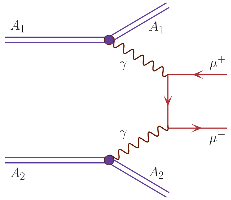
In Fig.1 we show the basic QED mechanism of the exclusive production of muon pairs. The shaded circles represent the coupling of photons to large-size objects – nuclei. In the momentum space this is done in terms of electromagnetic form factors of nuclei. In the case of scalar nuclei there is only one form factor – the charge form factor of the nucleus.

Refer to caption
Figure 1: (Color online) The Born diagram for the exclusive dimuon production.

It was recognized long ago that the production rate of leptons in ultrarelativistic heavy ion collisions is enhanced considerably by the coherent effects and large charge of colliding ions Budnev . Many results have been presented in the literature since then (for reviews of the field see e.g. BHTSK02 ; Baltz_review ). Recently, there was a growing theoretical interest in estimating higher-order QED corrections Nikolaev ; Serbo ; Baltz1 ; Baltz2 . In most of the practical calculations of exclusive dilepton production a simple monopole charge form factor of the nucleus was used. While it may be sufficient for estimating the total cross section, it may be not sufficient for calculations of the differential cross sections. The importance of including realistic charge form factors was discussed recently for exclusive production of pairs of $\rho^{0}$ mesons KSS09 .

Most of the existing calculations concentrated on total cross section, interesting theoretical quantity, which cannot be, however, measured in practice, neither at RHIC nor at LHC. The experiments running at RHIC and those planned at LHC demand severe cuts on lepton transverse momenta or on their rapidities.

It is the aim of the present analysis to make realistic estimates of the cross sections including the experimental cuts. We shall compare the results obtained with monopole form factor used in the literature and the results obtained with realistic form factor being Fourier transform of the charge density of the nucleus. We shall perform the calculation in the equivalent photon approximation (EPA) in the impact parameter space as well as in the momentum space. While the impact parameter EPA allows to include easily absorption effects due to the size of colliding nuclei, the momentum space approach allows to study easily several differential distributions. In our calculation we shall include experimental limitations of the STAR and PHENIX detectors at RHIC and those of the ALICE and CMS detectors at LHC.

II Formalism

II.1 Charge form factor of nuclei

The charge distribution in nuclei is usually obtained from elastic scattering of electrons from nuclei Barrett_Jackson . The charge distribution obtained from these experiments is often parametrized with the help of two–parameter Fermi model nuclear_density :

$$\rho\left(r\right)=\rho_{0}\left(1+exp\left(\frac{r-c}{a}\right)\right)^{-1},$$ (1)

where $c$ is the radius of the nucleus and $a$ is the so-called diffiusness parameter of the charge density.

Refer to caption
Figure 2: (Color online) The ratio of the charge distibution ($\rho$) to the density in the center of nucleus ($\rho_{0}$).

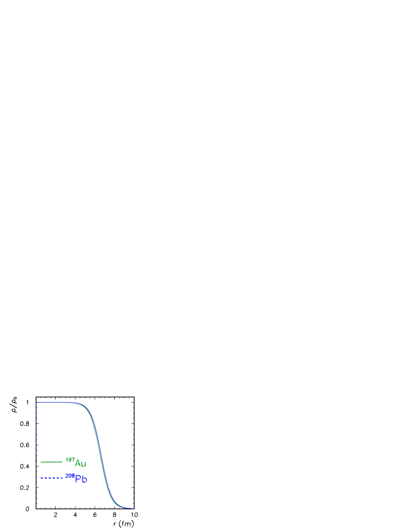
Fig. 2 shows the charge density normalizationed to unity at $r=0$. The correct normalization is: $\rho_{Au}(0)=\frac{0.1694}{A}fm^{-3}$ for Au nucleus and $\rho_{Pb}(0)=\frac{0.1604}{A}fm^{-3}$ for Pb nucleus.

Refer to caption
Figure 3: (Color online) The moduli of the charge form factor $F_{em}\left(q\right)$ of the ${}^{197}Au$ and ${}^{208}Pb$ nuclei for realistic charge distributions. For comparison we show the monopole form factor for the same nuclei.
Refer to caption
Figure 4: (Color online) The monopole form factor for the values of $\Lambda$ reproducing charge radius of ${}^{197}Au$ and ${}^{208}Pb$ nuclei and for comparison for $\Lambda=0.08$ GeV often used in the literature.

The form factor ($F$) is the Fourier transform of the charge distribution Barrett_Jackson . If $\rho\left(r\right)$ is spherically symmetric then the form factor is a function of photon virtuality ($q$) only:

$$F(q)=\int\frac{4\pi}{q}\rho\left(r\right)sin\left(qr\right)rdr=1-\frac{q^{2}\langle r^{2}\rangle}{3!}+\frac{q^{4}\langle r^{4}\rangle}{5!}\ldots\;.$$ (2)

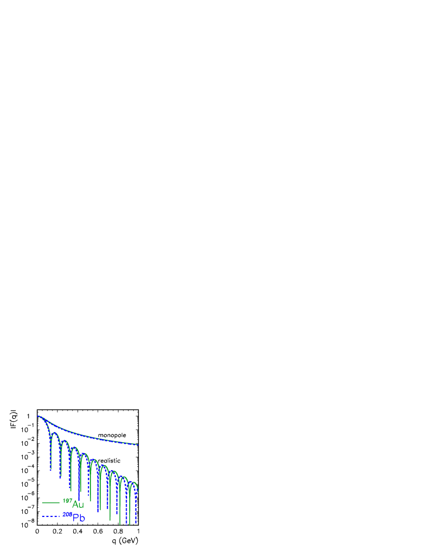
Fig. 4 shows the moduli of the form factor as a function of momentum transfer. The results are depicted for the gold (solid line) and lead (dashed line) nuclei for realistic charge distribution. The realistic form factor is obtained as a Fourier transform of the realistic charge density which we take from the literature Barrett_Jackson . Here one can see many oscillations characteristic for relatively sharp edge of the nucleus. For comparison we show the monopole form factor often used in the literature. The two form factors coincide only in a very limited range of $q$ and with larger value of $q$ the difference between them becomes larger and larger.

The monopole form factor HTB94 given by the simple formula:

$$F(q^{2})=\frac{\Lambda^{2}}{\Lambda^{2}+q^{2}}$$ (3)

leads to a simplification of many formulae for photon-photon collisions. In our calculation $\Lambda$ is adjusted to reproduce the root mean square radius of a nucleus ($\Lambda=\sqrt{\frac{6}{<r^{2}>}}$) with the help of experimental data nuclear_density :

  • for ${}^{197}Au$: $<r^{2}>^{1/2}=5.3\,\Rightarrow\,\Lambda=0.091\,\mbox{GeV}$,

  • for ${}^{208}Pb$: $<r^{2}>^{1/2}=5.5016\,\Rightarrow\,\Lambda=0.088\,\mbox{GeV}$.

Different values of $\Lambda$ are used in the literature, ranging from $80$ to $90$ MeV. Fig. 4 shows the monopole form factor with $\Lambda$ adjusted to reproduce the rms radius of the charge distribution.

II.2 Equivalent Photon Approximation

Refer to caption
Figure 5: (Color online) Equivalent photon approximation.
Refer to caption
Figure 6: (Color online) The quantities used in the impact parameter calculation.

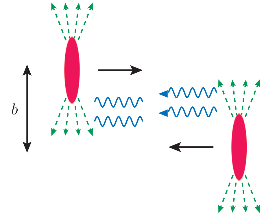
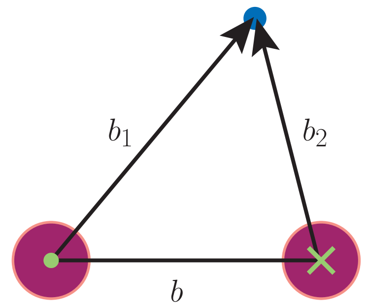
The equivalent photon approximation is the standard semi–classical alternative to the Feynman rules for calculating cross sections of electromagnetic interactions Jackson . This is illustrated in Fig. 6 where we can see a fast moving nucleus with the charge $Ze$. Due to the coherent action of all the protons in the nucleus, the electromagnetic field surrounding (the dashed lines are lines of electric force for a particles in motion) the ions is very strong. This field can be viewed as a cloud of virtual photons. These photons are often considered as real. They are called ”equivalent” or ”quasireal photons”. In the collision of two ions, these quasireal photons can collide with each other or with the other nucleus. So the strong electromagnetic field is used as a source of photons to induce electromagnetic reactions on the second ion. We consider very peripheral collisions. It means that the distance between nuclei is bigger than the sum of the radii of the two nuclei ($b>R_{1}+R_{2}\cong 14fm$). Fig. 6 explains the quantities used in the impact parameter calculation. We can see a view in the plane perpendicular to the direction of motion of the two ions. In order to calculate the cross section of a process it is convenient to introduce a new kinematic variable: $x=\frac{\omega}{E_{A}}$, where $\omega$ is the energy of the photon and the energy of the nucleus $E_{A}=\gamma Am_{proton}=\gamma M_{A}$, where $M_{A}$ is the mass of the nucleus and $\gamma$ is the Lorentz factor.

The total cross section can be calculated by the convolution:

$\displaystyle\sigma\left(AA\rightarrow\mu^{+}\mu^{-}AA;s_{AA}\right)=\int{\hat{\sigma}}\left(\gamma\gamma\rightarrow\mu^{+}\mu^{-};W_{\gamma\gamma}=\sqrt{x_{1}x_{2}s_{AA}}\right)\,{\rm d}n_{\gamma\gamma}\left(x_{1},x_{2},{\bf b}\right).$ (4)

The effective photon fluxes can be expressed through the electric fields generated by the nuclei:

$\displaystyle{\rm d}n_{\gamma\gamma}\left(x_{1},x_{2},{\bf b}\right)=$ $\displaystyle\frac{1}{\pi}{\rm d^{2}}{\bf b}_{1}|{\bf E}\left(x_{1},{\bf b}_{1}\right)|^{2}\frac{1}{\pi}{\rm d^{2}}{\bf b}_{2}|{\bf E}\left(x_{2},{\bf b}_{2}\right)|^{2}$ (5)
$\displaystyle\times$ $\displaystyle S^{2}_{abs}\left({\bf b}\right)\delta^{\left(2\right)}\left({\bf b}-{\bf b}_{1}+{\bf b}_{2}\right)\frac{{\rm d}x_{1}}{x_{1}}\frac{{\rm d}x_{2}}{x_{2}}.$

The presence of the absorption factor $S^{2}_{abs}\left({\bf b}\right)$ assures that we consider only peripheral collisions, when the nuclei do not undergo nuclear breakup. In the first approximation this can be expressed as:

$\displaystyle S^{2}_{abs}\left({\bf b}\right)=\theta\left({\bf b}-2R_{A}\right)=\theta\left(|{\bf b}_{1}-{\bf b}_{2}|-2R_{A}\right)\;.$ (6)

Thus in the present case, we concentrate on processes with final nuclei in the ground state. The electric field strength can be expressed through the charge form factor of the nucleus:

$\displaystyle{\bf E}\left(x,{\bf b}\right)=Z\sqrt{4\pi\alpha_{em}}\int\frac{{\rm d^{2}}{\bf q}}{\left(2\pi^{2}\right)}e^{-i{\bf bq}}\frac{{\bf q}}{{\bf q}^{2}+x^{2}M_{A}^{2}}F_{em}\left({\bf q}^{2}+x^{2}M_{A}^{2}\right).$ (7)

Next we can benefit from the following formal substitution:

$\displaystyle\frac{1}{\pi}\int{\rm d^{2}}{\bf b}|{\bf E}\left(x,{\bf b}\right)|^{2}=\int{\rm d^{2}}{\bf b}N\left(\omega,{\bf b}\right)\equiv n\left(\omega\right)\;$ (8)

by introducting effective photon fluxes which depend on energy of the quasireal photon $\omega$ and the distance from the nucleus in the plane perpendicular to the nucleus motion $\overrightarrow{b}$. Then, the luminosity function can be expressed in term of the photon flux factors attributed to each of the nuclei

$\displaystyle{\rm d}n_{\gamma\gamma}\left(\omega_{1},\omega_{2},{\bf b}\right)$ $\displaystyle=$ $\displaystyle\int\theta\left(|{\bf b}_{1}-{\bf b}_{2}|-2R_{A}\right)N\left(\omega_{1},{\bf b}_{1}\right)N\left(\omega_{2},{\bf b}_{2}\right){\rm d^{2}}{\bf b}_{1}{\rm d^{2}}{\bf b}_{2}{\rm d}\omega_{1}{\rm d}\omega_{2}.$ (9)

The total cross section for the $AA\rightarrow\mu^{+}\mu^{-}AA$ process can be factorized into the equivalent photons spectra ( $n\left(\omega\right)$ ) and the $\gamma\gamma\to\mu^{+}\mu^{-}$ subprocess cross section as (see e.g.BF91 ):

$\displaystyle\sigma\left(AA\rightarrow\mu^{+}\mu^{-}AA;s_{AA}\right)$ $\displaystyle=$ $\displaystyle\int{\hat{\sigma}}\left(\gamma\gamma\rightarrow\mu^{+}\mu^{-};W_{\gamma\gamma}\right)\,\theta\left(|{\bf b}_{1}-{\bf b}_{2}|-2R_{A}\right)$ (10)
$\displaystyle\times$ $\displaystyle N\left(\omega_{1},{\bf b}_{1}\right)N\left(\omega_{2},{\bf b}_{2}\right){\rm d^{2}}{\bf b}_{1}{\rm d^{2}}{\bf b}_{2}{\rm d}\omega_{1}{\rm d}\omega_{2}\;,$

where $W_{\gamma\gamma}=\sqrt{4\omega_{1}\omega_{2}}$ is energy in the $\gamma\gamma$ subsystem. Eq. (10) is a generalization of the simple parton model formula (see e.g.BHTSK02 ):

$$\sigma\left(AA\rightarrow\mu^{+}\mu^{-}AA\right)=\int{\hat{\sigma}}\left(\gamma\gamma\rightarrow\mu^{+}\mu^{-};\sqrt{4\omega_{1}\omega_{2}}\right)n\left(\omega_{1}\right)n\left(\omega_{2}\right){\rm d}\omega_{1}{\rm d}\omega_{2}\;.$$ (11)

Additionally, we define $Y=\frac{1}{2}\left(y_{\mu^{+}}+y_{\mu^{-}}\right)$, rapidity of the outgoing dimuon system which is produced in the photon–photon collision. Performing the following transformations:

$$\omega_{1}=\frac{W_{\gamma\gamma}}{2}e^{Y},\qquad\omega_{2}=\frac{W_{\gamma\gamma}}{2}e^{-Y}\;,$$ (12)
$${\rm d}\omega_{1}{\rm d}\omega_{2}=\frac{W_{\gamma\gamma}}{2}{\rm d}W_{\gamma\gamma}{\rm d}Y\;,$$ (13)
$${\rm d}\omega_{1}{\rm d}\omega_{2}\to{\rm d}W_{\gamma\gamma}{\rm d}Y\mbox{ where }\left|\frac{\partial\left(\omega_{1},\omega_{2}\right)}{\partial\left(W_{\gamma\gamma},Y\right)}\right|=\frac{W_{\gamma\gamma}}{2}\;,$$ (14)

formula (10) can be rewritten as:

$\displaystyle\sigma\left(AA\rightarrow\mu^{+}\mu^{-}AA;s_{AA}\right)=\int{\hat{\sigma}}\left(\gamma\gamma\rightarrow\mu^{+}\mu^{-};W_{\gamma\gamma}\right)\theta\left(|{\bf b}_{1}-{\bf b}_{2}|-2R_{A}\right)$
$\displaystyle\times N\left(\omega_{1},{\bf b}_{1}\right)N\left(\omega_{2},{\bf b}_{2}\right)\frac{W_{\gamma\gamma}}{2}{\rm d^{2}}{\bf b}_{1}{\rm d^{2}}{\bf b}_{2}{\rm d}W_{\gamma\gamma}{\rm d}Y$ . (15)

Finally, the cross section can be expressed as the five-fold integral:

$\displaystyle\sigma\left(AA\rightarrow\mu^{+}\mu^{-}AA;s_{AA}\right)=\int{\hat{\sigma}}\left(\gamma\gamma\rightarrow\mu^{+}\mu^{-};W_{\gamma\gamma}\right)\theta\left(|{\bf b}_{1}-{\bf b}_{2}|-2R_{A}\right)$
$\displaystyle\times N\left(\omega_{1},{\bf b}_{1}\right)N\left(\omega_{2},{\bf b}_{2}\right)2\pi b_{m}\,{\rm d}b_{m}\,{\rm d}\overline{b}_{x}\,{\rm d}\overline{b}_{y}\frac{W_{\gamma\gamma}}{2}{\rm d}W_{\gamma\gamma}{\rm d}Y$ , (16)

where $\overline{b}_{x}\equiv(b_{1x}+b_{2x})/2$, $\overline{b}_{y}\equiv(b_{1y}+b_{2y})/2$ and $\vec{b}_{m}=\vec{b}_{1}-\vec{b}_{2}$ have been introduced. This formula is used to calculate the total cross section for the $AA\to AA\mu^{+}\mu^{-}$ reaction as well as the distributions in $b=b_{m}$, $W_{\gamma\gamma}=M_{\mu^{+}\mu^{-}}$ and $Y(\mu^{+}\mu^{-})$.

Different forms of form factors are used in the literature. We compare the equivalent photon spectra for an extended charge distribution (realistic case) to the monopole case. The dependence of the photon flux on the charge form factors can be found in BHTSK02 :

$$N\left(\omega,b\right)=\frac{Z^{2}\alpha_{em}}{\pi^{2}}\frac{1}{b^{2}\omega}\left(\int u^{2}J_{1}\left(u\right)F\left(\sqrt{\frac{\left(\frac{b\omega}{\gamma}\right)^{2}+u^{2}}{b^{2}}}\right)\frac{1}{\left(\frac{b\omega}{\gamma}\right)^{2}+u^{2}}du\right)^{2},$$ (17)

where $J_{1}$ is the Bessel function of the first kind and $q$ is the four-momentum of the quasireal photon. The calculations with the help of realistic form factor are rather laborious, so often a simpler monopole form factor is used HTB94 . Introducing monopole form factor to (17) one gets:

$$N\left(\omega,b\right)=\frac{Z^{2}\alpha_{em}}{\pi^{2}}\frac{1}{\omega}\left(\frac{\omega}{\gamma}K_{1}\left(\frac{b\omega}{\gamma}\right)-\sqrt{\frac{\omega^{2}}{\gamma^{2}}+\Lambda^{2}}\;K_{1}\left(b\sqrt{\frac{\omega^{2}}{\gamma^{2}}+\Lambda^{2}}\right)\right)^{2}\;,$$ (18)

where $K_{1}$ is the modified Bessel function of the second kind.

Refer to caption
Figure 7: (Color online) The equivalent photon number as a function of impact parameter (integrated over $\omega$), see Eq. (19).
Refer to caption
Figure 8: (Color online) The ratio of the flux factor obtained with realistic charge distribution to that with the monopole form factor as a function of impact parameter.
Refer to caption
Refer to caption
Figure 9: (Color online) The equivalent photon number $n\left(\omega\right)$, see Eq. (20). Left panel: $b\in(0,100)$ fm, right panel: $b\in(14,100)$ fm.

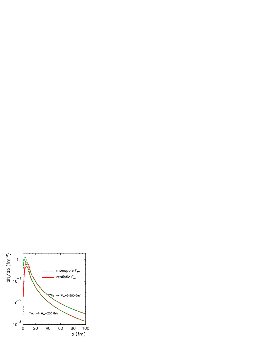
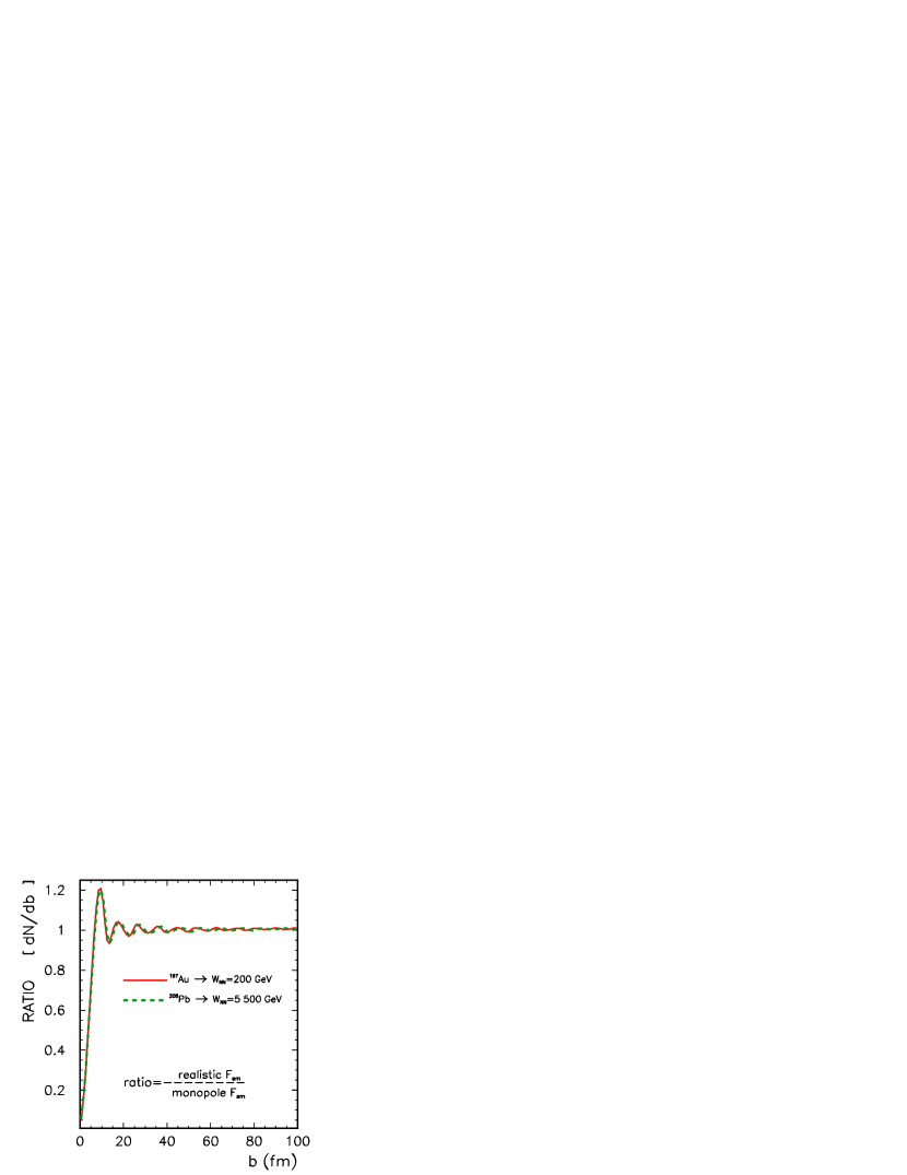
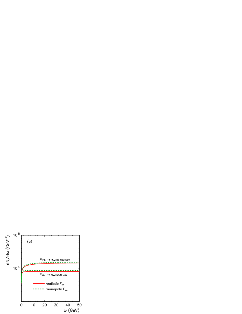
Fig. 7 shows the distribution of the equivalent photon number as a function of the impact parameter

$$N\left(b\right)=\int N\left(\omega,\,b\right)d\omega.$$ (19)

We present the results for gold and lead nuclei, for realistic and monopole form factors. Here we do not impose any sharp cutoff on the impact parameter. One can see that for small $b$ the flux factor with monopole form factor is bigger. For large $b$ the results obtained with the help of realistic and monopole form factors are almost the same.

In addition in Fig. 8 we show the ratio of equivalent photon fluxes obtained with the help of realistic form factor to that for the monopole form factor. The oscillations in $b$ are due to step-like distribution of the charge in the nucleus. The results for lower ($\sqrt{s}_{NN}=200$ GeV) and higher ($\sqrt{s}_{NN}=5.5$ TeV) energies are almost the same.

Fig. 9 shows

$$N\left(\omega\right)=\int 2\pi bN\left(\omega,\,b\right)db.$$ (20)

Here we consider the integral over full range of the impact parameter (left panel) and for $b>2R_{A}$ (right panel). One can see that the difference between monopole and realistic form factor for both gold and lead nuclei is not significant. The quantity shown depends rather weakly on the photon energy.

Refer to caption
Figure 10: (Color online) The elementary cross section for the $\gamma\gamma\to\mu^{+}\mu^{-}$ reaction as a function of the photon-photon energy.

In Fig. 10 we show the energy dependence of the elementary $\gamma\gamma\to\mu^{+}\mu^{-}$ cross section used in our EPA calculations Budnev :

$\displaystyle\sigma\left(\gamma\gamma\to\mu^{+}\mu^{-}\right)$ $\displaystyle=$ $\displaystyle\frac{4\pi\alpha_{em}^{2}}{W_{\gamma\gamma}^{2}}$
$\displaystyle\times$ $\displaystyle\left\{2\ln\left[\frac{W_{\gamma\gamma}}{2m_{\mu}}\left(1+v\right)\right]\left(1+\frac{4m_{\mu}^{2}W_{\gamma\gamma}^{2}-8m_{\mu}^{4}}{W_{\gamma\gamma}^{4}}\right)-\left(1+\frac{4m_{\mu}^{2}W_{\gamma\gamma}^{2}}{W_{\gamma\gamma}^{4}}\right)v\right\}\,,$

where

$$v=\sqrt{1-\frac{4m_{\mu}^{2}}{W_{\gamma\gamma}^{2}}}\;.$$ (22)

This formula is often called the Breit-Wheeler formula.

II.3 Momentum space calculation
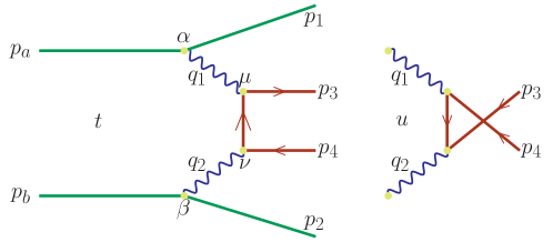
Refer to caption
Figure 11: (Color online) Amplitude of the considered process. On the left one can see the $t$-channel amplitude and on the right - the $u$-channel amplitude.

We consider a genuine $2\to 4$ reaction (see Fig. 11) with four-momenta $p_{a}+p_{b}\to p_{1}+p_{2}+p_{3}+p_{4}$. In the momentum space approach the cross section for the production of a pair of particles can be written as:

$\displaystyle\sigma$ $\displaystyle=$ $\displaystyle\int\frac{1}{2s}\overline{|\mathcal{M}|^{2}}\left(2\pi\right)^{4}\delta^{4}\left(p_{a}+p_{b}-p_{1}-p_{2}-p_{3}-p_{4}\right)$ (23)
$\displaystyle\times$ $\displaystyle\frac{d^{3}p_{1}}{\left(2\pi\right)^{3}2E_{1}}\frac{d^{3}p_{2}}{\left(2\pi\right)^{3}2E_{2}}\frac{d^{3}p_{3}}{\left(2\pi\right)^{3}2E_{3}}\frac{d^{3}p_{4}}{\left(2\pi\right)^{3}2E_{4}}\;.$

Using

$$\frac{d^{3}p_{i}}{E_{i}}=dy_{i}\,d^{2}p_{it}=dy_{i}p_{it}dp_{it}d\phi_{i}\;$$ (24)

Eq. (23) can be rewritten as:

$\displaystyle\sigma$ $\displaystyle=$ $\displaystyle\int\frac{1}{2s}\overline{|\mathcal{M}|^{2}}\delta^{4}\left(p_{a}+p_{b}-p_{1}-p_{2}-p_{3}-p_{4}\right)\frac{1}{\left(2\pi\right)^{8}}\frac{1}{2^{4}}$ (25)
$\displaystyle\times$ $\displaystyle\left(dy_{1}p_{1t}dp_{1t}d\phi_{1}\right)\left(dy_{2}p_{2t}dp_{2t}d\phi_{2}\right)\left(dy_{3}d^{2}p_{3t}\right)\left(dy_{4}d^{2}p_{4t}\right)\;.$

In the above formula $p_{it}$ are transverse momenta of outgoing nuclei and leptons, $\phi_{1}$, $\phi_{2}$ are azimuthal angles of outgoing nuclei. Additionally, we introduce a new auxiliary quantity

$${\bf p}_{m}={\bf p}_{3t}-{\bf p}_{4t}$$ (26)

and benefitting from 4-dimensional Dirac delta function properties, Eq. (25) can be written as:

$\displaystyle\sigma$ $\displaystyle=$ $\displaystyle\int\frac{1}{2s}\overline{|\mathcal{M}|^{2}}\delta\left(E_{a}+E_{b}-E_{1}-E_{2}-E_{3}-E_{4}\right)\delta^{3}\left(p_{1z}+p_{2z}+p_{3z}+p_{4z}\right)\frac{1}{\left(2\pi\right)^{8}}\frac{1}{2^{4}}$ (27)
$\displaystyle\times$ $\displaystyle\left(dy_{1}p_{1t}dp_{1t}d\phi_{1}\right)\left(dy_{2}p_{2t}dp_{2t}d\phi_{2}\right)dy_{3}dy_{4}d^{2}p_{m}\;.$

The energy-momentum conservation gives the following system of equations that has to be solved for discrete solutions

$\displaystyle\left\{\begin{array}[]{rll}&\sqrt{s}-E_{3}-E_{4}&=\sqrt{m_{1t}^{2}+p_{1z}^{2}}+\sqrt{m_{2t}^{2}+p_{2z}^{2}}\;,\\ &-p_{3z}-p_{4z}&=p_{1z}+p_{2z}\;,\\ \end{array}\right.$ (30)

where $m_{1t}$, $m_{2t}$ are the so-called transverse masses of outgoing nuclei which are defined as:

$$m_{it}^{2}=p_{it}^{2}+m_{i}^{2}\;.$$ (31)

We wish to make the transformation from $\left(y_{1},\,y_{2}\right)$ to $\left(p_{1z},\,p_{2z}\right)$. The transformation Jacobian takes the form:

$$\mathcal{J}_{k}=\left|\frac{p_{1z}\left(k\right)}{\sqrt{m_{1t}^{2}+p_{1z}^{2}\left(k\right)}}-\frac{p_{2z}\left(k\right)}{\sqrt{m_{2t}^{2}+p_{2z}^{2}\left(k\right)}}\right|\;,$$ (32)

where $k$ numerates discrete solutions of Eq. (30). Thus the cross section for the $2\to 4$ reaction reads:

$\displaystyle\sigma$ $\displaystyle=$ $\displaystyle\int\sum_{k}\mathcal{J}_{k}^{-1}\left(p_{1t},\,\phi_{1},\,p_{2t},\,\phi_{2},\,y_{3},\,y_{4},\,p_{m},\,\phi_{m}\right)\frac{1}{2\sqrt{s\left(s-4m^{2}\right)}}\overline{|\mathcal{M}|^{2}}\frac{1}{\left(2\pi\right)^{8}}\frac{1}{2^{4}}$ (33)
$\displaystyle\times$ $\displaystyle\left(p_{1t}dp_{1t}d\phi_{1}\right)\left(p_{2t}dp_{2t}d\phi_{2}\right)\frac{1}{4}dy_{3}dy_{4}d^{2}p_{m}\;.$

For photon-exchanges, considered here, it is convenient to change the variables $p_{1t}\to\xi_{1}=\log_{10}\left(p_{1t}\right)$, $p_{2t}\to\xi_{2}=\log_{10}\left(p_{2t}\right)$. The lepton helicity dependent amplitudes of the process shown in Fig. 11 can be written as:

$\displaystyle{\cal M}_{\lambda_{3},\lambda_{4}}\left(t\mbox{-channel}\right)$ $\displaystyle=$ $\displaystyle e\,F_{ch}\left(q_{1}\right)\,\left(p_{a}+p_{1}\right)^{\alpha}\frac{-i\,g_{\alpha\mu}}{q_{1}^{2}+i\varepsilon}\bar{u}\left(p_{3},\,\lambda_{3}\right)\,i\,\gamma^{\mu}\frac{i\,\left[\left(\not{p}_{3}-\not{q}_{1}\right)+m_{\mu}\right]}{\left(q_{1}-p_{3}\right)^{2}-m_{\mu}^{2}}$ (34)
$\displaystyle\times$ $\displaystyle i\,\gamma^{\nu}\,v\left(p_{4},\,\lambda_{4}\right)\,\frac{-i\,g_{\nu\beta}}{q_{2}^{2}+i\varepsilon}\,\left(p_{b}+p_{2}\right)^{\beta}\,e\,F_{ch}\left(q_{2}\right)$

and

$\displaystyle{\cal M}_{\lambda_{3},\lambda_{4}}\left(u\mbox{-channel}\right)$ $\displaystyle=$ $\displaystyle e\,F_{ch}\left(q_{1}\right)\,\left(p_{a}+p_{1}\right)^{\alpha}\frac{-i\,g_{\alpha\mu}}{q_{1}^{2}+i\varepsilon}\bar{u}\left(p_{3},\,\lambda_{3}\right)\,i\,\gamma^{\nu}\frac{i\,\left[\left(\not{p}_{3}-\not{q}_{2}\right)+m_{\mu}\right]}{\left(q_{2}-p_{3}\right)^{2}-m_{\mu}^{2}}$ (35)
$\displaystyle\times$ $\displaystyle i\,\gamma^{\mu}\,v\left(p_{4},\,\lambda_{4}\right)\,\frac{-i\,g_{\nu\beta}}{q_{2}^{2}+i\varepsilon}\,\left(p_{b}+p_{2}\right)^{\beta}\,e\,F_{ch}\left(q_{2}\right)\;.$

These amplitudes are calculated numerically. Finally, to calulate the total cross section one has to calculate the 8-dimensional integral inserting ${\cal M}_{\lambda_{3},\lambda_{4}}={\cal M}_{\lambda_{3},\lambda_{4}}\left(t\mbox{-channel}\right)+{\cal M}_{\lambda_{3},\lambda_{4}}\left(u\mbox{-channel}\right)$ into Eq. (33). We shall compare the impact parameter EPA results with the exact 111By exact we mean the correct inclusion of the $2\to 4$ process phase-space. It is, however, rather difficult to include absorption effects in this approach. Quantum Electrodynamics results.

III Results

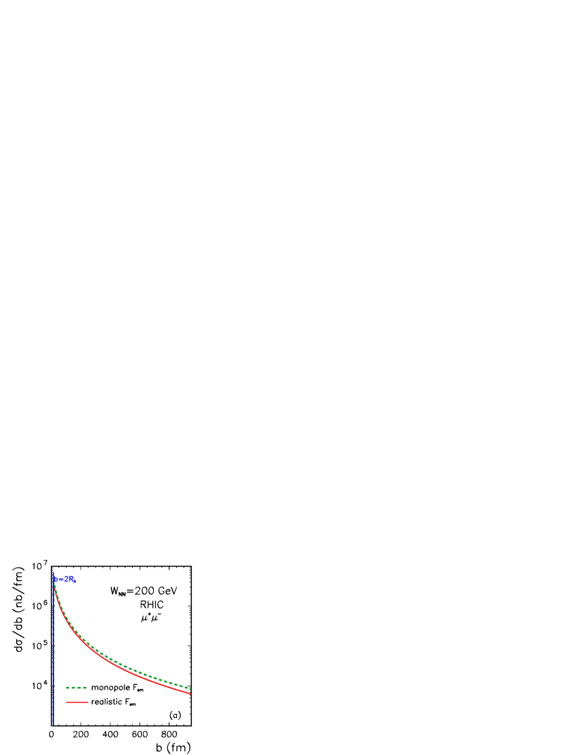
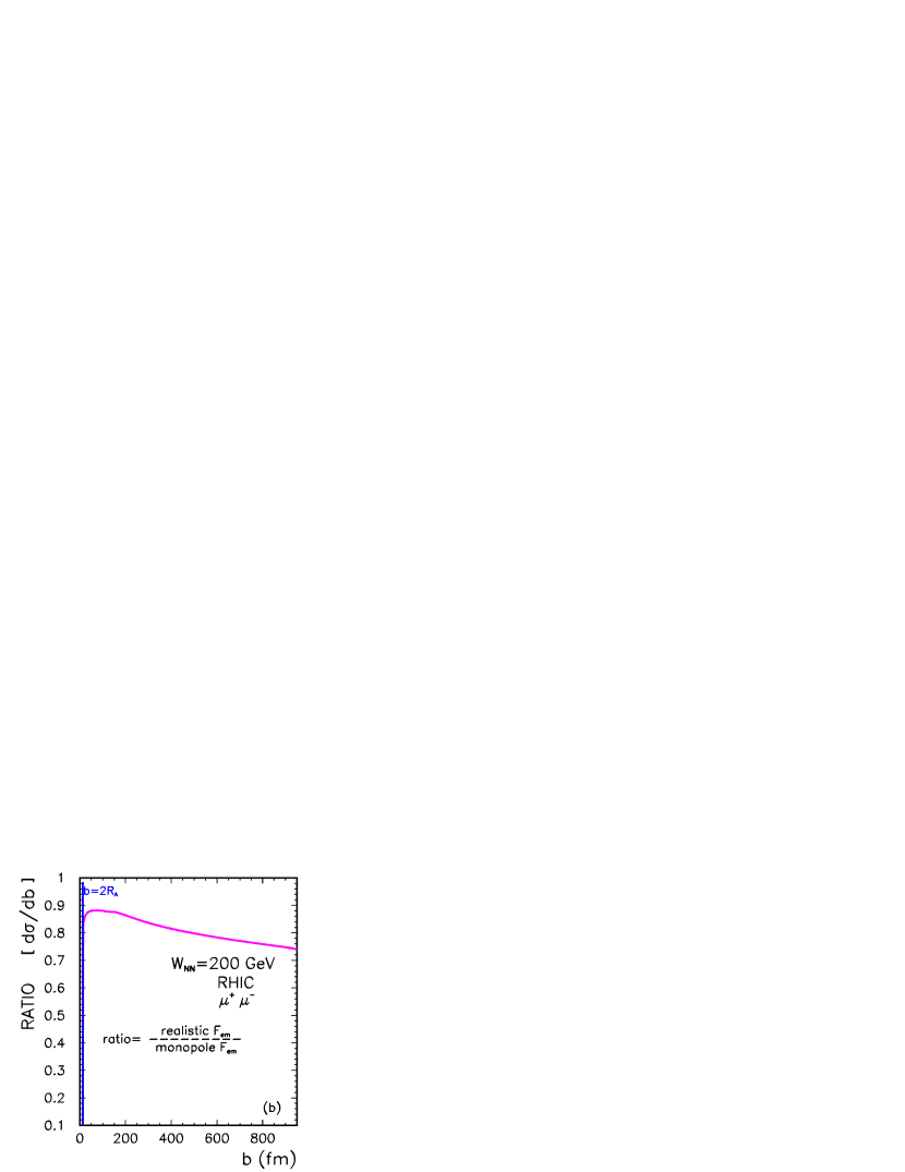
Let us start from the presentation of the results obtained in the impact parameter EPA. In Fig.12 we show the distribution in the impact parameter $b$ for typical RHIC energy $\sqrt{s_{NN}}$ = 200 GeV. The contributions from distances smaller than $b=2R_{A}$ are cut off and consistently with $\theta$-function in Eq. (16). We clearly see a huge contribution from distances large compared to the nuclear size. The distribution with realistic charge falls off somewhat quicker than that for the monopole charge form factor. This is better visualized in the right panel where the ratio of the corresponding cross sections is shown.

Refer to caption
Refer to caption
Figure 12: (Color online) The cross section as a function of the impact parameter for the $AuAu\to\mu^{+}\mu^{-}AuAu$ reaction calculated in the equivalent photon approximation. In the left panel we show the results for realistic charge distribution (solid line) and for monopole form factor (dashed line). On the right side we depict the ratio : $RATIO={\rm d}\sigma\left(F_{em}^{REALISTIC}\right)/{\rm d}\sigma\left(F_{em}^{MONOPOLE}\right)$.
Refer to caption
Refer to caption
Figure 13: $\frac{{\rm d}\sigma}{{\rm d}b_{1}{\rm d}b_{2}}$ as a function of $b_{1}$ and $b_{2}$ in lego (left) and contour (right) representation for $b\in$ (480,520) fm.

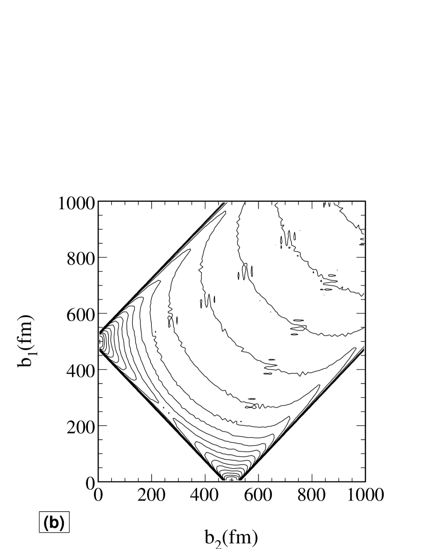
The difference of the cross sections for the monopole and exact charge form factors at large impact parameter $b$ shown in the figure is especially intriguing in the light of the equality of the photon flux factors at large $b_{1}$ or $b_{2}$ (see Fig.7). How to understand this quite nonintuitive result? In Fig.13 we show the distribution of $d\sigma/db_{1}db_{2}$ in ($b_{1},b_{2}$) with the severe restriction for the impact parameter $b\in$ (480,520) fm. We see two pronounced peaks at ($b_{1}\approx b,b_{2}\approx 0$) and ($b_{1}\approx 0,b_{2}\approx b$). This demonstrates a strong preference of asymmetric production of the pair: close to the trajectory of one or the other nucleus, where the form factor details are important (see Fig.7). This point was never discussed so far in the literature.

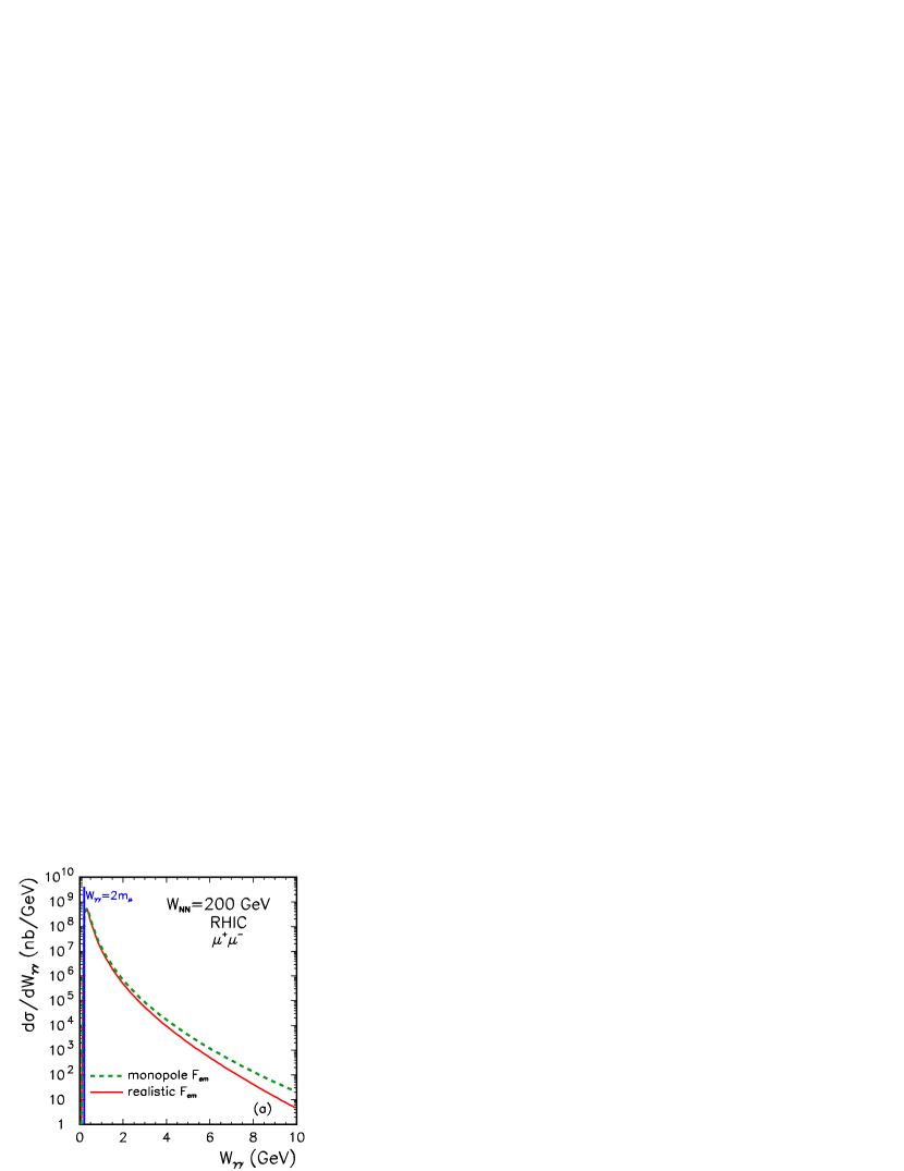
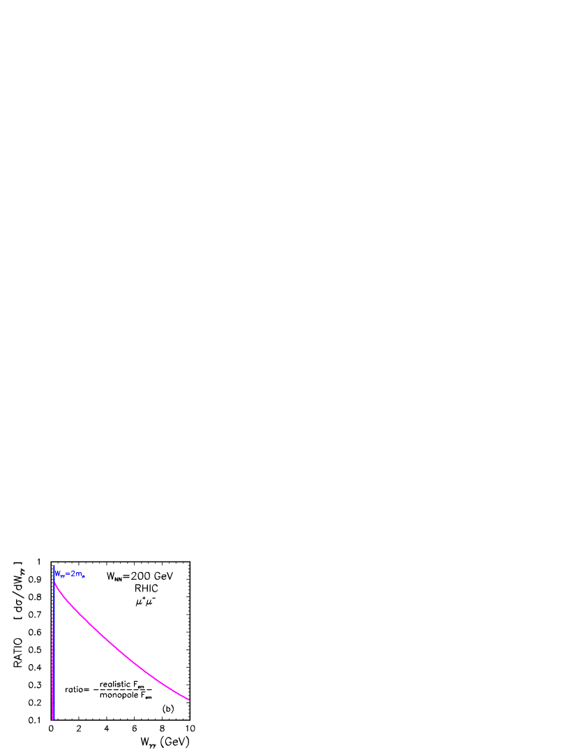
The distributions shown in Fig.12 are purely theoretical, that is cannot be easily measured. Let us come now to the distributions which could, at least in principle, be measured. Fig.14 shows the distribution in the dimuon subsystem energy. The distributions in $W_{\gamma\gamma}=M_{\mu^{+}\mu^{-}}$ falls steeply off. In the right panel we show the ratio of the cross sections for realistic charge distribution to that for the monopole charge form factor. At $W_{\gamma\gamma}$ = 10 GeV the two distributions differ already by a factor of about 5 which clearly shows limitations of the calculations with analytic charge form factors.
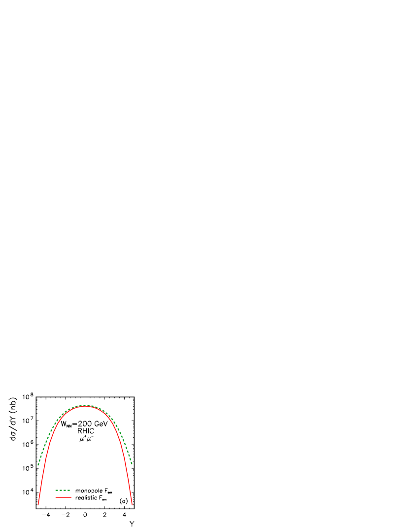
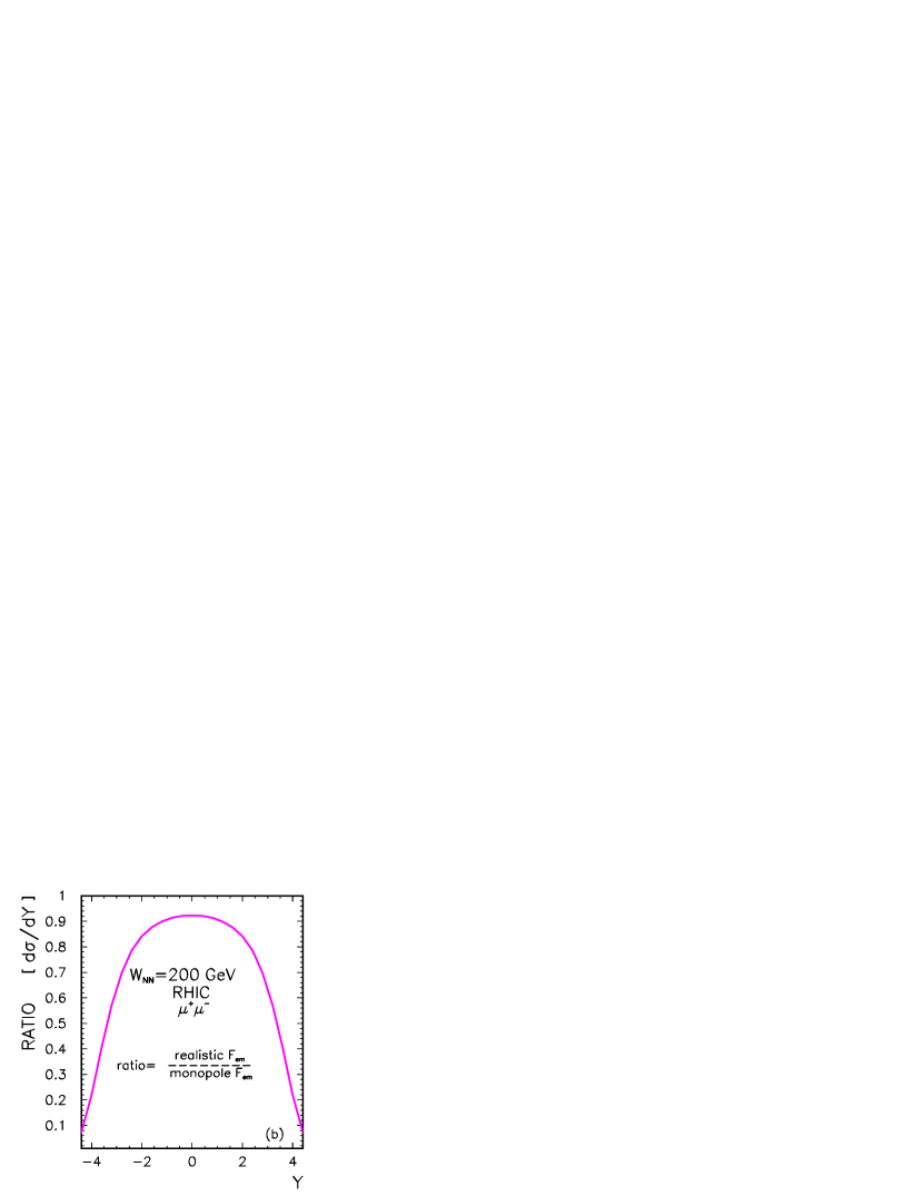
Refer to caption
Refer to caption
Figure 14: (Color online) The cross section for $Au-Au$ scattering as a function of photon–photon center–of–mass energy $W_{\gamma\gamma}=M_{\mu^{+}\mu^{-}}$ in EPA. In the right panel we show the ratio of ”realistic” to ”monopole” form factor.

Finally, in analogy to the $AA\to AA\rho^{0}\rho^{0}$ reaction studied in Ref.KSS09 , in Fig.15 we show the distribution in the dimuon pair rapidity. As for the $\rho^{0}\rho^{0}$ production we see a huge difference between the results of the two calculations for large dilepton rapidities. Measurements of dileptons in forward directions would be therefore very useful to understand the role of realistic charge distribution. The relative effect is shown in the right panel of the figure.

Refer to caption
Refer to caption
Figure 15: (Color online) The cross section as a function of $Y=\frac{1}{2}\left(y_{\mu^{+}}+y_{\mu^{-}}\right)$ (left panel) for realistic and monopole form factors (left) calculated in EPA and their ratio (right).

The preliminary calculation in the impact parameter space clearly shows how important can be studying of differential distributions to pin down the effects of realistic charge density. Not all of the distributions can be easily addressed in the impact parameter approach. The Feynman diagram approach in the momentum space seems to be a better alternative to study the differential distributions.

Now we come to the presentation of results obtained in the momentum space approach with details outlined in Section II. Fig.16 shows distributions in muon rapidities (identical for $\mu^{+}$ and $\mu^{-}$). No other limitations or kinematical cuts have been included here. As in the previous cases we show distributions obtained with the monopole and realistic charge form factor. The effect of the oscillatory character of $F_{ch}(q)$ and in particular its first minimum is reflected by a smaller cross section at larger rapidities compared to the results obtained with monopole form factor. This is due to the fact that on average at large rapidities larger four-momentum squared transfers ($t_{1}$ or $t_{2}$) are involved. In reality, one effectively integrates over a certain range of $t_{1}$ and $t_{2}$. The relative effect is shown in the right panel.

Refer to caption
Refer to caption
Figure 16: (Color online) The cross section as a function of $y_{\mu^{+}}$, $y_{\mu^{-}}$ for realistic and monopole form factor calculated in the momentum space (left panel). Their ratio is shown in the right panel.

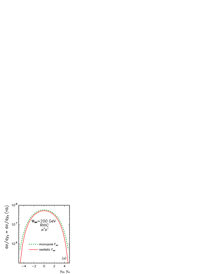
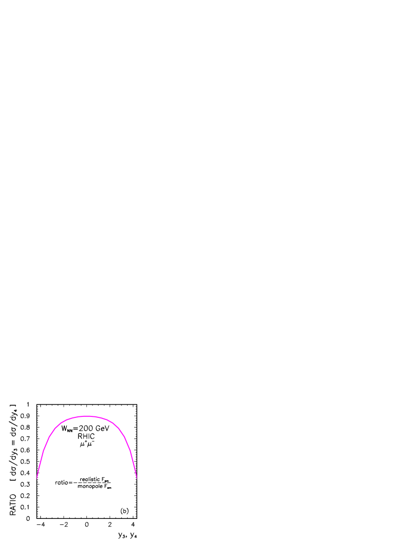
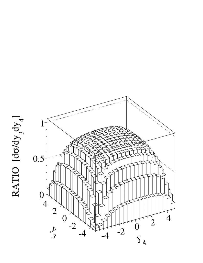
Fig.17 shows the situation (the ratio of the two calculations) in the two dimensional space: ($y_{3},y_{4}$). Clearly at mid rapidities, where on average rather small $t_{1}$ and $t_{2}$ are involved, the use of the approximate monopole form factor is justified. This is not the case at the edges of the ($y_{3},y_{4}$) plane where due to kinematics $\left|t_{1}\right|$ or/and $\left|t_{2}\right|$ are larger.

Refer to caption
Figure 17: The ratio of two-dimensial distributions ${\rm d}\sigma\left(F_{em}^{REALISTIC}\right)/{\rm d}\sigma\left(F_{em}^{MONOPOLE}\right)$ in $y_{3}$ and $y_{4}$.

Up to now we have discussed ”a theoretical situation” when all the muons are accepted. In practice one can measure only muons with transverse momenta larger than a certain value, characteristic for a given detector. We shall consider now cases relevant for concrete experimental situations.

Refer to caption
Figure 18: (Color online) The compilation of the results obtained in different approaches for the total cross section for $AuAu\to AuAu\mu^{+}\mu^{-}$ at $\sqrt{s}_{NN}$ = 200 GeV.

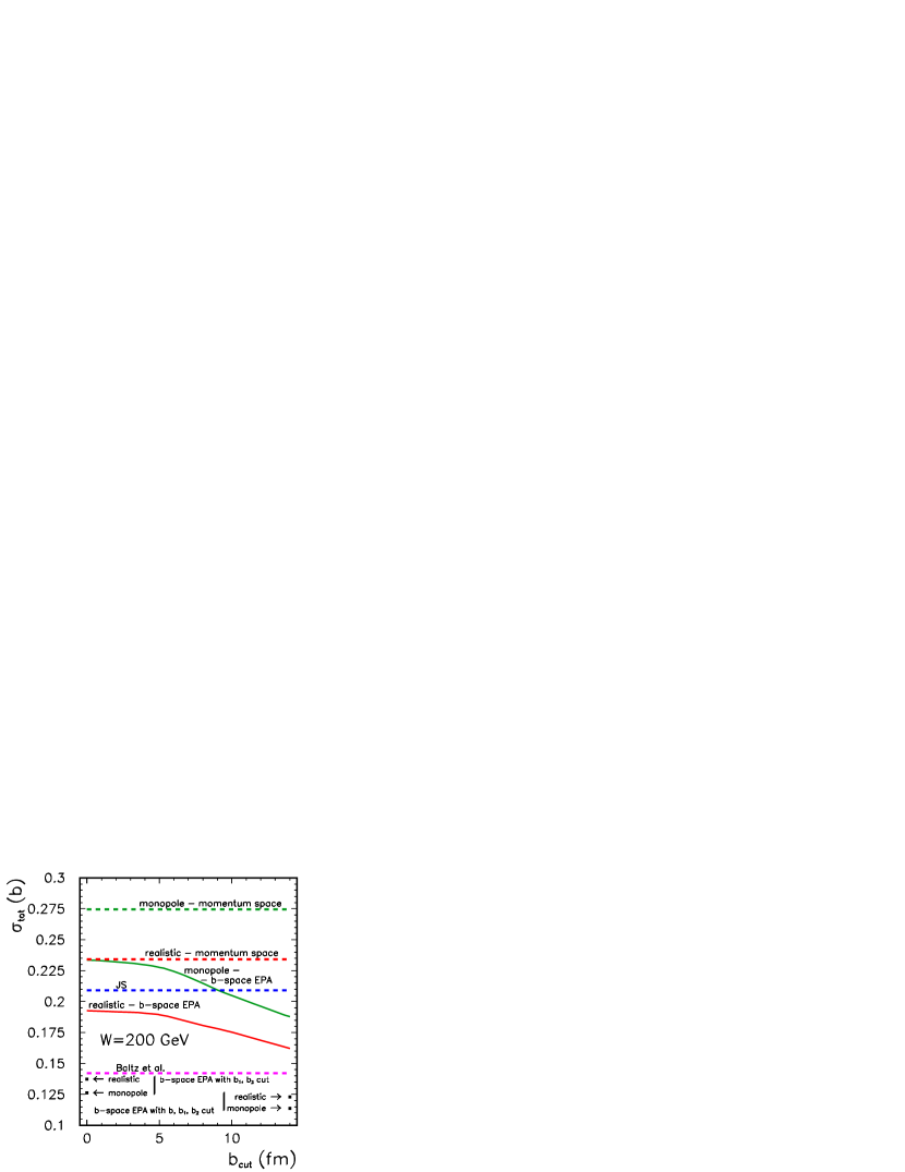
The calculations in the literature concentrated mostly on the total cross section. In Fig.18 we present the dependence of the total cross section on the lower cut-off in the impact parameter. We present EPA results for realistic (lower solid line) and monopole (upper solid line) form factors. The cross section without the cut-off is by 15% larger than that for $b_{cut}$ = 14 fm. This result is smaller than the corresponding results obtained within momentum space calculations, shown as the horizontal dashed lines. Different methods has been used in the literature to calculate the total cross section for the $AuAu\to AuAu\mu^{+}\mu^{-}$ process. For comparison we show also results obtained recently by Jentschura and Serbo (JS) SB in the momentum space EPA and by Baltz et al. BGKN09 in the b-space EPA. The JS result should be compared to our momentum space calculation with monopole form factor. Our exact calculation is in this case larger than their EPA calculation by about 24%. This shows the precision of the momentum space EPA. The Baltz et al. result is significantly lower than our b-space EPA result. In their calculations the cuts were imposed rather on $b_{1}$ and $b_{2}$, instead on $b$ in our case. If we impose additional cuts on $b_{1}$ and $b_{2}$ in Eq. (16) we get the point in the lower-right corner. If the cut on $b$ is not imposed we get the point in the lower-left corner. The result of Baltz et al. differs from both these values, the solution being most probably a different form factor used in their case.

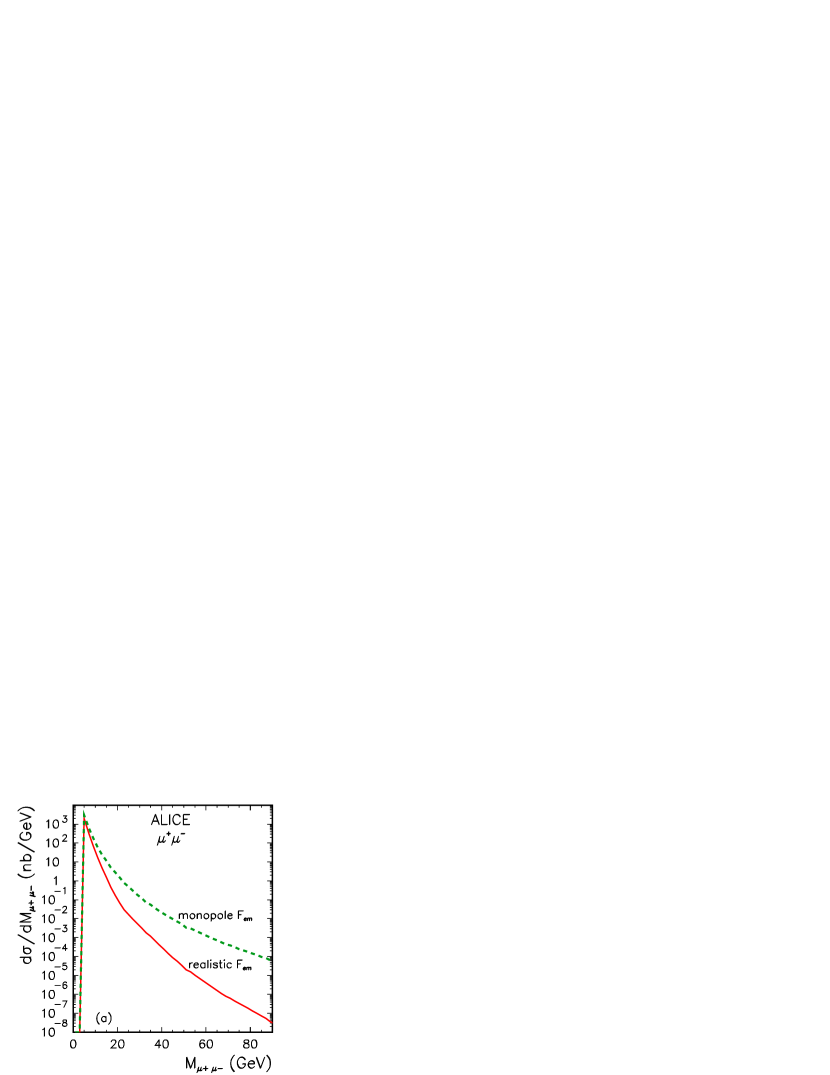
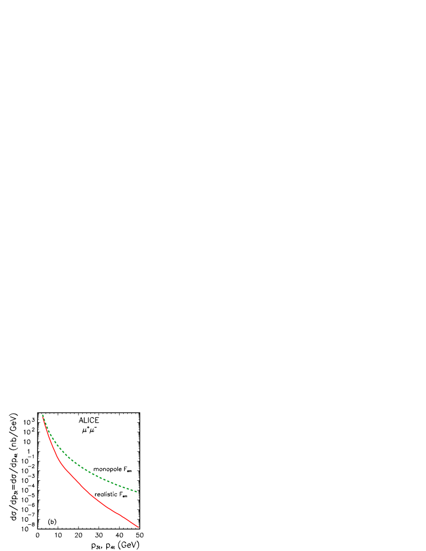
Now we will continue reviewing our predictions for the differential distributions. Let us start with the ALICE detector. The ALICE collaboration can measure only forward muons with psudorapidity 4 $<\eta<$ 5 and uses a relatively low cut on muon transverse momentum, $p_{t}>$ 2 GeV. In Fig.19 (left panel) we show the invariant mass distribution of dimuons for monopole and realistic form factors. The ALICE experimental cuts were incorporated into our calculations. The bigger invariant mass the bigger the difference between the results for the two form factors. The same is true for distributions in muon transverse momenta (see the right panel).

Refer to caption
Refer to caption
Figure 19: (Color online) Invariant mass distribution $\frac{{\rm d}\sigma}{{\rm d}M_{\mu^{+}\mu^{-}}}$ (left) and muon transverse momentum distribution $\frac{{\rm d}\sigma}{{\rm d}p_{3t}}=\frac{{\rm d}\sigma}{{\rm d}p_{4t}}$ (right) for ALICE conditions: $y_{3},y_{4}\in(3,4)$, $p_{3t},p_{4t}\geq$ 2 GeV and the center-of-mass energy $W_{NN}=5.5$ TeV.

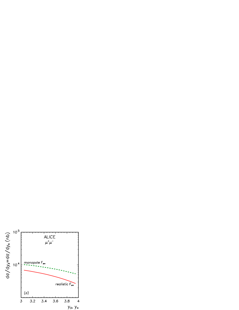
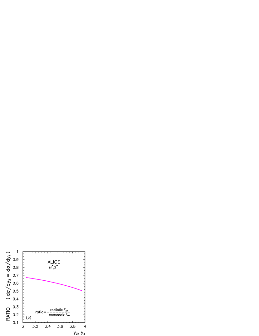
The distribution in rapidity is shown in Fig.20. We present the cross sections for both (realistic, monopole) form factors and their ratio.

Refer to caption
Refer to caption
Figure 20: (Color online) $\frac{{\rm d}\sigma}{{\rm d}y_{3}}=\frac{{\rm d}\sigma}{{\rm d}y_{4}}$ (left) and their ratio (right) for the ALICE conditions: $y_{3},y_{4}\in(3,4)$, $p_{3t},p_{4t}\geq$ 2 GeV and $W_{NN}=5.5$ TeV.

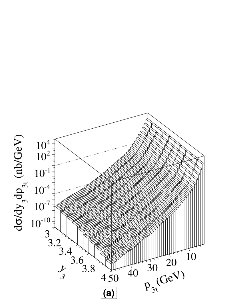
Double differential distribution of the muon rapidity and transverse momentum is shown in Fig.21. These are our predictions which could be studied experimentally in the future. The small irregularities seen in the two-dimensional spectra for realistic form factor are the consequence of the oscillatory character of the nucleus charge form factor. The distribution for the monopole form factor is more smooth.

Refer to caption
Refer to caption
Figure 21: Double differential cross section $\frac{{\rm d}\sigma}{{\rm d}y_{3}\,{\rm d}p_{3t}}$ for realistic (left) and monopole (right) form factors for ALICE conditions $y_{3},y_{4}\in(3,4)$, $p_{3t},p_{4t}\geq$ 2 GeV and $W_{NN}=5.5$ TeV.

In Fig.22 we show the ratio of the cross sections shown in the previous figure. Huge deviations from the unity can be seen. The reminiscence of the oscillating form factor can be seen also in the ratio. Experimental confirmation of this behaviour would be very useful. Moreover it would demonstrate whether our understanding of the nuclear effects is correct. Large deviations from the predictions presented here would be surprising.

Refer to caption
Figure 22: Ratio of the cross sections $\frac{{\rm d}\sigma}{{\rm d}y_{3}\,{\rm d}p_{3t}}$ for the ALICE conditions: $y_{3},y_{4}\in(3,4)$, $p_{3t},p_{4t}\geq$ 2 GeV and $W_{NN}=5.5$ TeV.

Let us come now to the predictions for the CMS detector. In contrast to the ALICE detector, CMS can measure midrapidity values with -2.5 $<y_{3},y_{4}<$ 2.5. At midrapidities one samples on average smaller $t_{1}$ and $t_{2}$ therefore the efects of the realistic form factors are expected to be smaller. Fig.23 confirms the expectations. Even for muon transverse momenta of 50 GeV one obtains damping with respect to the result obtained with the monopole form factor by a factor of about two only.

Refer to caption
Refer to caption
Figure 23: (Color online) The muon transverse momentum distribution $\frac{{\rm d}\sigma}{{\rm d}p_{3t}}$ (left) and the ratio (right) for the CMS conditions: $y_{3},y_{4}\in(-2.5,2.5)$, $p_{3t},p_{4t}\geq 4$ GeV and $W_{NN}=5.5$ TeV.

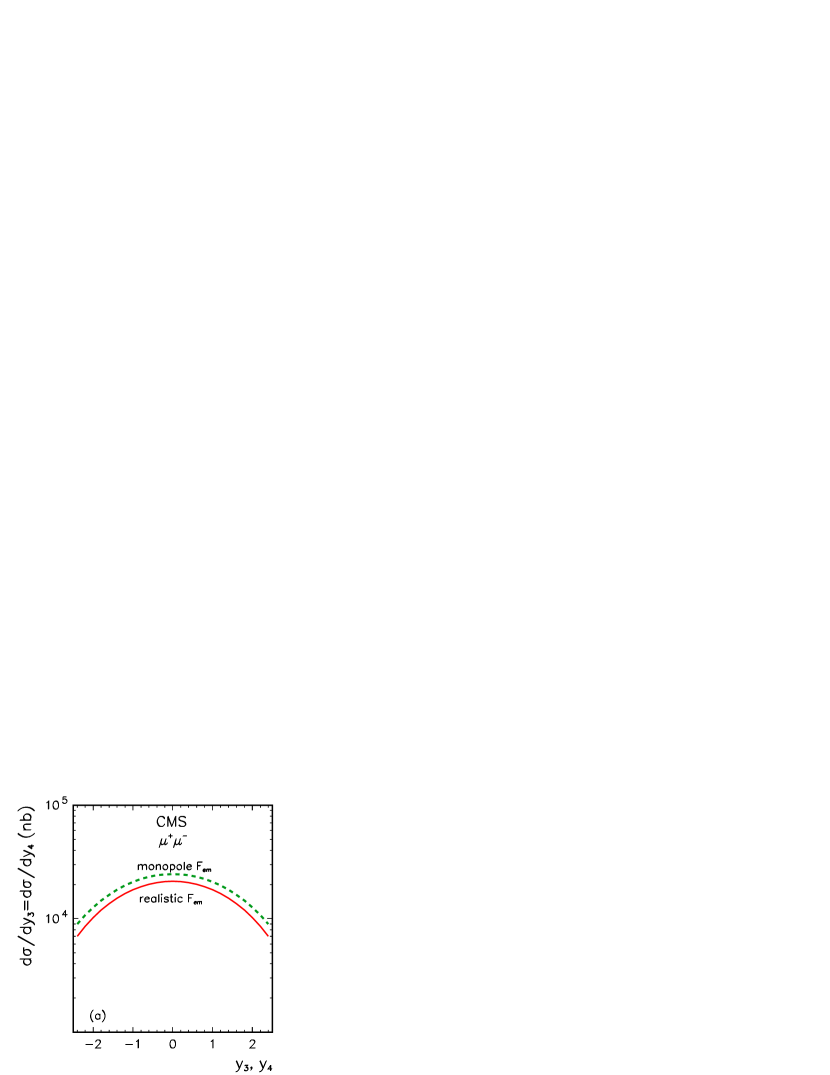
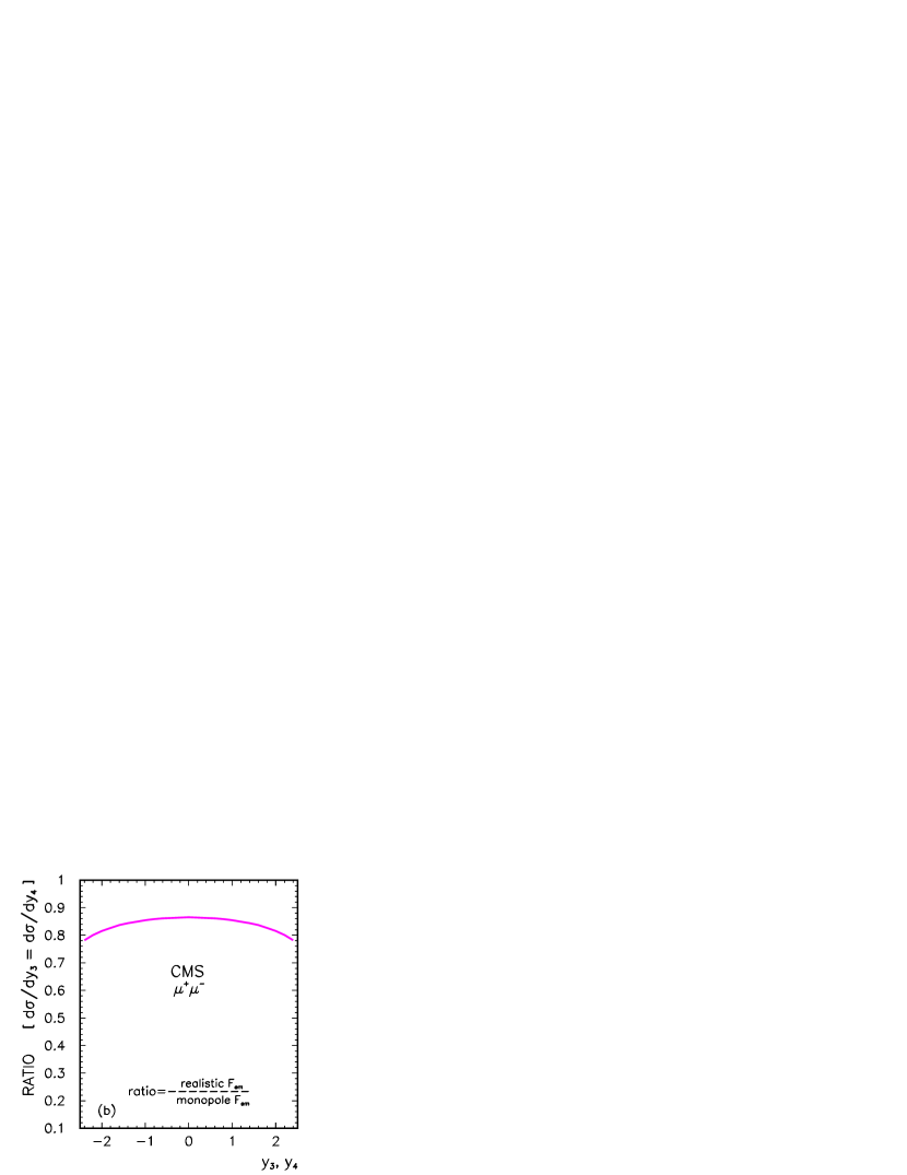
The cross section dependence on the muon rapidity is shown in Fig.24. Rather large cross section of the order of 0.1 mb is expected within the CMS acceptance. The average deviation with respect to the monopole form factor is about 20% (see the left panel).

Refer to caption
Refer to caption
Figure 24: (Color online) The muon rapidity distribution $\frac{{\rm d}\sigma}{{\rm d}y_{3}}$ (left) and the ratio (right) for the CMS conditions: $y_{3},y_{4}\in(-2.5,2.5)$, $p_{3t},p_{4t}\geq$ 4 GeV and $W_{NN}=5.5$ TeV.

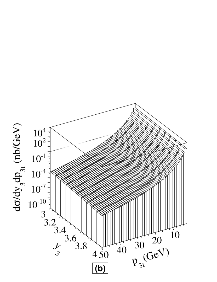
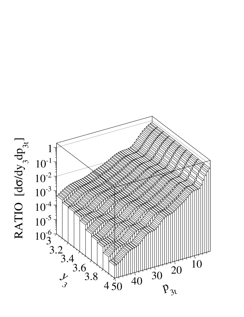
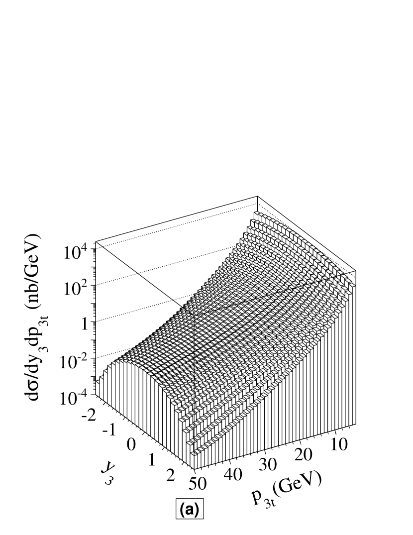
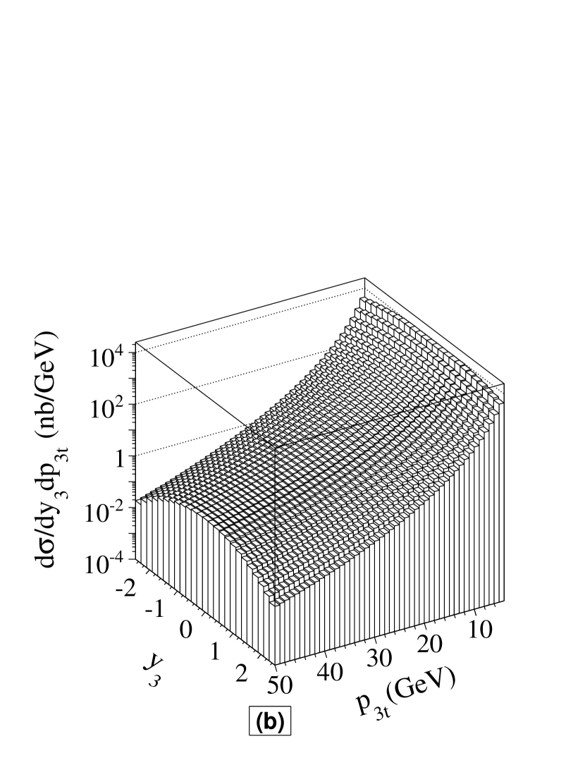
The two-dimensional distributions within the main CMS detector are shown in Fig.25. Big modifications with respect to the monopole case can be seen for large $p_{t}$ and $\left|y_{\mu^{+}},y_{\mu^{-}}\right|\sim$ 2.5, which is also presented in the form of the ratio in Fig.26.

Refer to caption
Refer to caption
Figure 25: $\frac{{\rm d}\sigma}{{\rm d}y_{3}\,{\rm d}p_{3t}}$ for realistic (left) and monopole (right) form factors for the CMS conditions: $y_{3},y_{4}\in(-2,5.2,5)$, $p_{3t},p_{4t}\geq$ 4 GeV and $W_{NN}=5.5$ TeV.
Refer to caption
Figure 26: The ratio of the realistic and monopole cross sections $\frac{{\rm d}\sigma}{{\rm d}y_{3}\,{\rm d}p_{3t}}$ for the CMS conditions: $y_{3},y_{4}\in(-2.5,2.5)$, $p_{3t},p_{4t}\geq$ 4 GeV and $W_{NN}=5.5$ TeV.

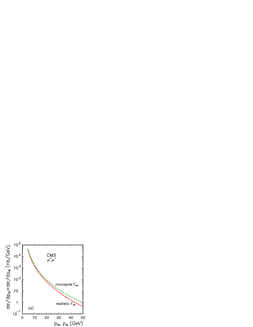
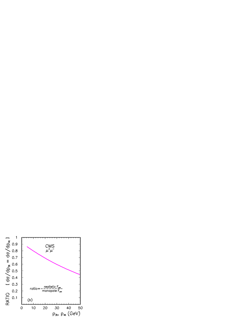
Finally, for completeness in Fig.27 we show the distributions in the $(y_{3},y_{4})$ plane. Here the distributions obtained with the monopole and realistic form factors are rather similar, but one should realize that these distributions are dominated by muons with small transverse momenta that are only slightly bigger than the experimental acceptance $p_{t}>2.5$ GeV and as a consequence relatively small $t_{1}$ and $t_{2}$ values.

Refer to caption
Refer to caption
Figure 27: $\frac{{\rm d}\sigma}{{\rm d}y_{3}\,{\rm d}y_{4}}$ for realistic (left) and monopole (right) form factors for the CMS conditions: $y_{3},y_{4}\in(-2.5,2.5)$, $p_{3t},p_{4t}\geq$ 4 GeV and $W_{NN}=5.5$ TeV.

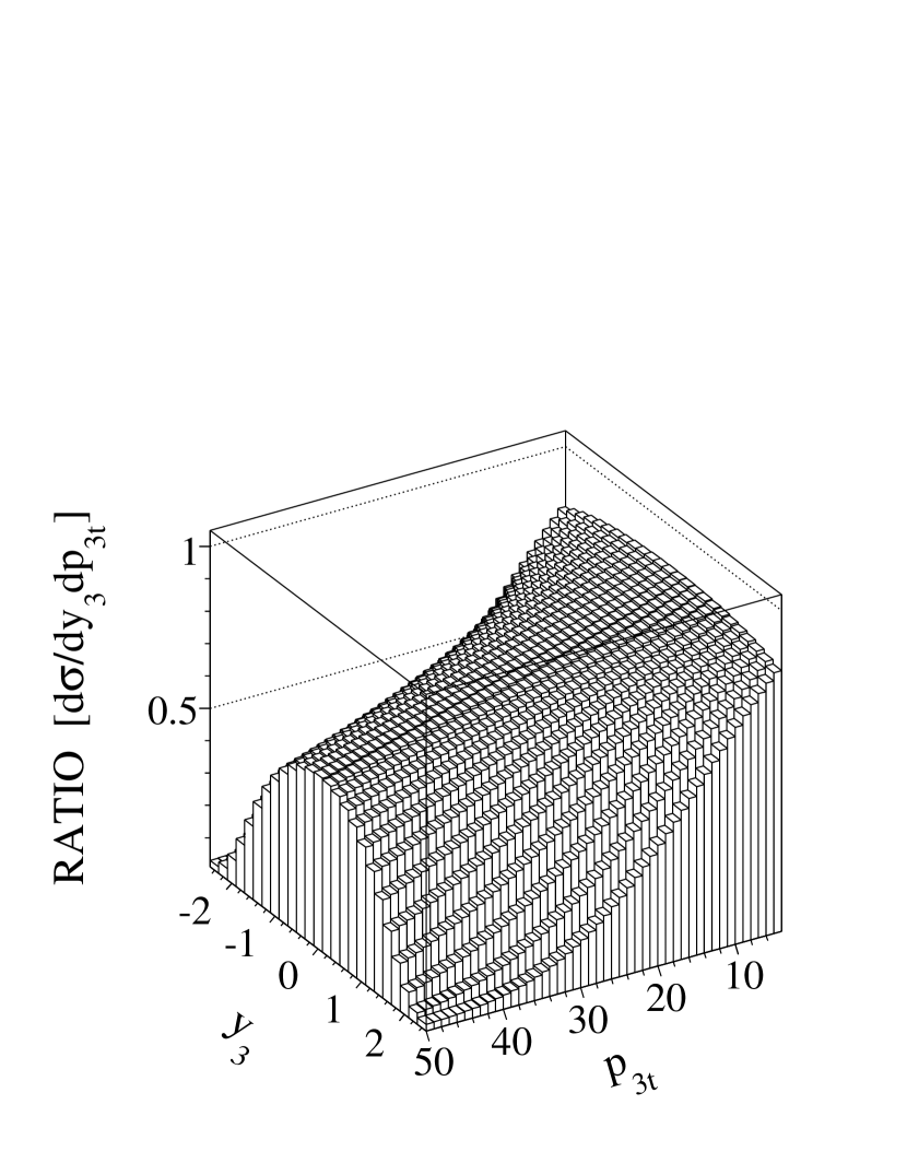
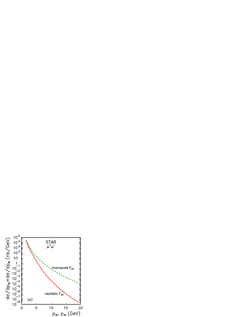
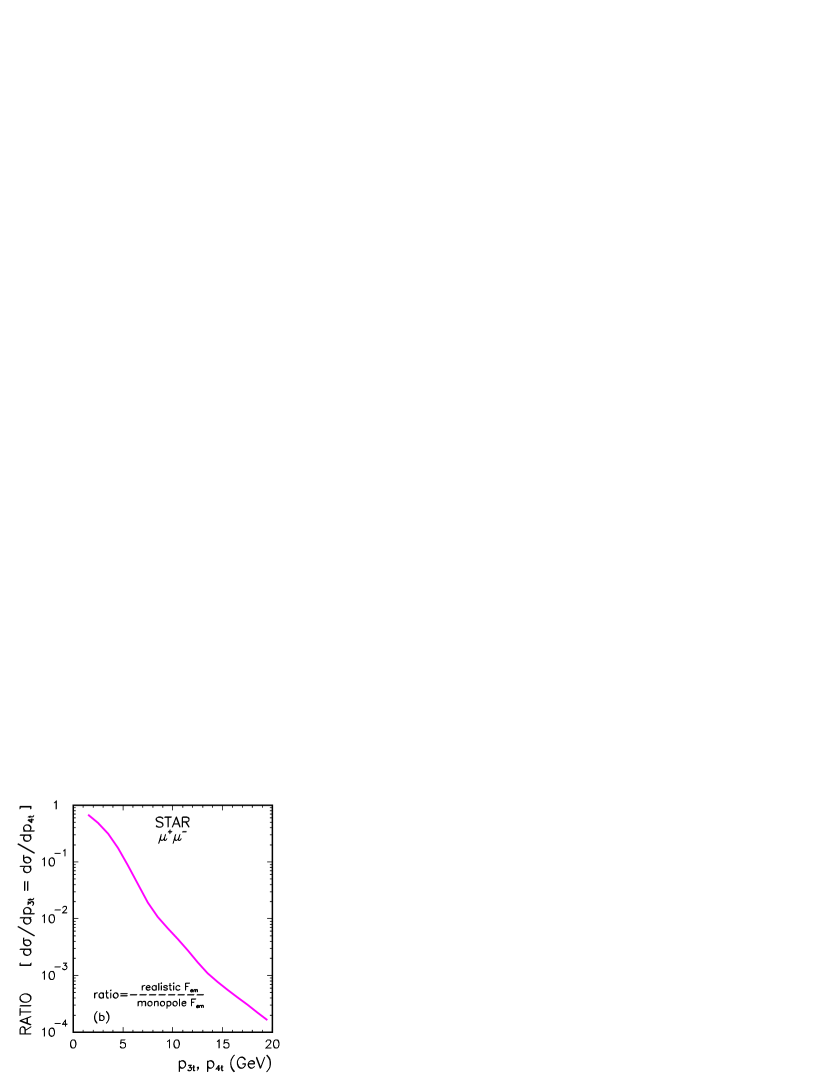
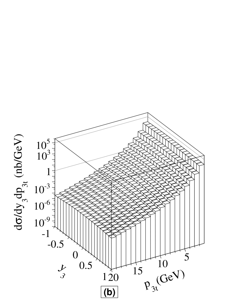
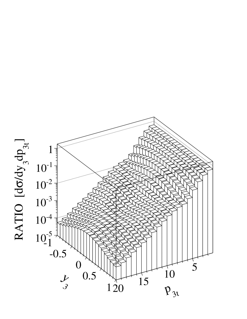
The same processes can be also studied at the being presently in the operation RHIC. Here STAR and PHENIX detectors can be used. The distribution of the muon transverse momentum is shown in Fig.28. The STAR rapidity cuts -1 $<y_{3},y_{4}<$ 1 are taken into account. Compared to the LHC the transverse momentum distributions decrease much faster. This fast fall-off limits the real measurements to relatively small transverse momenta of the order of 10 GeV. The inclusion of realistic charge distribution is here much more important than for the CMS conditions. The relative effect of damping with respect to the results with the monopole charge form factor is shown in the right panel. At $p_{t}$ = 10 GeV the damping factor is as big as 100! Experiments at RHIC have a potential to confirm this prediction.

Refer to caption
Refer to caption
Figure 28: (Color online) $\frac{{\rm d}\sigma}{{\rm d}p_{3t}}$ (left) and the ratio (right) for the STAR conditions: $y_{3},y_{4}\in(-1,1)$, $p_{3t},p_{4t}\geq$ 1 GeV and $W_{NN}=200$ GeV.

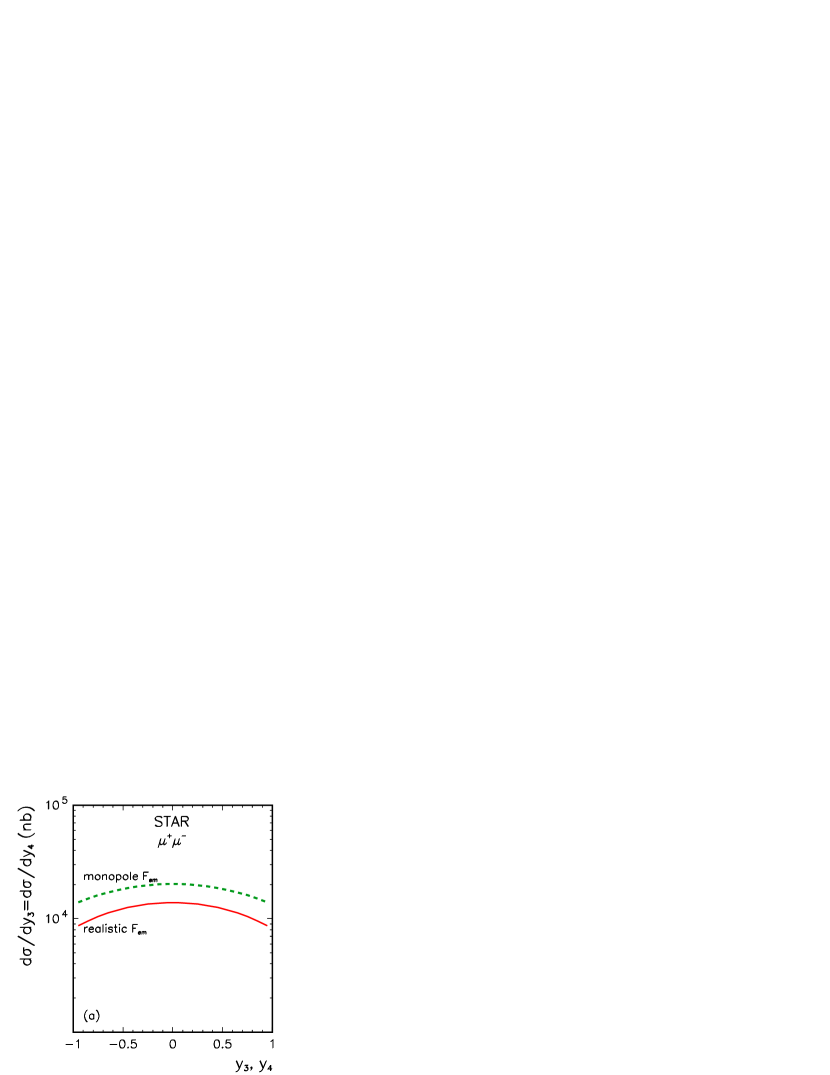
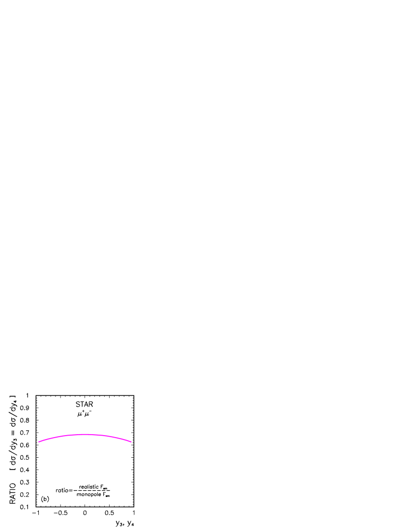
In general, one could also inspect the rapidity distributions. Our predictions are shown in Fig.29. We predict the 30-40 % cross section damping with respect to the reference calculation (monopole charge form factor).

Refer to caption
Refer to caption
Figure 29: (Color online) $\frac{{\rm d}\sigma}{{\rm d}y_{3}}$ (left) and the ratio (right) for the STAR conditions: $y_{3},y_{4}\in(-1,1)$, $p_{3t},p_{4t}\geq$ 1 GeV and $W_{NN}=200$ GeV.

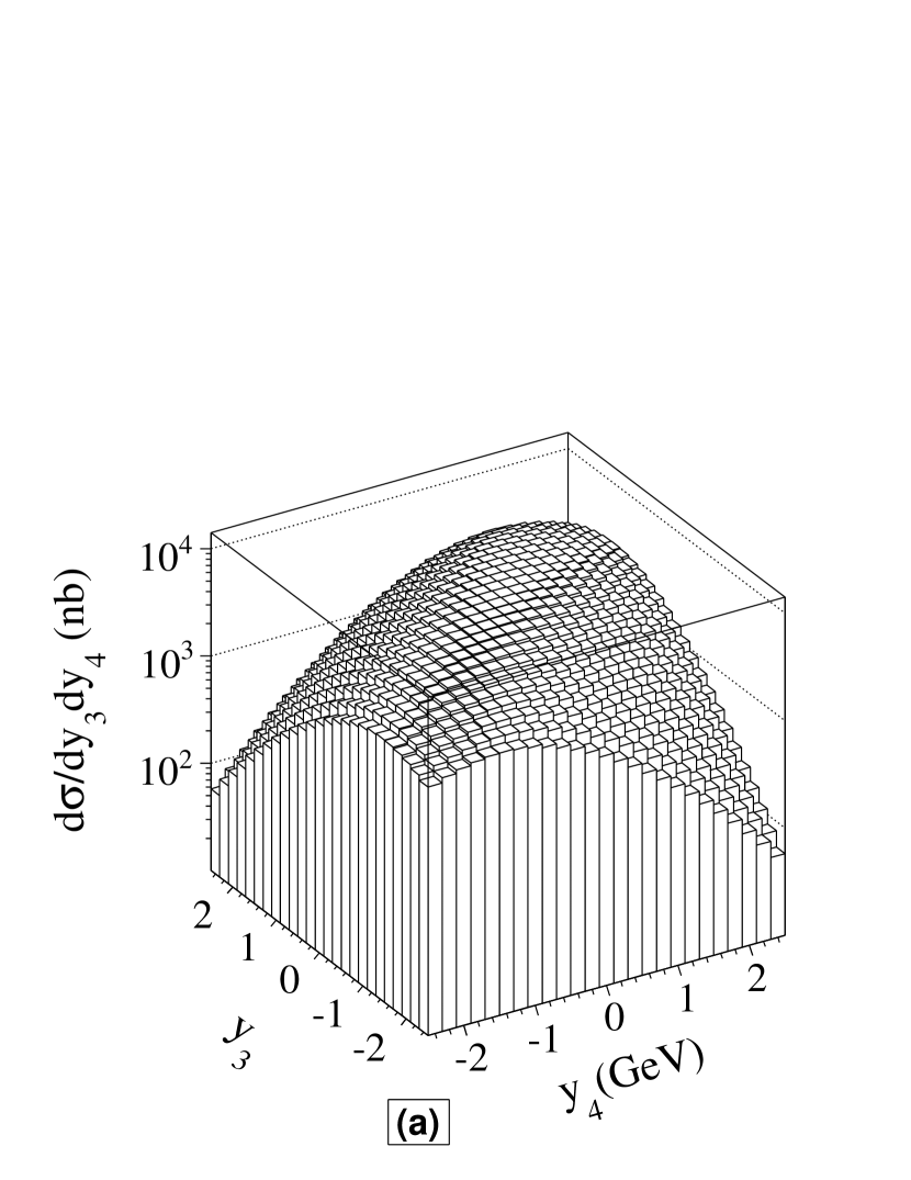
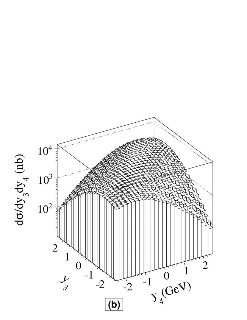
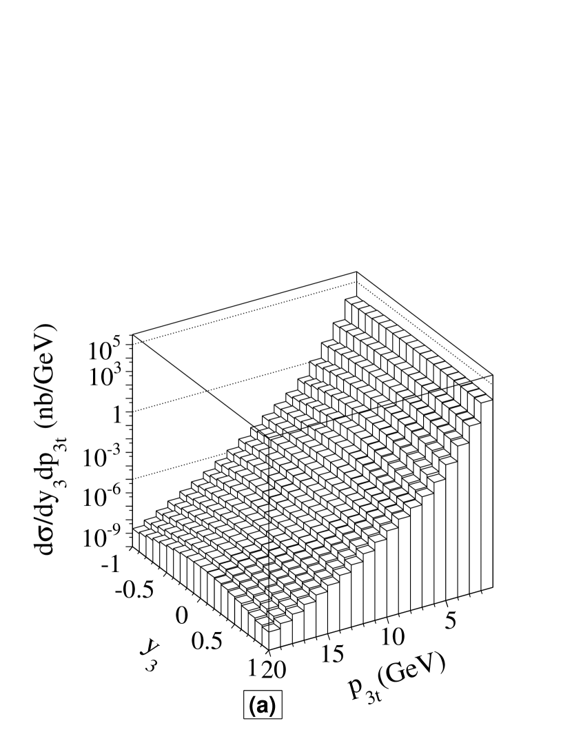
The two-dimensional distributions in muon rapidity and muon transverse momenta are shown in Fig.30 for the realistic and monopole form factors. Their ratio is presented in Fig.31. Again as for the transverse momentum distribution (see Fig.28) a huge damping can be observed. The irregular structure of the ratio reflects the strong nonmonotonic dependence of the charge form factors of $Au$ nuclei on $t_{1}$ and $t_{2}$. For completeness in Fig.32 we show the distribution of the dimuon invariant mass. The effect of the form factor oscillations shows up at large dimuon invariant masses where the ”realistic” cross section is rather small.

Refer to caption
Refer to caption
Figure 30: $\frac{{\rm d}\sigma}{{\rm d}y_{3}\,{\rm d}p_{3t}}$ for realistic (left) and monopole (right) form factor for the STAR conditions $y_{3},y_{4}\in(-1,1)$, $p_{3t},p_{4t}\geq 1$ GeV and $W_{NN}=200$ GeV.
Refer to caption
Figure 31: The ratio of the two-dimensional distributions from the previous figure for the STAR conditions: $y_{3},y_{4}\in(-1,1)$, $p_{3t},p_{4t}\geq 1$ GeV and $W_{NN}=200$ GeV.
Refer to caption
Figure 32: (Color online) Invariant mass distribution $\frac{{\rm d}\sigma}{{\rm d}M_{\mu^{+}\mu^{-}}}$ for the STAR conditions: $y_{3},y_{4}\in(-1,1)$, $p_{3t},p_{4t}\geq 1$ GeV and $W_{NN}=200$ GeV.

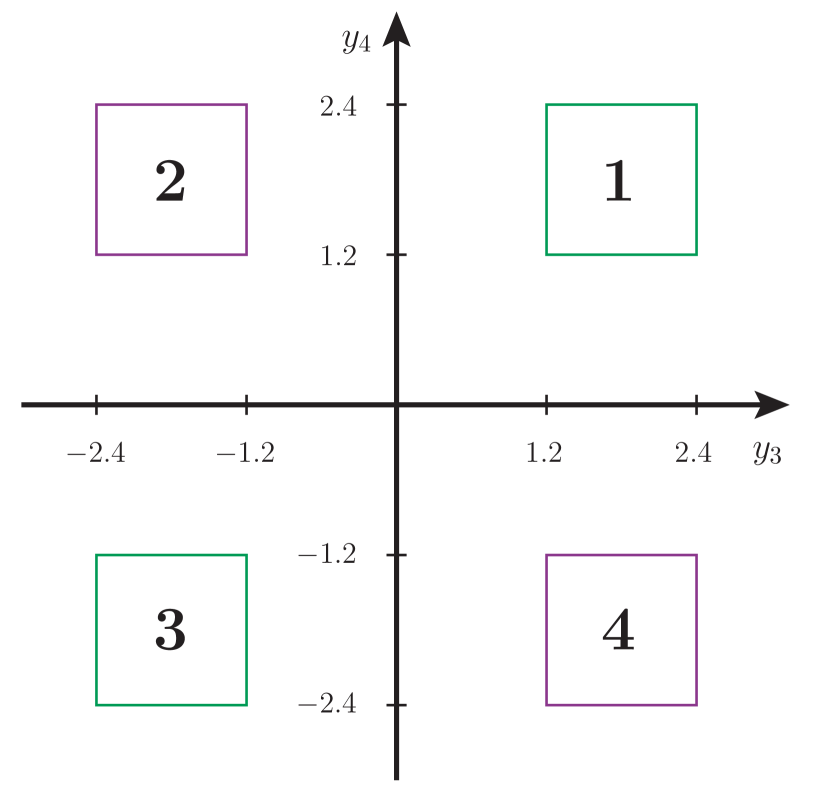
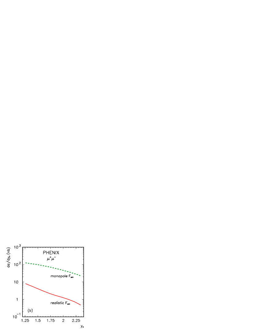
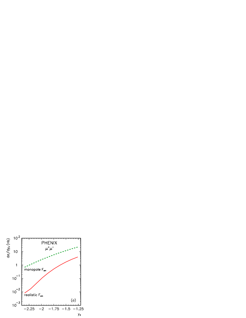
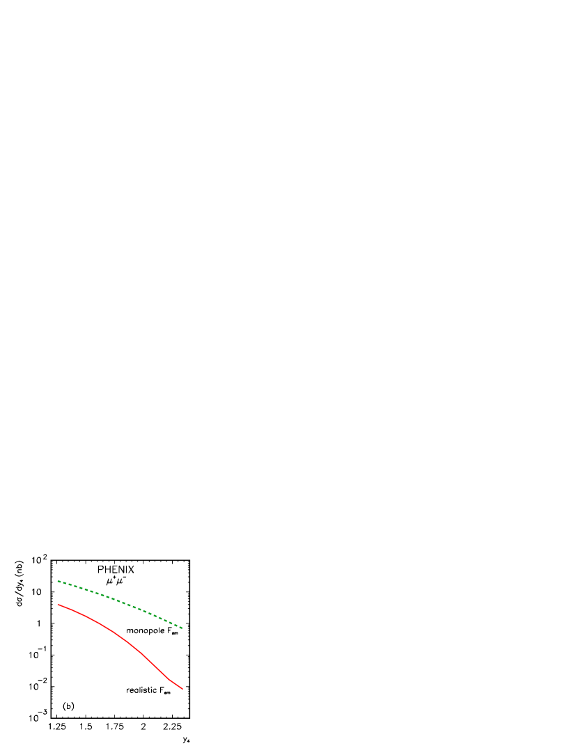
The PHENIX collaboration can measure muons in a rather limited range of rapidities shown in Fig.33. We have given names to the four possible regions (squares) in the figure. In spite of these limitations, still interesting measurements can be done. As an example in Fig.34 and Fig.35 we show our predictions for SQUARE1 and SQUARE2, respectively (the results for SQUARE3 and SQUARE4 are not shown as can be obtained by symmetry). Again large deviations from the monopole form factor results are predicted.

Refer to caption
Figure 33: (Color online) The muon rapidity regions available by the PHENIX detector.
Refer to caption
Refer to caption
Figure 34: (Color online) SQUARE 1: $\frac{{\rm d}\sigma}{{\rm d}y_{3}}$ (left) and $\frac{{\rm d}\sigma}{{\rm d}y_{4}}$ (right) for the PHENIX conditions: 1.2 $<|y_{3},y_{4}|<$ 2.4, $p_{3t},p_{4t}\geq$ 2 GeV and $W_{NN}=200$ GeV.
Refer to caption
Refer to caption
Figure 35: (Color online) SQUARE 2: $\frac{{\rm d}\sigma}{{\rm d}y_{3}}$ (left) and $\frac{{\rm d}\sigma}{{\rm d}y_{4}}$ (right) for the PHENIX conditions: 1.2 $<|y_{3},y_{4}|<$ 2.4, $p_{3t},p_{4t}\geq$ 2 GeV and $W_{NN}=200$ GeV.

IV Conclusions

The production of charge leptons in heavy ion collisions was proposed recently as a ”laboratory” for studying Quantum Electrodynamics effects, in particular the multiple photon exchanges. While very interesting theoretically it is still nonrealistic because of other approximations made in the calculations.

In this paper we have presented a study of the role of charge density for the differential distributions of muons produced in exclusive ultra-peripheral production in ultrarelativistic heavy ion collisions. Most of the calculations in the literature use so-called monopole charge form factor, which allows to write several formulae analytically. While it may be reasonable for the total rate of the dimuon production it is certainly too crude for differential distributions and for the cross sections with extra cuts imposed on transverse momenta of muons.

We have performed calculations in the Equivalent Photon Approximation in the impact parameter space and in the momentum space using Feynman diagrammatic approach. The first method is very convenient to include absorption effects, while the second one allows to study differential distributions.

Our calculations show that the results obtained with the realistic and the approximate form factors can differ considerably, in some parts of the phase space even by orders of magnitude. The effects related to the charge distribution in nuclei are particularly important at large rapidities of muons and at large transverse momenta of muons.

We have also discussed the role of absorption effects which can be easily estimated in the impact parameter space. This allows to estimate the absorption effects for the total rate or for the rapidity distribution of the dimuon pairs. Estimating this effect in the case of differential distributions is not simple, but could be studied in the future.

We have presented predictions for the STAR and PHENIX detectors at RHIC as well as for the ALICE and CMS detectors at LHC. In all cases we have found significant deviations from the reference calculation for the monopole form factor. It would be interesting to pin down the effects discussed here and verify the present predictions in future studies at LHC. Both ALICE and CMS detectors could be used in such studies.

In practice such studies may not be simple as an efficient trigger for the peripheral collisions is required. The multiphoton exchanges leading to additional excitation of nuclei and subsequent emission of neutrons could be useful in this context (see e.g. BGKN09 ). The neutrons could be then measured by the Zero Degree Calorimeters. First measurements of this type for $e^{+}e^{-}$ pair emission have been already performed by the STAR and PHENIX collaborations STAR ; PHENIX .

In the present calculation we have restricted to lowest-order QED calculations paying a special attention to realistic form factors and absorption effects and totally ignored higher-order corrections. How important are the QED higher-order correction was demonstrated recently in Refs.Baltz2 ; SB . While Jentschura and Serbo SB argue that the higher-order corrections are rather small, Baltz Baltz2 finds a huge reduction of the integrated cross section of the order of 20%. Cleary the discrepancy should be clarified in the future. It would be also very interesting to calculate the higher-order corrections for differential distributions which will be measured at LHC 222All LHC experiments: ATLAS, CMS and ALICE, will impose severe cuts on transverse momenta and pseudorapidities of charged leptons.. The latter calculations seem to us rather difficult technically.

In the moment it seems precocious to answer the question whether the processes discussed here could be used as a luminosity monitor for heavy ion collisions at LHC. In our opinion, first these processes should be measured and compared to theoretical calculations. In addition, the influence of the absorption effects and multiphoton processes on differential distributions should be studied in more detail.

Acknowledgments

The discussion with Janusz Chwastowski, Jacek Okołowicz, Wolfgang Schäfer and Valeryi Serbo is acknowledged. This work was partially supported by the Polish grant N N202 078735.

References

  • (1) V.M. Budnev et.al, Phys. Rep. 15 (1975) 4.
  • (2) G. Baur, K. Hencken, D. Trautmann, S. Sadovsky and Y. Kharlov, Phys. Rep. 364 (2002) 359.
  • (3) A. Baltz et al., Phys. Rep. 458 (2008) 1.
  • (4) E. Bartos, S.R. Gevorkyan, N.N. Nikolaev and E.A. Kuraev, Phys. Rev. A66 (2002) 042720; E. Bartos, S.R. Gevorkyan, E.A. Kuraev and N.N. Nikolaev, J. Exp. Theor. Phys. 100 (2005) 645.
  • (5) D.Yu. Ivanov, A. Schiller and V.G. Serbo, Phys. Lett. B454 (1999) 155;
    K. Henecken, E.A. Kuraev and V.G. Serbo, Phys. Rev. C75 (2007) 034903;
    U.D. Jentschura, K. Hencken and V.G. Serbo, Eur. Phys. J. C58 (2008) 281;
    U.D. Jentschura and V.G. Serbo, Eur. Phys. J. C64 (2009) 309.
  • (6) A. Baltz, Phys. Rev. Lett. 100 (2008) 062302.
  • (7) A. Baltz, Phys. Rev. C80 (2009) 034901.
  • (8) M. Kłusek, A. Szczurek, W. Schäfer, Phys. Lett. B674 (2009) 92.
  • (9) R.C. Barrett and D.F. Jackson, ”Nuclear Sizes and Structure”, Clarendon Press, Oxford 1977.
  • (10) H. de Vries, C.W. de Jager and C. de Vries, Atomic Data and Nuclear Data Tables, 36 (1987) 495.
  • (11) K. Hencken, D. Trautmann and G. Baur, Phys. Rev. A49 (1994) 1584.
  • (12) J.D. Jackson, Classical Electrodynamics, 2nd ed. (Wiley, New York, 1975), p. 722.
  • (13) G. Baur and L.G. Ferreiro Filho, Phys. Lett. B254 (1991) 30.
  • (14) U.D. Jentschura, V.G. Serbo, Eur. Phys. J. C64 (2009) 309.
  • (15) A.J. Baltz, Y. Gorbunov, S.R. Klein and J. Nystrand, Phys. Rev. C80 (2009) 044902.
  • (16) J. Adams et al. (STAR collaboration), Phys. Rev. C70 (2004) 031902(R).
  • (17) S. Afanasiev et al. (PHENIX collaboration), Phys. Lett. B679 (2009) 321.