CERN-PH-TH/2010-092
LAPTH-017-10
Dark energy with non-adiabatic sound speed:
initial conditions and detectability
Guillermo Ballesteros111ballesteros@pd.infn.it
Museo Storico della Fisica e Centro Studi e Ricerche “Enrico Fermi”.
Piazza del Viminale 1, I-00184, Rome.
Dipartimento di Fisica “G. Galilei”, Università degli Studi di Padova, via Marzolo
8, I-35131 Padova, Italy.
INFN, Sezione di Padova, via Marzolo 8, I-35131 Padua, Italy.
Julien Lesgourgues222julien.lesgourgues@cern.ch
CERN, Theory Division, CH-1211 Geneva 23, Switzerland.
Institut de Théorie des Phénomènes Physiques, EPFL, CH-1015 Lausanne,
Switzerland.
LAPTh (CNRS - Université de Savoie), BP 110, F-74941 Annecy-le-Vieux
Cedex, France.
Abstract
Assuming that the universe contains a dark energy fluid with a constant linear equation of state and a constant sound speed, we study the prospects of detecting dark energy perturbations using CMB data from Planck, cross-correlated with galaxy distribution maps from a survey like LSST. We update previous estimates by carrying a full exploration of the mock data likelihood for key fiducial models. We find that it will only be possible to exclude values of the sound speed very close to zero, while Planck data alone is not powerful enough for achieving any detection, even with lensing extraction. We also discuss the issue of initial conditions for dark energy perturbations in the radiation and matter epochs, generalizing the usual adiabatic conditions to include the sound speed effect. However, for most purposes, the existence of attractor solutions renders the perturbation evolution nearly independent of these initial conditions.
1 Introduction
The biggest problem in cosmology today is the understanding of the accelerated expansion of the universe. Although one could try to attack this question leaving aside the cosmological principle or modifying Einstein’s gravity, the most classical approach consists of assuming a perturbed FLRW universe with a negative pressure component. The minimal model (in terms of number of free parameters) compatible with the current data is a cosmological constant, which should be perfectly homogeneous by definition. Other candidates (which may or may not alleviate the fine–tuning and coincidence problems of the cosmological constant) include, for instance, scalar field models, or effective descriptions in terms of a fluid with free parameters yet to be measured. A canonically kinetic normalized scalar field would fluctuate, but since in that case the sound speed (computed in the rest frame of the scalar field) is equal to one, local pressure would prevent density contrasts to grow significantly. In an effective fluid description, the sound speed is a free parameter, and dark energy clustering can be more efficient in the limit in which overdensities are not balanced by local pressure perturbations () .
Generally speaking, the study of small perturbations could be used as a tool for discriminating between various models with a negative pressure component (cosmological constant, dark energy fluid, quintessence or k–essence fields, coupled dark energy, etc.) or a modified theory of gravity. One of the major difficulties comes from the fact that the expansion history predicted by a given Lagrangian theory of gravity can be reproduced in General Relativity by a dark fluid having an appropriate (time varying) equation of state, or by a scalar field with an adequate kinetic term and potential. Fortunately, a very precise measurement of clustering properties in our universe could at least help to discard some models in favor of others at the level of perturbations [1, 2]. However, the spatial fluctuations of typical dark energy models are very much suppressed with respect to those of dark matter, and detecting their effect is a real challenge.
The effects of quintessence perturbations (for which ) on the CMB and LSS power spectra were discussed in [3]. For an (uncoupled) dark energy fluid, there have been several studies on the possibility to measure , but its value remains unconstrained with present data (see e.g. [4, 5, 6, 7, 8, 9, 10, 11]). In a recent attempt, the authors of [10] used present Cosmic Microwave Background (CMB), Large Scale Structure (LSS) and supernovae data (including CMBLSS cross–correlation), and showed that it is possible to see some weak preference for , but only for a certain kind of early dark energy model in which the equation of state is not constant. We may still hope to discriminate between different values of using combinations of future CMB data with 3–dimensional galaxy clustering data [12], with CMBLSS cross–correlation data [13], or with results from a large neutral hydrogen survey such as that of the SKA project [14] (see also [15]).
In this work, we focus on an effective description which has already been studied by several authors: namely, a dark energy fluid with a linear equation of state , a constant equation of state parameter close to and a constant sound speed defined in the range . In Section 2 we review the concept of sound speed for a cosmological fluid. The purpose of Section 3 is to clarify the non-trivial issue of initial conditions for dark energy perturbations in the radiation era, which are a priori non–adiabatic since . We present for the first time the initial conditions fulfilled by the dark energy fluid in the synchronous gauge (i.e., in the gauge used by most Boltzmann codes), when all other fluids have adiabatic primordial perturbations. In Section 4 we study analytically the evolution of these perturbations during the matter epoch. We derive approximations for the attractor solutions followed by dark energy perturbations (both in the Newtonian and synchronous gauges). These new results can be used in the future for analytical estimates of the impact of dark energy on structure formation. In Section 5, in order to update the analysis of [13], we carry a full Monte-Carlo exploration of the likelihood of future mock CMB and LSS data, in order to infer the sensitivity of these data to the dark energy sound speed, and to investigate possible parameter degeneracies. Finally, in Section 6, we summarize our findings.
2 The sound speed
At the level of inhomogeneities, the sound speed of a cosmological fluid plays a similar role to that of the equation of state for the background cosmology, and relates the pressure and density perturbations as:
| (2.1) |
Defined in this way, the sound speed is gauge dependent. Indeed, the quantity that can be assumed to be a definite number (depending on the microscopic properties of the fluid) is the ratio evaluated in the fluid rest frame, often denoted as . In another arbitrary frame, gets corrections related to the velocity of the fluid in that frame, such that in Fourier space [4]
| (2.2) |
where is the relative density perturbation, the velocity divergence of the fluid, the comoving wavenumber, the conformal Hubble parameter , and the adiabatic sound speed of the fluid. The latter is defined as the (time dependent) proportionality coefficient between the time variations of the background pressure and energy density of the fluid,
| (2.3) |
For non–interacting fluids one finds that
| (2.4) |
which implies that if is constant and different from . In the rest of this work, we will focus on the case in which can indeed be approximated as a constant in time. Besides, we will restrict our analysis to . The lower bound prevents dark energy fluctuations from growing exponentially, which can lead to unphysical situations; and the upper one is imposed in order to avoid superluminal propagation. For a study on the implications of the sign and value of for quintessence see [16]. For an expression relating the time evolution of and through the intrinsic entropy contribution to the pressure perturbation see [33] (and also [34]).
3 Initial Conditions
In order to compute the CMB and LSS power spectra, one needs to evolve cosmological perturbations starting from initial conditions deep inside the radiation epoch and far outside the Hubble radius. Initial conditions for photons, neutrinos, cold dark matter and baryons are reviewed in [17] in the synchronous and Newtonian gauges (see also [18]). Here, we want to extend this set of relations to dark energy perturbations, especially in the gauge used by most Boltzmann codes: namely, the synchronous gauge. Surprinsingly, this issue has been overlooked in the literature, without a clear justification333There were however various studies closely related to this issue. For instance, in [19] various possible initial conditions for the quintessence field, and their impact on the CMB were discussed. In [20], the initial conditions for a dark energy fluid with quintessence-like perturbations were obtained in a gauge invariant formalism. In [21], the technique of [20] was extended to interacting dark energy models. In all these works, the dark energy sound speed was kept fixed to one.. In practical terms, initial conditions for dark energy perturbations are essentially irrelevant for most purposes because of the existence of an attractor. We wish to clarify this issue and write down explicitly this attractor solution.
Adiabatic initial conditions on super–Hubble scale derive from the generic assumption that for each component , the density can be written as , where stands for the background density, and is an initial time–shift function independent of . Similarly the pressure would read . Such conditions can be easily justified in all models in which primordial perturbations are generated from a single degree of freedom (like the inflaton), and/or in cases in which all components have been in thermal equilibrium in the early universe with a common temperature and no chemical potential. This form implies
| (3.1) | |||||
| (3.2) |
and hence , i.e. the sound speed of each species must be equal to its adiabatic sound speed. This generic assumption also implies that the total ratio is independent of the purely spatial coordinates . Finally, if all the components do not interact, we conclude that
| (3.3) |
The fact that for all species the ratios are equal to each other is a well-known property of adiabatic initial conditions. The meaning of such a relation is not so clear when one introduces a dark energy fluid, for which . Hence, in most frames, one has and the fluid cannot obey simultaneously (3.1) and (3.2). This raises the issue of defining sensible initial conditions for a dark energy fluid. However, during radiation and matter domination, dark energy perturbations tend to fall inside the gravitational potential wells created by the dominant component and not much concern has been raised concerning their initial conditions. In other words, there is an attractor solution for dark energy perturbations, and their initial values are almost irrelevant in practice, provided that for each Fourier mode the attractor is reached before dark energy comes to dominate (i.e. provided that initial conditions are imposed early enough, and that initial dark energy perturbations are not set to dramatically large values). For this reason, in a Boltzmann code like camb [22], initial dark energy perturbations are set by default to zero.
We will derive in the next subsections the attractor solution for a dark fluid with constant and arbitrary , assuming that other quantitites obey the usual adiabatic initial conditions, and in two gauges: the Newtonian and the synchronous ones. For a detailed account of the construction of the two gauges and the relations among them we refer the reader to [17] . In what follows, we will denote quantities corresponding to the conformal Newtonian gauge with a superscript. For instance, denotes the relative dark energy density in that gauge. No superscript will be used for quantities in the synchronous gauge. The transformation equations between the two gauges will be summarized below, later in this section.
3.1 Synchronous gauge
Early in the radiation era, the total energy density of the universe can be approximated by the sum of photon and neutrino densities, with a constant ratio . In order to find the perturbation evolution on super-Hubble scales and for adiabatic initial conditions, one can combine the Einstein, photon and neutrino equations into a fourth order linear differential equation for the trace part of the metric perturbations in Fourier space [17]. The fastest growing mode among the four possible solutions, , corresponds to the growing adiabatic mode.
Since these conditions are established when the perturbations are still in the super–Hubble regime, the product can be used as an expansion parameter for the solutions of the dynamical equations. At leading order
| (3.4) |
where the subscripts refer to cold dark matter, baryons, neutrinos and photons; and is a constant. As usual, in order to fully fix the gauge, we impose not only synchronous metric perturbations, but also that dark matter particles have a vanishing velocity divergence . The continuity and Euler equations for the dark energy fluid read
| (3.5) | |||||
| (3.6) |
These equations are very general, since the only underlying assumption is that the fluid is non–interacting, and allow for the presence of shear stress , non–adiabatic sound speed, and a time varying . From now on we assume that the fluid is shear free and has a constant equation of state. If the energy density of dark energy at early times is negligible, the solution for the metric perturbation will not change. In order to find the attractor solution, we just need to replace in (3.5) according to (3.4), and solve equations (3.5), (3.6). As expected, we find that the solution of the homogeneous equation becomes negligible with time, while and are driven to
| (3.7) | |||||
| (3.8) |
at lowest order in .
This attractor solution does not look like usual adiabatic initial conditions because, in general, is different from in the synchronous gauge. Hence, cannot be equal to . However, this solution gives the correct behavior of dark energy perturbations when the other components obey adiabatic initial conditions, once the attractor has been reached. Therefore they could be called “generalized initial adiabatic conditions”. These conditions are valid not only for dark energy fluids () but also for any other fluid with constant and . For instance, one can easily check that the usual adiabatic initial conditions for matter and radiation can be recovered from (3.7, 3.8) by choosing .
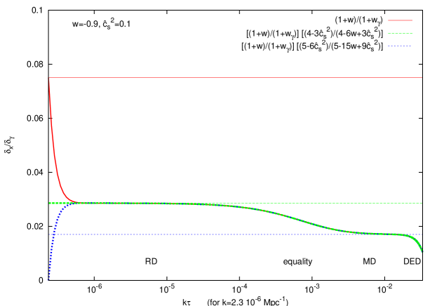
In a Boltzmann code like camb [22], the quantitites and are fixed to zero at initial time for simplicity. For most practical applications, this arbitrary choice does not introduce any mistake in the final results, since and are quickly driven to the attractor solutions of eqs. (3.7, 3.8). We illustrate this in Figure 1, for a very large wavelength mode. We suggest however to implement eqs. (3.7, 3.8) directly into camb’s initial condition routine (as we did in Section 5 of this work), since this is completely straightforward, and since it offers a guarantee that final results are independent of the early time at which initial conditions are defined.
3.2 Conformal Newtonian Gauge
The equations that give the evolution of a generic fluid in the conformal Newtonian gauge are (see also [10])
| (3.9) | |||||
| (3.10) |
The metric perturbations
| (3.11) | |||||
| (3.12) |
can be obtained from those of the synchronous gauge using
| (3.13) |
where is the traceless part of the metric scalar perturbation in the synchronous gauge in Fourier space. Using these last equations one can immediately check that the product has zero time derivative, so that and are time independent at lowest order in . One can either solve directly (3.9, 3.10), or use our results (3.7, 3.8) for the behavior of and in the synchronous gauge, and perform the gauge transformations
| (3.14) | |||||
| (3.15) | |||||
| (3.16) |
that are valid for non–interacting fluids. The two methods give
| (3.17) | |||||
| (3.18) |
where
| (3.19) |
and
| (3.20) |
Notice that the leading contributions to the velocity and density perturbations in the conformal Newtonian gauge are independent of the speed of sound and such that
| (3.21) |
Therefore, the usual adiabatic conditions are recovered, and enters only in the next order corrections444 Note that the gauge transformation law (3.14) implies that (3.22) for any fluid with constant equation of state . Since the usual adiabatic conditions hold at leading order in the Newtonian gauge, one may naively infer from the above equality that they hold also in the synchronous gauge. This is not correct since on the left-hand side, the two terms are dominated by order zero terms in a expansion, while on the right-hand side the leading terms are of order two. Assuming that the fluid has an adiabatic sound speed (like cold dark matter or photons), a full order-two calculation of all the terms leads to (3.23) The righ-hand side does not vanish since is by assumption strictly positive. Being of order two, this difference contributes to the solutions at leading order in the synchronous gauge, but only at next-to-leading order in the Newtonian gauge.. Indeed, the Newtonian gauge is the one in which, beyond the Hubble scale, is equal to at leading order, even when . This can be checked by keeping the dominant terms in (3.14, 3.15), and replacing and by these values in (2.2): one gets . So, in the Newtonian gauge and on super-horizon scale, is equal to for any fluid with contant , and the common intuition according to which super-Hubble fluctuations behave in the same way as background quantitites is recovered.
4 Late time attractors
In the previous section, we found the attractor solutions for dark energy perturbations during radiation domination. Here we will derive similar solutions during matter domination. These results can be used to provide initial conditions for dark energy perturbations in problems in which following the behavior of cosmological perturbations during radiation domination is not relevant.
If we assume that the energy density of photons and (massless) neutrinos is negligible deep inside matter domination, the perturbations can be studied using a two–fluid approximation. One of the fluids is formed by baryons and cold dark matter (which cannot be distinguished from each other) and the other one is dark energy. This description in terms of two components can be accurately used to study the growth of matter perturbations up to the present day. Mathematically, the problem consists of a system of six independent equations with six variables: the density and velocity perturbations of the two fluids plus the scalar metric perturbations. We will now find the relevant growing modes of the perturbations in the two gauges and conclude this section with some remarks concerning the initial conditions for dark energy.
4.1 Synchronous gauge
In the synchronous gauge, since we consider that cold dark matter and dark energy are shear free, the Einstein equations imply that the two metric degrees of freedom and are related to each other. Eliminating in terms of , and expressing in terms of (the continuity equation for cold dark matter gives ) , we obtain a system of two reasonably short second order differential equations that describe the evolution of density fluctuations [23] :
| (4.1) | |||||
| (4.2) | |||||
where
| (4.3) |
and
| (4.4) | |||||
| (4.5) |
In the purely matter dominated epoch (, ) the equation that describes the evolution of matter perturbations is the classical growth formula:
| (4.6) |
Its general solution is a linear combination of a growing mode and a decaying one . In order to find the relevant attractor solution for dark energy perturbations, one should keep the first of these two solutions
| (4.7) |
The behavior of cosmological perturbations depends on their wavelength as compared to the characteristic scales of the problem. In our case, and in terms of comoving scales, there are two relevant quantitites: the comoving Hubble scale (which gives the order of magnitude of the causal horizon associated to any process starting after inflation), and the comoving sound horizon . Analytical approximations for the evolution of dark energy perturbations can be obtained in the three regimes defined by these two scales.
For super–Hubble perturbations with , one can approximate (4.5) as , and the homogeneous part of (4.2) gives two decaying modes for . The growing solution, sourced by the dark matter perturbations, is
| (4.8) |
If instead , the perturbations are below the Hubble scale but above the sound horizon, and . As in the previous case, the growing mode for the density perturbations of dark energy comes from the one of dark matter:
| (4.9) |
These formulas agree with the results of [24] (when transformed into the synchronous gauge) if we take the sound speed to be zero. The equations (4.8) and (4.9) can be used to define initial conditions for a dark energy fluid during matter domination, provided that at the initial time all relevant wavelengths are still larger than the sound horizon. Below the sound horizon, it becomes more difficult to obtain simple analytic approximations. When , we can still approximate as in the previous case, but the term proportional to in (4.2) becomes dominant. One gets:
| (4.10) |
The general solution of the homogeneous equation goes as with a multiplicative factor that is a linear combination of the Bessel functions and . The particular solution for the complete equation including can also be written in terms of non–elementary functions. Dark energy perturbations are anyway suppressed with respect to dark matter ones in this regime, since below the sound horizon (i.e below the Jeans length of the fluid) the pressure perturbation can resist the gravitational infall. Indeed, equation (4.10) implies that in the limit , the dark energy density contrast should vanish.
4.2 Conformal Newtonian gauge
In the conformal Newtonian gauge, the complete equations for the evolution of density perturbations, equivalent to (4.1) and (4.2), become longer, because metric perturbations cannot be trivially replaced in terms of . Having obtained the solutions in the synchronous gauge, it is simpler to apply (3.14) rather than solving the conformal Newtonian equations directly. In the limit of pure matter domination, i.e. , one can easily prove that
| (4.11) |
and therefore
| (4.12) | |||||
| (4.13) |
These equations show that outside the Hubble radius, the solution is driven as usual to
| (4.14) |
The same equations also imply that in the regime , (4.9) remains valid in the conformal Newtonian gauge (relations valid inside the Hubble radius are expected to be gauge independent).
4.3 Attractor solutions
An important feature in the evolution of dark energy perturbations in the two gauges, which is common to the three regions we have studied, is that initial conditions for the dark energy perturbations are almost irrelevant for the evolution in the purely matter dominated epoch. During this period, dark energy fluctuations track matter inhomogeneities. Above the sound horizon, as soon as the attractor solution of (4.8) or (4.9) is reached, the ratio only depends on the sound speed and equation of state of the dark energy fluid. Notice that in the newtonian gauge the sound speed dependence actually disappears outside the Hubble scale.
In the dark energy dominated period (), the roles of the fluctuations are exchanged and matter perturbations are sourced by dark energy ones. However, since we have seen that it is only the initial value of that determines in the matter epoch, the initial conditions for the evolution in the dark energy period are in reality given only by . In accordance with the results of section 3 , this argument can be extended back into the radiation era. Besides, from the previous reasonings, it is clear that the velocity perturbations are also unimportant. In conclusion, the amount of dark energy perturbations today can be well estimated just by knowing the dark matter perturbations at some initial time in the radiation or the matter epoch. We illustrate this behavior in Figure 1 for a very large wavelength mode.
5 Detectability
The detectability of the sound speed of dark energy has already been studied by various authors, under different assumptions and for various datasets. For example, for a model with constant and (identical to the one we consider in this work), the authors of [10] showed that the combination of present CMB, LSS and supernovae data is not sensitive at all to the dark energy sound speed. Since dark energy perturbations would change the growth rate of matter inhomogeneities on intermediate scales (between the Hubble radius and the dark energy sound horizon), they can affect the CMB photon temperature through the Late Integrated Sachs-Wolfe (LISW) effect. Small variations in the LISW effect are difficult to detect in the CMB temperature spectrum, due to cosmic variance and to the fact that we only see the sum of primary anisotropies and LISW corrections. However, the LISW contribution can be separated from primary anisotropies by computing the statistical correlation between CMB and projected LSS maps of the sky. In [10], most of the presently available cross–correlation data were included in the analysis, but current statistical and systematic error bars are far too large for probing sub–dominant dark energy clustering effects.
One could think of constraining the dark energy sound speed in the future, either by measuring with better accuracy the auto–correlation function of matter distribution tracers (galaxy surveys, cluster surveys, lensing surveys, …) or, again, by studying their cross–correlation with CMB maps in order to extract the LISW contribution. The first option was studied for instance in [12], and the second in [13]. In the latter, the authors focus on the cross–correlation of a CMB experiment similar to Planck with a survey comparable to the Large Synoptic Survey Telescope (LSST) project. The author of [12] considered the combination of Planck with future galaxy redshift surveys, not including any cross–correlation information, but using the full three–dimensional power spectrum of galaxies instead of their angular power spectrum sampled in a few redshift bins (the loss of information on the LISW effect can then be compensated by more statistics on the auto-correlation function). Both works reached the same qualitative conclusion that the next generation of LSS surveys could discriminate between quintessence–like models with and alternative models with a sound speed , and estimated under which threshold in the discrimination would be significant.
The works of [12] and [13] are based on analytic estimates of the measurement error for each cosmological parameter, using the Fisher matrix of each future data set. This is the second–order Taylor expansion with respect to the cosmological parameters of the data likelihood around its maximum, i.e. in the vicinity of a putative fiducial model. This method should be taken with a grain of salt whenever the dependence of the observable spectrum on a given parameter cannot be approximated at the linear level within the range over which this parameter gives good fits to the data. This is precisely the case for the model at hand. The dark energy sound speed will not be pinned down with great accuracy using the Fisher matrix approach. Its variation within the error bar has a non–trivial effect on the total matter power spectrum which, although small, cannot be captured at the linear level, since it amplifies perturbations over a range of scales depending on itself. This means that Fisher matrix estimates for the error should only be considered as a first–order approximation. This caveat was already emphasized in Section IV of [13]. Hence, it is worth checking the results of [13] with a full exploration of the likelihood of mock Planck + LSST data. We generated such data for some fiducial models including a dark energy fluid, sampled the data likelihood with a Monte Carlo Markhov Chain (MCMC) approach, and inferred the marginalized posterior probability distribution of the dark energy sound speed. Unlike the Fisher matrix approach, this method takes into account the precise effect of each parameter throughout the parameter space of the model. Hence, it can assess realistically whether the data can resolve non–trivial parameter degeneracies. As in [12], we included the total neutrino mass in the list of parameters to measure, in order to check whether some confusion between the effect of dark energy clustering and massive neutrino free–streaming could arise when the dark energy sound horizon is comparable to the neutrino free–streaming scale. Our mock data sets were generated and fitted with two modified versions of the public CosmoMC package [26] which were already developed and described by the authors of [27] and [28].
5.1 Planck with lensing extraction
In a first step, we focus on the potential of the Planck experiment alone, assuming Blue Book sensitivities for the most relevant frequency channels, and a sky coverage of 65% (as summarized in [29]). Given that small variations in the LISW effect cannot be probed due to cosmic variance, the only hope to detect dark energy clustering with Planck data alone is through lensing extraction. A lensing estimator can in principle measure the deflection of CMB anisotropies caused by gravitational lenses (e.g. galaxy clusters). This techniques allows to reconstruct the power spectrum of the gravitational potential projected along the line of sight, and to disentangle a fraction of the total LISW contribution to temperature anisotropies (by cross–correlating the lensing map with the temperature map). Like in [27], we ran CosmoMC in order to fit some mock Planck data, including reconstructed lensing data with a noise level corresponding to the “minimum variance quadratic estimator” of [30]. The mock data generator and all modifications to the CosmoMC package are publicly available555http://lesgourg.web.cern.ch/lesgourg/codes.html. Our results show that Planck alone is completely insensitive to the dark energy sound speed for any constant and reasonable value of . Indeed, when assuming a flat prior on in the range , we obtained a nearly constant posterior distribution . We checked this results with several assumptions on the fiducial values of (bewteen and 1), (between and 1) and (between 0.05 eV and 0.2 eV). This negative result can be attributed, on the one hand, to the limited precision of lensing extraction with Planck, and on the other hand, to the fact that the projected gravitational potential probed by CMB lensing gives more weight to high redshifts (of the order of ) than to the redshifts at which dark energy comes to dominate and eventually affects the growth of total matter perturbations ( for models with a constant ). In the rest of this section, we will not include Planck lensing extraction data anymore.
5.2 Planck plus LSST galaxy data
In a second step, we performed a combined analysis of mock Planck and LSST data, including information on the angular auto–correlation function of LSST galaxy maps (in 65% of the sky and in 6 redshift bins spanning the range from to ), and on the cross–correlation between these maps and CMB temperature maps. Our assumptions concerning LSST data binning, selection function, bias, density and coverage are identical to those in [31, 28]. The corresponding expression for the likelihood of correlated CMB and galaxy data is given in [28]. We generated two mock data sets, assuming two fiducial cosmological models with: standard values of the six CDM parameters, a total neutrino mass eV (equally split between the three species for simplicity), a constant dark energy equation of state parameter , and a dark energy sound speed equal to either or . For each model we ran sixteen chains with flat priors on the usual CosmoMC parameter basis (, , , , , , , ) plus , imposing a restriction . After reaching a convergence criterion , we obtained the marginalized posterior probability of each of these parameters, and of the derived parameters (total neutrino mass) and . We show in Table 1 the 68% standard error for each of these. In the first plot of Figure 2, we display the marginalized distribution of in the two models. The correlation between and other parameters appears to be small, except for , (or ), and (or ). In Figure 2, we also show the two–dimensional 68% and 95% confidence levels contours for these pairs of parameters.
| Standard errors | ||
| 0.00011 | 0.00011 | |
| 0.00099 | 0.00095 | |
| 0.00024 | 0.00024 | |
| 0.0033 | 0.0028 | |
| -1.1 | -1.9 | |
| 0.0022 | 0.0021 | |
| 0.017 | 0.021 | |
| 0.0031 | 0.0030 | |
| 0.0095 | 0.0090 | |
| (eV) | 0.024 | 0.023 |
| (km/s/Mpc) | 0.64 | 0.87 |
We learn from these runs that correlated CMB+galaxy data from Planck+LSST may discriminate between various sound speed values with a standard deviation of order 1 . In other words, such a data combination can give an indication on the order of magnitude of . With a fiducial value , the lower bound of the 68% (resp. 95%) confidence interval is (resp. ) . With a fiducial value , these numbers become (resp. ) . The 68% confidence intervals always include , although the case of appears to be at the threshold below which the data would impose a negative 68% upper bound on . These estimates are not as optimistic as those in [13], most probably because of our more accurate technique for error forecast (based on a marginalization of the actual likelihood over the full parameter space). They are also less dramatic than those of [12], inferred from the Fisher matrix of a different dataset. Still, they show in a robust way that with Planck+LSST one can exclude dark energy models with maximum clustering (i.e. ), which is not the case with current data (and will not be the case even in one year from now with Planck data). This limitation is due to the smallness of the effect and not to parameter degeneracies, since is not particularly correlated with other parameters. Of course, the higher is , the longer will be the dark energy domination and the stronger will be the effect of . This explains the correlation between and seen in Figure 2: if were found to be closer to than to , the measurement of would be considerably easier. This is in agreement with the dependence of the bounds on found in [25]. The joint (, ) likelihood contours actually suggest that even with , a value like could be pinned down with a fairly good accuracy. Like in [12], we find that the degeneracy between the dark energy sound speed and the neutrino mass is not significant: this can be understood from Figure 5. of [12], which shows that dark energy clustering and neutrino free–streaming can produce a step in the matter power spectrum on similar scales, but with different shape. The step induced by dark energy is sharper because this effect occurs during a brief period of time compared to non–relativistic neutrino free–streaming.
6 Conclusions
In sections 3 and 4, we have studied analytically the behavior of dark energy perturbations in the radiation and matter epochs in the synchronous and conformal Newtonian gauges. We have written down the formulas that generalize the usual adiabatic initial conditions for small inhomogeneities when a dark energy fluid with constant equation of state and speed of sound is considered. Our equations (3.7, 3.8) can be readily implemented in the initial conditions of e.g. camb, which applies to early radiation domination. Instead, equations (4.8, 4.9) – or their counterpart (4.14, 4.9) in the Newtonian gauge – provide correct initial conditions above the sound horizon for codes simulating only the growth of matter fluctuations during radiation and dark energy domination. The fact that there is an attractor behavior for the evolution of the perturbations guarantees that dark energy fluctuations are driven to solutions dictated by the dark matter ones. This implies that the final state of dark energy today is independent on its possible initial conditions, provided that the attractor solution is reached way before dark energy comes to dominate the background expansion; using the above set of initial conditions guarantees that such a condition is fullfilled.
After clarifying these issues, we have studied in section 5 the prospects for detecting dark energy perturbations using CMB data from the Planck satellite, cross-correlated with galaxy distribution maps obtained with an LSST-like instrument. We have chosen to focus on models of dark energy consisting in a fluid with constant equation of state and constant sound speed . We have performed a full exploration of the likelihood of our mock data using a Monte Carlo approach, in order to cross-check previous Fisher matrix estimates in a more robust way. We find that the confidence interval for inferred from the data will potentially allow us to put a lower bound on , and to constrain at least its order of magnitude (although with a slightly smaller significance than in earlier analytic estimates). Our results build upon previous works on the same topic [4, 13, 12, 10] and complement other researches were different models have been studied (see for instance [10] for early dark energy and [32] for the case in which there is a coupling to dark matter).
7 Acknowledgments
We thank Wessel Valkenburg for his large contribution to the numerical module [28] that we have employed in our analysis. We wish to thank Juan Garcia-Bellido, Katrine Skovbo and Toni Riotto for very useful discussions. Numerical computations were performed on the MUST cluster at LAPP (CNRS & Université de Savoie). GB thanks the CERN TH unit for hospitality and support and INFN for support. JL acknowledges support from the EU 6th Framework Marie Curie Research and Training network ‘UniverseNet’ (MRTN-CT-2006-035863).
References
- [1] E. Bertschinger and P. Zukin, “Distinguishing Modified Gravity from Dark Energy,” 2008, 0801.2431.
- [2] M. Kunz and D. Sapone, “Dark energy versus modified gravity,” Phys. Rev. Lett., vol. 98, p. 121301, 2007, astro-ph/0612452.
- [3] S. DeDeo, R. R. Caldwell, and P. J. Steinhardt, “Effects of the sound speed of quintessence on the microwave background and large scale structure,” Phys. Rev., vol. D67, p. 103509, 2003, astro-ph/0301284.
- [4] R. Bean and O. Doré, “Probing dark energy perturbations: the dark energy equation of state and speed of sound as measured by WMAP,” Phys. Rev., vol. D69, p. 083503, 2004, astro-ph/0307100.
- [5] J. Weller and A. M. Lewis, “Large Scale Cosmic Microwave Background Anisotropies and Dark Energy,” Mon. Not. Roy. Astron. Soc., vol. 346, pp. 987–993, 2003, astro-ph/0307104.
- [6] S. Hannestad, “Constraints on the sound speed of dark energy,” Phys. Rev., vol. D71, p. 103519, 2005, astro-ph/0504017.
- [7] P.-S. Corasaniti, T. Giannantonio, and A. Melchiorri, “Constraining dark energy with cross-correlated CMB and Large Scale Structure data,” Phys. Rev., vol. D71, p. 123521, 2005, astro-ph/0504115.
- [8] J.-Q. Xia, Y.-F. Cai, T.-T. Qiu, G.-B. Zhao, and X. Zhang, “Constraints on the sound speed of dynamical dark energy,” 2007, astro-ph/0703202.
- [9] D. F. Mota, J. R. Kristiansen, T. Koivisto, and N. E. Groeneboom, “Constraining Dark Energy Anisotropic Stress,” 2007, 0708.0830.
- [10] R. de Putter, D. Huterer, and E. V. Linder, “Measuring the Speed of Dark: Detecting Dark Energy Perturbations,” 2010, 1002.1311.
- [11] H. Li and J. Q. Xia, “Constraints on Dark Energy Parameters from Correlations of CMB with LSS,” JCAP 1004, 026 (2010) [arXiv:1004.2774 [astro-ph.CO]].
- [12] M. Takada, “Can A Galaxy Redshift Survey Measure Dark Energy Clustering?,” Phys. Rev., vol. D74, p. 043505, 2006, astro-ph/0606533.
- [13] W. Hu and R. Scranton, “Measuring Dark Energy Clustering with CMB-Galaxy Correlations,” Phys. Rev., vol. D70, p. 123002, 2004, astro-ph/0408456.
- [14] A. Torres-Rodriguez, C. M. Cress, and K. Moodley, “Covariance of dark energy parameters and sound speed constraints from large HI surveys,” 2008, 0804.2344.
- [15] A. Torres-Rodriguez and C. M. Cress, “Constraining the Nature of Dark Energy using the SKA,” Mon. Not. Roy. Astron. Soc., vol. 376, pp. 1831–1837, 2007, astro-ph/0702113.
- [16] P. Creminelli, G. D’Amico, J. Norena, and F. Vernizzi, “The Effective Theory of Quintessence: the w -1 Side Unveiled,” JCAP, vol. 0902, p. 018, 2009, 0811.0827.
- [17] C.-P. Ma and E. Bertschinger, “Cosmological perturbation theory in the synchronous and conformal Newtonian gauges,” Astrophys. J., vol. 455, pp. 7–25, 1995, astro-ph/9506072.
- [18] M. Bucher, K. Moodley, and N. Turok, “The general primordial cosmic perturbation,” Phys. Rev., vol. D62, p. 083508, 2000, astro-ph/9904231.
- [19] R. Dave, R. R. Caldwell and P. J. Steinhardt, “Sensitivity of the cosmic microwave background anisotropy to initial conditions in quintessence cosmology,” Phys. Rev. D 66, 023516 (2002) [arXiv:astro-ph/0206372].
- [20] M. Doran, C. M. Muller, G. Schafer, and C. Wetterich, “Gauge-invariant initial conditions and early time perturbations in quintessence universes,” Phys. Rev., vol. D68, p. 063505, 2003, astro-ph/0304212.
- [21] J. Valiviita, E. Majerotto and R. Maartens, “Instability in interacting dark energy and dark matter fluids,” JCAP 0807, 020 (2008) [arXiv:0804.0232 [astro-ph]].
- [22] A. Lewis, A. Challinor, and A. Lasenby, “Efficient computation of CMB anisotropies in closed FRW models,” Astrophys. J., vol. 538, pp. 473–476, 2000, astro-ph/9911177.
- [23] G. Ballesteros and A. Riotto, “Parameterizing the Effect of Dark Energy Perturbations on the Growth of Structures,” Phys. Lett., vol. B668, pp. 171–176, 2008, 0807.3343.
- [24] D. Sapone, M. Kunz, and M. Kunz, “Fingerprinting Dark Energy,” Phys. Rev., vol. D80, p. 083519, 2009, 0909.0007.
- [25] D. Pietrobon, A. Balbi and D. Marinucci, “Integrated Sachs-Wolfe effect from the cross-correlation of WMAP 3 year and NVSS: new results and constraints on dark energy,” Phys. Rev. D 74 (2006) 043524 [arXiv:astro-ph/0606475].
- [26] A. Lewis and S. Bridle, “Cosmological parameters from CMB and other data: a Monte- Carlo approach,” Phys. Rev., vol. D66, p. 103511, 2002, astro-ph/0205436.
- [27] L. Perotto, J. Lesgourgues, S. Hannestad, H. Tu, and Y. Y. Y. Wong, “Probing cosmological parameters with the CMB: Forecasts from full Monte Carlo simulations,” JCAP, vol. 0610, p. 013, 2006, astro-ph/0606227.
- [28] J. Lesgourgues, W. Valkenburg, and E. Gaztanaga, “Constraining neutrino masses with the ISW-galaxy correlation function,” Phys. Rev., vol. D77, p. 063505, 2008, 0710.5525.
- [29] J. Lesgourgues, L. Perotto, S. Pastor, and M. Piat, “Probing neutrino masses with CMB lensing extraction,” Phys. Rev., vol. D73, p. 045021, 2006, astro-ph/0511735.
- [30] T. Okamoto and W. Hu, “CMB Lensing Reconstruction on the Full Sky,” Phys. Rev., vol. D67, p. 083002, 2003, astro-ph/0301031.
- [31] M. LoVerde, L. Hui, and E. Gaztanaga, “Magnification-Temperature Correlation: the Dark Side of ISW Measurements,” Phys. Rev., vol. D75, p. 043519, 2007, astro-ph/0611539.
- [32] M. Martinelli, L. L. Honorez, A. Melchiorri, and O. Mena, “Future CMB cosmological constraints in a dark coupled universe,” 2010, 1004.2410.
- [33] W. Hu, “Structure Formation with Generalized Dark Matter,” Astrophys. J. 506, 485 (1998) [arXiv:astro-ph/9801234].
- [34] J. B. Dent, S. Dutta and T. J. Weiler, “A new perspective on the relation between dark energy perturbations and the late-time ISW effect,” Phys. Rev. D 79, 023502 (2009) [arXiv:0806.3760 [astro-ph]].