The GSF Instability and Turbulence do not Account for the Relatively Low Rotation Rate of Pulsars

Abstract

Aims. We examine the effects of the horizontal turbulence in differentially rotating stars on the GSF instability and apply our results to pre-supernova models.

Methods. We derive the expression for the GSF instability with account of the thermal transport and smoothing of the $\mu$–gradient by the horizontal turbulence. We apply the new expressions in numerical models of a 20 M_⊙ star.

Results. We show that if $N^{2}_{\Omega}<0$ the Rayleigh–Taylor instability cannot be killed by the stabilizing thermal and $\mu$–gradients, so that the GSF instability is always there and we derive the corresponding diffusion coefficient. The GSF instability grows towards the very latest stages of stellar evolution. Close to the deep convective zones in pre-supernova stages, the transport coefficient of elements and angular momentum by the GSF instability can very locally be larger than the shear instability and even as large as the thermal diffusivity. However the zones over which the GSF instability is acting are extremely narrow and there is not enough time left before the supernova explosion for a significant mixing to occur. Thus, even when the inhibiting effects of the $\mu$–gradient are reduced by the horizontal turbulence, the GSF instability remains insignificant for the evolution.

Conclusions. We conclude that the GSF instability in pre-supernova stages cannot be held responsible for the relatively low rotation rate of pulsars compared to the predictions of rotating star models.

1 Introduction

The comparison of the observed rotation rate of pulsars and stellar models in the pre-supernova stages indicate that most stars are losing more angular momentum than currently predicted (Heger et al. (2000); Hirschi et al. (2004)). Normally, the conservation of the central angular momentum of a presupernova model would lead to a neutron star spinning with a period of 0.1 ms, which is about two orders of magnitude faster than the estimate for the most rapid pulsars at birth. The question has arisen whether some rotational instabilities may play a role in dissipating the angular momentum. We can think in particular of the Golreich-Schubert-Fricke (GSF) instability (Goldreich & Schubert (1967); Fricke (1968)), which has a negligible effect in the Main–Sequence phase and which may play some role in the He–burning and more advanced phases (Heger et al. (2000)), in particular when there is a very steep $\Omega$–gradient at the edge of the central dense core. This instability is generally not accounted for in stellar modeling. The aim of this article is to examine whether the GSF instability is important in the pre-supernova stages, when account is given to the effect of the horizontal turbulence in rotating stars which reduces the stabilizing effects of the $\mu$–gradient.

Sect. 2 recalls the basic properties of the GSF instability, Sect. 3 those of the horizontal turbulence. The effects of turbulence on the GSF instability are examined in Sect. 4. Sect. 5 show the results of the numerical models. Sect. 6 gives the conclusion.

2 The GSF Instability and Solberg–Hoiland Criterion

2.1 Recall of basics

A rotating star with a distribution of the specific angular momentum $j$ decreasing outwards is subject to the Rayleigh–Taylor instability: an upward displaced fluid element will have a higher $j$ than the ambient medium and thus it will continue to move outwards. In radiative stable media, the density stratification has a stabilizing effect, which may counterbalance the instability resulting from the outwards decrease of $j$. In this respect, the $\mu$–gradient resulting from nuclear evolution has a strong stabilizing effect. The stability condition is usually expressed by the Solberg–Hoiland criterion, given in the first part of Eq. (1).

The GSF instability occurs when the heat diffusion by the fluid elements reduces the stabilizing effect of the entropy stratification in the radiative layers. The account of a finite viscosity $\nu$ together with thermal diffusivity $K$ influences the instability criteria (Fricke (1968); Acheson (1978)). These authors found instability for each of the two conditions

$$\frac{\nu}{K}\,N^{2}_{T,\,\mathrm{ad}}+N^{2}_{\Omega}<0\quad\mathrm{or}\;\;\left|\varpi\frac{\partial\Omega^{2}}{\partial z}\right|>\frac{\nu}{K}\,N^{2}_{T,\,\mathrm{ad}}\;,$$ (1)

where $N^{2}_{T,\,\mathrm{ad}}$ is the adiabatic thermal term of the Brunt– Väisälä (BV) frequency and $N^{2}_{\Omega}$ the rotational contribution to BV for an angular velocity $\Omega$,

$$N^{2}_{T,\,\mathrm{ad}}=\frac{g\delta}{H_{P}}(\nabla_{\mathrm{ad}}-\nabla)\,,\quad N^{2}_{\Omega}\,=\frac{1}{\varpi^{3}}\,\frac{d\left(\Omega^{2}\varpi^{4}\right)}{d\varpi}\,.$$ (2)

The viscosity $\nu=(1/3)v\ell$ represents any source of viscosity, including turbulence. $\varpi$ is the distance to the rotation axis and $z$ the vertical coordinate parallel to the rotation axis. The thermal diffusivity $K$ is

$$K\,=\,\frac{4\,a\,c\,T^{3}}{3\,\kappa\,\varrho^{2}C_{\mathrm{P}}}.$$ (3)

where the various quantities have their usual meaning.

• The first inequality in Eq. (1) corresponds to the convective instability predicted by the Solberg–Hoiland criterion with account for the efficiency factor $\Gamma=v\,\ell/(6\,K)$ which takes into account the radiative losses. For $N^{2}_{\Omega}<0$, a displaced fluid element experiences a centrifugal force larger than in the surrounding and further moves away. The first criterion in Eq. (1) expresses that instability arises if the $T$ gradient, with account for thermal and viscous diffusivities, is insufficient to compensate for the growth of the centrifugal force during an arbitrary small displacement.

• The second inequality in Eq. (1) expresses a baroclinic instability related to the differential rotation in the direction $z$. If a fluid element is displaced over a length $\delta z$ in the $z$ direction, so that $\partial\Omega/\partial z\cdot\delta z>0$, the angular velocity of the fluid element is larger than the local angular velocity. The excess of centrifugal force on this element leads to a further displacement and thus to instability. It has often been concluded from this second criterion that only cylindrical rotation laws are stable (solid body rotation being a peculiar case). This is not correct, since viscosity is never zero. In particular the horizontal turbulence produces a strong horizontal viscous coupling, with a large ratio $\nu/K$, which does not favor the instability due to the second condition in Eq.  (1).

Numerical simulations of the GSF instability (Korycansky (1991)) show that the GSF instability develops in the form of a finger–like vortex in the radial direction, with a growth rate comparable to that of the linear theory.

2.2 The $\mu$ gradient and the GSF Instability

In the course of evolution, a $\mu$ gradient develops around the convective core (there the $\Omega$ gradients are also large). The $\mu$ gradient produces stabilizing effects. Endal and Sofia (EndalS78 (1978)) in their developments surprisingly use the same dependence on the $\mu$–gradient as for the meridional circulation (see also Heger et al. (2000)). They apply a velocity of the GSF instability in the equatorial plane given by

$$v_{\mathrm{GSF}}=2\,\frac{H_{T}}{H_{j}}\,\frac{d\ln\Omega}{d\ln r}\;U_{2}(r)\;,$$ (4)

where $U_{2}(r)$ is the radial component of the velocity of meridional circulation and $H_{T}$ and $H_{j}$ are respectively the scale heights of the distributions of $T$ and specific angular momentum $j$.

Let us focus on the first criterion in Eq. (1), it becomes in this case (Knobloch & Spruit (1983); Talon (1997))

$$\frac{\nu}{K}\,N^{2}_{T,\,\mathrm{ad}}+\frac{\nu}{K_{\mu}}N^{2}_{\mu}+N^{2}_{\Omega}<0\;.$$ (5)

$K_{\mu}$ is the particle diffusivity, either molecular or radiative. It is generally of the same order as the viscosity $\nu$, thus the stabilizing effect of the $\mu$ gradient is not much reduced by the diffusion of particles. Thus, when there is a significant $\mu$ gradient, it generally dominates and tend to stabilize the medium. This is why the GSF instability is generally of only limited importance in regions with $N^{2}_{\Omega}<0$ surrounding the stellar cores in advanced phases. The occurrence of horizontal turbulence, however, greatly changes the above picture, because it is anisotropic and produces a very large particle diffusivity, thus reducing the effect of the $\mu$ gradient.

3 The Coefficient of Horizontal Turbulence in Differentially Rotating Stars

The importance of the horizontal turbulence in differentially rotating stars was emphasized by Zahn (Zahn92 (1992)). There are a number of observational effects supporting its existence, in particular the thinness of the solar tachocline (Spiegel & Zahn (1992)), the different efficiencies of the transport of chemical elements and of angular momentum as well the observations of the Li abundances in solar type stars (Chaboyer et al. 1995a ; Chaboyer et al. 1995b ). In massive stars, the horizontal turbulence increases the mixing of CNO elements in a favorable way with respect to observations (Maeder (2003)).

A first estimate of the coefficient $D_{\mathrm{h}}$ of horizontal turbulence was proposed by Zahn (Zahn92 (1992)). A second better estimate was based on laboratory experiments with a Couette–Taylor cylinder. It gives in a differentially rotating medium (Richard & Zahn (1999); Mathis et al. (2004)),

$$D_{\mathrm{h}}=\,\beta\,\varpi^{3}\left|\frac{d\Omega}{d\varpi}\right|\quad\mathrm{with}\;\,\beta\approx(1.5\pm 0.5)\times 10^{-5}\;.$$ (6)

The latitudinal variations of the angular velocity are of the form $\Omega(r,\vartheta)=\overline{\Omega}(r)+\widehat{\Omega}(r,\vartheta)\;=\,\overline{\Omega}(r)+\Omega_{2}(r)\,\left(P_{2}(\vartheta)+\frac{1}{5}\right)$. $\overline{\Omega}$ is the average on an isobar, while $\Omega_{2}$ expresses the horizontal differential rotation (Zahn Zahn92 (1992), Mathis & Zahn (2004)).

$$\frac{\Omega_{2}(r)}{\overline{\Omega}(r)}\,=\,\frac{1}{5}\,\frac{r}{D_{\mathrm{h}}}\left[2\,V_{2}(r)-\alpha\,U_{2}(r)\right]\,,$$ (7)

with $\alpha\,=\,\frac{1}{2}\,\frac{d\ln(r^{2}\overline{\Omega})}{d\ln r}$. In a star with shellular rotation, one has $\Omega_{2}\ll\overline{\Omega}(r)$. The diffusion coefficient of horizontal turbulence (which is also the viscosity coefficient) becomes (Mathis et al. (2004)),

$$D_{\mathrm{h}} = \nu_{\mathrm{h}}\,=\,\,\frac{1}{2}\,\beta\,r^{2}\left|\Omega_{2}\right|$$ (8)

$$= \left(\frac{\beta}{10}\right)^{1/2}\left(r^{2}\,\overline{\Omega}\right)^{1/2}\,\left[\,r\left|2\,V_{2}-\alpha U_{2}\right|\,\right]^{1/2}\,,$$

where $U_{2}$ and $V_{2}$ are the vertical and horizontal components of the velocity of meridional circulation and $\alpha$ is the same numerical factor as in Eq. (7).

The above diffusion coefficient (Eq. 8) derived from laboratory experiments is essentially the definition of the viscosity or diffusion coefficient, if the characteristic timescale of the process is equal to $1/(\beta\,\Omega_{2})$, i.e.

$$\nu_{\mathrm{h}}\,\approx\,\frac{\ell^{2}}{t_{\mathrm{diff}}}\,,\quad\mathrm{with}\;\;\;t_{\mathrm{diff}}\,\approx\,\frac{1}{\beta\,\Omega_{2}}\;,$$ (9)

with $\ell\sim r$. This relation implies that only the degree of the differential rotation in $\vartheta$ determines the importance of horizontal turbulence. However, the motions on an isobar in spherical geometry are not necessarily the same as in the Couette–Taylor experiment of rotating cylinders, which is only a local approximation of the horizontal shear on a tangent plane. If the horizontal turbulence is rather related to the differential effects of the Coriolis force (Maeder (2003)) which acts horizontally, i.e. $t_{\mathrm{diff}}\,\approx\,{r}/({\Omega_{2}\,V_{2}})^{1/2}$, one obtains the following coefficient

$$\nu_{\mathrm{h}}=A\,r\bigg{(}r\overline{\Omega}(r)\;V_{2}\;\left[2V_{2}-\alpha U_{2}\right]\bigg{)}^{\frac{1}{3}}\quad\mathrm{with}\ A\leq 0.1\;.$$ (10)

This expression, despite its difference with respect to Eq. (8), leads to similar numerical values for the horizontal turbulence in stellar models (Mathis et al. (2004)), while the original estimate (Zahn Zahn92 (1992)) leads to a coefficient $D_{\mathrm{h}}$ smaller by four orders of a magnitude.

The expression of $\nu_{\mathrm{h}}$ requires that we know the vertical and horizontal components $U_{2}$ and $V_{2}$ of the velocity of meridional circulation. If not, some approximations are given in the Appendix.

4 The Horizontal Turbulence and the GSF Instability

We examine what happens to the condition (5) or Solberg-Hoiland criterion in case of thermal diffusivity and horizontal turbulence. For that let us start from the Brunt–Väisälä frequency in a rotating star at colatitude $\vartheta$

$$N^{2}\,=\,N^{2}_{T}+N^{2}_{\mu}+N^{2}_{\Omega}\sin\vartheta\,=$$

$$\frac{g\,\delta}{H_{P}}\,\left(\,\nabla_{\mathrm{int}}-\nabla+\frac{\varphi}{\delta}\nabla_{\mu}\right)+\frac{1}{\varpi^{3}}\,\frac{d\left(\Omega^{2}\,\varpi^{4}\right)}{d\varpi}\sin\vartheta\;.\;\;$$ (11)

If it is negative, the medium is unstable. $\nabla_{\mathrm{int}}$ is the internal gradient in a displaced fluid element, while $\nabla$ is the gradient in the ambient medium. These gradients obey to the relations (Maeder (1995))

$$\nabla_{\mathrm{int}}-\nabla=\frac{\Gamma}{\Gamma+1}\left(\nabla_{\mathrm{ad}}-\nabla\right)\;\mathrm{and}\;N^{2}_{T}=\frac{\Gamma}{\Gamma+1}N^{2}_{T,\,\mathrm{ad}}\,.\quad$$ (12)

For a fluid element moving at velocity $v$ over a distance $\ell$, $\Gamma=Pe/6=v\ell/(6K)$, where $Pe$ is the Peclet number, i.e. the ratio of the thermal to the dynamical timescale. $\Gamma$ is the ratio of the energy transported to the energy lost on the way $\ell$. The horizontal turbulence adds its contribution to the radiative heat transport and $\Gamma$ becomes (Talon & Zahn (1997))

$$\Gamma=\frac{v\ell}{6(K+D_{\mathrm{h}})}\;.$$ (13)

The ratio $\Gamma/(\Gamma+1)$ in Eq. (12) is the fraction of the energy transported.

The GSF instability problem is 2D with two different coupled geometries: the cylindrical one associated to the rotation with the restoring force being along $\widehat{\mathbf{e}}_{s}$ and the spherical one where the entropy and chemical stratication restoring force is along $\widehat{\mathbf{e}}_{r}$ that explains the sin$\,\vartheta$ in Eq. (11), which gives the radial component of the total restoring force. The following formula for $N^{2}_{\Omega}$ in spherical geometry in the case of a shellular rotation $\overline{\Omega}(r)$ can be obtained:

$$N^{2}_{\Omega}=2\overline{\Omega}^{2}\left(2+\frac{{\rm d\,ln}\,\overline{\Omega}}{{\rm d\,ln}\,r}\right){\rm sin}^{2}\,\vartheta+4\overline{\Omega}^{2}\,{\rm cos}^{2}\,\vartheta,$$ (14)

starting with Eq. (2): $N^{2}_{\Omega}=\frac{1}{s^{3}}\frac{{\rm d}(s^{4}\Omega^{2})}{{\rm d}s}=\frac{1}{s^{3}}\@vec{\nabla}(s^{4}\Omega^{2})\cdot\widehat{\mathbf{e}}_{s}$ and then introducing spherical coordinates. From now on, in order to simplify the problem, we will focus on the equatorial plane ($\vartheta=\pi/2$), in which case we simply have:

$$N^{2}_{\Omega}=2\overline{\Omega}^{2}\left(2+\frac{{\rm d\,ln}\,\overline{\Omega}}{{\rm d\,ln}\,r}\right).$$ (15)

The horizontal turbulence also makes some exchanges between a moving fluid element with composition given by $\mu_{\mathrm{int}}$ and its surroundings with mean molecular weight $\mu$. If $f_{\mu}$ is the amount of $\mu$ transported expressed in fraction of the external gradient, one has

$$f_{\mu}=\frac{\nabla_{\mu}-\nabla_{\mu,\mathrm{int}}}{\nabla_{\mu}}\,.$$ (16)

One can also write $f_{\mu}=\Gamma_{\mu}/(\Gamma_{\mu}+1)$, where $\Gamma_{\mu}$ is the ratio of amount of $\mu$ transported to that lost by the fluid element on its way. Thus, one has

$$\nabla_{\mu,\mathrm{int}}-\nabla_{\mu}=-\frac{\Gamma_{\mu}}{(\Gamma_{\mu}+1)}\nabla_{\mu}\,,\quad\mathrm{with}\;\Gamma_{\mu}=\frac{v\ell}{6D_{\mathrm{h}}}\;,$$ (17)

to be compared to the first part of Eq. 12. If $N^{2}<0$, the medium is unstable, thus the instability condition at the equator becomes

$$\left(\frac{\Gamma}{\Gamma+1}\right)N^{2}_{T,\,\mathrm{ad}}+\left(\frac{\Gamma_{\mu}}{\Gamma_{\mu}+1}\right)N^{2}_{\mu}+N^{2}_{\Omega}\,<0\;$$ (18)

The situation is similar to the effect of horizontal turbulence in the case of the shear instability (Talon & Zahn (1997)).

The turbulent eddies with the largest sizes $x=v\ell/6$ are those which give the largest contribution to the vertical transport. For these eddies, the equality in (18) is satisfied, which gives

$$\frac{x}{x+K+D_{\mathrm{h}}}\,N^{2}_{T,\,\mathrm{ad}}+\frac{x}{x+D_{\mathrm{h}}}\,N^{2}_{\mu}+N^{2}_{\Omega}=0\;.$$ (19)

The diffusion coefficient by the GSF instability is $D_{\mathrm{GSF}}=(1/3)v\ell=2x$, obtained from the solution of this second order equation, which may also be written,

$$\left(N^{2}_{\mathrm{ad}}+N^{2}_{\mu}+N^{2}_{\Omega}\right)\,x^{2}+$$

$$\left(N^{2}_{\mathrm{ad}}D_{\mathrm{h}}+N^{2}_{\mu}(K+D_{\mathrm{h}})+N^{2}_{\mathrm{\Omega}}(K+2D_{\mathrm{h}})\right)\,x+$$

$$N^{2}_{\Omega}(D_{\mathrm{h}}K+D^{2}_{\mathrm{h}})=0\;.$$ (20)

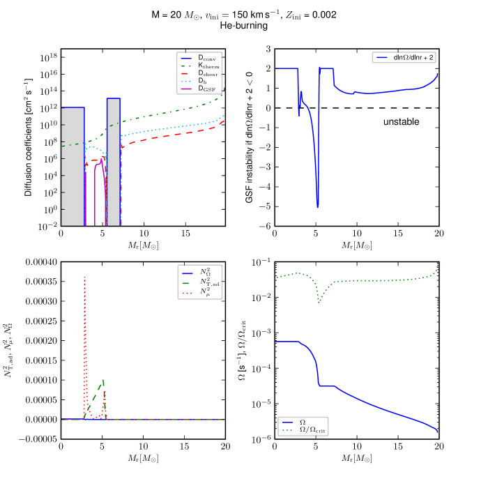
Figure 1: Properties of a 20 M_⊙ model with $Z=0.002$ and an initial rotation velocity of 150 km s^-1 during the He-burning phase, when the central He content is $Y_{\mathrm{c}}=0.543$ and the actual mass 19.795 M_⊙. a) The top left panel illustrates the various diffusion coefficients as functions of the internal mass. The grey areas correspond to convective zones. b) The top right panel shows the profile of the angular velocity $\Omega$–gradient $({\rm d\,ln}\,\Omega/{\rm d\,ln}\,r)+2$. A negative value of this term means instability. c) The left bottom panel shows the various $N^{2}$. d) The right bottom panel shows the profile of $\Omega$ and its ratio to the local critical angular velocity $\Omega_{\mathrm{crit}}.$

We notice several interesting properties.

1. If $N^{2}_{\Omega}<0$, from Eq. (19) we see that the GSF instability is present in a radiative medium whatever the $\mu$– and $T$–gradients are. Thus, these gradients cannot kill the turbulent transport by the GSF instability. However, the size of the effects has to be determined for any given conditions.

2. If the diffusion coefficient $D_{\mathrm{GSF}}$ by the GSF instability is small with respect to $K$ and $D_{\mathrm{h}}$, we have

   $$D_{\mathrm{GSF}}=2\frac{(-N^{2}_{\Omega})}{\left(\frac{N^{2}_{T,\,\mathrm{ad}}}{(K+D_{\mathrm{h}})}+\frac{N^{2}_{\mu}}{D_{\mathrm{h}}}\right)}\;.$$ (21)

   The assumptions $D_{\mathrm{GSF}}\ll K$ and $D_{\mathrm{GSF}}\ll D_{\mathrm{h}}$ are likely, at least at the beginning of the GSF instability when $N^{2}_{\Omega}$ starts becoming negative. Nevertheless, these assumptions need to be verified for the cases of interest in the advanced stages.

3. If $N^{2}_{\mu}\gg N^{2}_{T,\,\mathrm{ad}}$, as is the case in regions surrounding stellar cores, we get from Eq. (19)

   $$\frac{x}{x+D_{\mathrm{h}}}N^{2}_{\mu}+N^{2}_{\Omega}\approx 0\;,$$ (22)

   $$D_{\mathrm{GSF}}\approx 2D_{\mathrm{h}}\frac{(-N^{2}_{\Omega})}{N^{2}_{\Omega}+N^{2}_{\mu}}\;.$$ (23)

   No assumption on the size of $D_{\mathrm{GSF}}$ is made here. Due to the fast central rotation, $D_{\mathrm{h}}$ and the $\Omega$–gradient in regions close to the central core may be large, thus possibly favoring a significant $D_{\mathrm{GSF}}$.

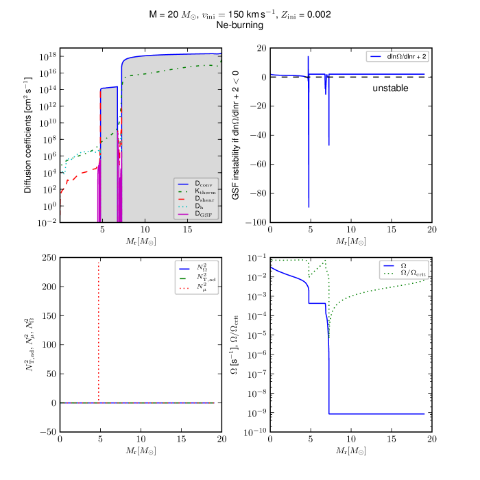
Figure 2: Same as for Fig. 1 during the phase of central Ne–burning. The actual mass is 19.412 M_⊙, the central Ne content is $X(^{20}$Ne)=0.261, the central O–content is $X(^{16}$O)=0.726.

For more general cases, the simple solution of the second order equation (20) has to be used. Most critical of course are the values of $N^{2}_{\Omega}$ and $N^{2}_{\mu}$, which take large values in a narrow region surrounding the central core in the helium and more advanced evolutionary stages.

5 Rotating Stellar Models in the Pre-Supernova Stages

In order to examine quantitatively the importance of the GSF instability, we calculate the evolution all the way from the Main Sequence to the Si burning stage of a 20 M_⊙ star with an initial rotation velocity of 150 km s^-1 with a metallicity Z=0.002 typical of the SMC composition. We make the choice of this composition, because the internal $\Omega$–gradients are steeper at lower $Z$ (Maeder & Meynet (2001)), which would favor the GSF instability. Some data for another 20 M_⊙ model with an initial rotation of 300 km s^-1 are also given. Equation (20) was used to determine the occurence of the GSF instability and the value of $D_{\mathrm{GSF}}$. The above expression (10) for $D_{\mathrm{h}}$ is used. The nuclear network in the advanced phases is the same as in previous models (Hirschi et al. (2004)).

Figure 1 shows in four panels the main parameters during the first part of the phase of central He–burning. We first notice in panel d) the building of a $\Omega$–gradient at the edge of the convective core with a difference of $\Omega$ by about a factor of 20. This makes ${\rm d\,ln}\,\Omega/{\rm d\,ln}\,r+2<0$ in most of the region between the edge of the convective core at 2.9 M_⊙ and the convective H–burning shell at 5.3 M_⊙ as shown in panel b). However $N^{2}_{\Omega}$ remains negligible with respect to $N^{2}_{T}$ and $N^{2}_{\mu}$. In order to understand why, we need to look back at Eq. (15): $N^{2}_{\Omega}=2\overline{\Omega}^{2}(2+\frac{{\rm d\,ln}\,\overline{\Omega}}{{\rm d\,ln}\,r})$. The value of $\Omega^{2}$ in the star is too small to allow a significant value of $N^{2}_{\Omega}$. This means in fact that the centrifugal force in the deep interior is not strong enough to overcome the stabilizing effects of $N^{2}_{T}$ and $N^{2}_{\mu}$ as shown in panel c). The consequence as illustrated in panel a) is that $D_{\mathrm{GSF}}$ remains everywhere smaller than $D_{\mathrm{shear}}$ and is thus not significant. We also notice that $D_{\mathrm{GSF}}$ is always much smaller than $D_{\mathrm{h}}$ and $K$, which permits here the approximation (21) made above.

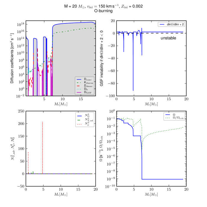
Figure 3: Same as for Fig. 1 during the phase of central O–burning. The actual mass is no longer changing, the central O–content is $X(^{16}$O)=0.692, the central Si–content is $X(^{28}$Si)=0.153.

Figure 2 shows the same plots during the stage of central neon burning. We notice an impressive increase of the central angular velocity and a very small $\Omega$ in the envelope, with a difference by a factor of $10^{8}$ between the two, justifying the examination of the GSF instability. The are two ”$\Omega$–walls”, the big one at 7.2 M_⊙ corresponds to the basis of the H–rich envelope, the other one at 4.8 M_⊙ lies at the basis of the He–burning shell. The values of $({\rm d\,ln}\,\Omega/{\rm d\,ln}\,r)+2$ become much more negative, however over areas of very limited extensions. Again, the value of $N^{2}_{\Omega}$ are negligible, in particular compared to the big peak of $N^{2}_{\mu}$ at 4.8 M_⊙. The result is that $D_{\mathrm{GSF}}$ is always smaller than $D_{\mathrm{shear}}$, even if very locally it can reach about the same value. $D_{\mathrm{GSF}}$ is always at least two or three orders of a magnitude smaller than $D_{\mathrm{h}}$ and $K$, permitting here the simplification (21).

Figure 3 shows the situation in the central O-burning stage slightly less than a year before the central core collapse. Two other small steps in $\Omega$ have appeared near the center, due to the successive ”onion skins” of the pre-supernova model. We notice some new facts. In line with what was already seen for neon burning, the term $({\rm d\,ln}\,\Omega/{\rm d\,ln}\,r)+2$ becomes negative only in extremely narrow regions where the GSF instability is acting with a diffusion coefficient $D_{\mathrm{GSF}}$ larger than in the previous evolutionary stages. Very locally at the upper and/or lower edges of intermediate convective zones, $D_{\mathrm{GSF}}$ may even become larger than $D_{\mathrm{h}}$ and $K$ reaching values above $10^{8}$ cm² s^-1 (there approximation (21) is not valid!). With less than a year left before explosion, the distance over which a significant spread may occur is about $10^{-3}$ R_⊙. This is not entirely negligible in the dense central regions, however this remains of limited importance, as shown by panels b) and d) where we notice that the $\Omega$–walls remain unmodified despite the locally large $D_{\mathrm{GSF}}$.

We may wonder whether higher initial rotation velocities lead to different results. Figure 4 shows the various panels for a similar star in the He–burning phase with an initial rotation velocity of 300 km s^-1. We see that the central rotation velocity is about the same as for the previous case of lower rotation and, in this stage which determines the further evolution, there is no significant difference in the various properties.

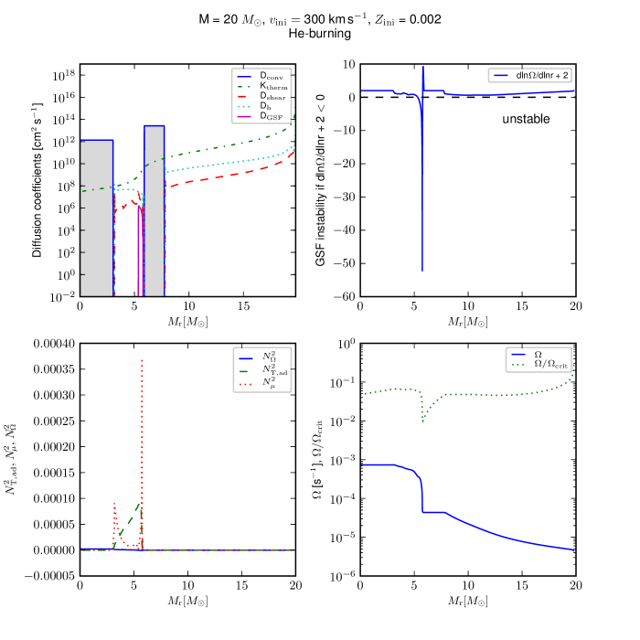
Figure 4: Same as for Fig. 1 for an initial velocity of 300 km s^-1. The star is in the stage of central He–burning with $Y_{\mathrm{c}}$=0.247. The actual mass is 19.681 M_⊙.

6 Conclusions

We have examined the effects of the horizontal turbulence on the GSF instability. This instability is present as soon as $N^{2}_{\Omega}$ is smaller than zero, whatever the effects of the stabilizing $\mu$–gradients.

On the whole, the numerical models of rotating stars show that the diffusion coefficient by the GSF instability grows towards the very latest stages of stellar evolution, however the zones over which it is acting are extremely narrow and there is not enough time left before the supernova explosion for a significant mixing to occur. Thus, even when the inhibiting effect of the $\mu$–gradient is reduced by horizontal turbulence, the GSF instability is unable to smooth the steep $\Omega$–gradients and to significantly transport matter.

We conclude that the amplitude and spatial extension of the GSF instability makes it unable to reduce the angular momentum of the stellar cores in the pre-supernova stages by two orders of magnitude. Therefore, other mechanisms such as magnetic fields (Spruit (2002), Maeder & Meynet (2004), Mathis & Zahn (2005), Zahn et al. (2007)) and gravity waves (Talon & Charbonnel (2005), Mathis et al. (2008)) must be further investigated.

Appendix: some approximations for meridional circulation

The coefficient $D_{\mathrm{GSF}}$ requires, because of the horizontal turbulence, the knowledge of the components $U_{2}$ and $V_{2}$ of the meridional circulation. If the solutions of the 4^th order system of equations governing meridional circulation are not available, some approximations may be considered. We note that the same problem would occur for Eq. (4) by Endal and Sofia (EndalS78 (1978)). As shown by stellar models, the orders of magnitude of $U_{2}$ and $V_{2}$ are the same. The numerical models give in general $V_{2}\sim U_{2}/3$ and $\left|2V_{2}-\alpha U_{2}\right|\sim V_{2}$. Using these orders of magnitude in Eq. (8), we get

$$D_{\mathrm{h}}\,\approx\left(\frac{\beta}{10}\right)^{1/2}\left(r^{2}\,\overline{\Omega}\right)^{1/2}\bigg{(}\frac{r\,U_{2}}{3}\bigg{)}^{\frac{1}{2}}$$ (24)

For $U_{2}$, various expressions can be used taking into account the amount of differential rotation (Maeder (2009)). We can also get an order of magnitude using the approximation for a mixture of perfect gas and radiation with a local angular velocity $\Omega(r)$, ignoring the effects of differential rotation on the circulation velocity and the Gratton-Öpik term which is large only in the outer layers,

$$U_{2}(r)\,=\,\frac{16}{9}\,\frac{\beta}{(32/3)-8\beta-\beta^{2}}\,\frac{L(r)\;r^{2}}{G\,M^{2}_{r}}$$

$$\frac{1}{\left(\nabla_{\mathrm{ad}}-\nabla+\frac{\varphi}{\delta}\nabla_{\mu}\right)}\frac{\Omega^{2}r^{3}}{G\,M_{r}}\,,$$ (25)

where the various quantities have their usual meaning.