Two-particle photoemission from strongly correlated systems: A dynamical-mean field approach

Abstract

We study theoretically the simultaneous, photo-induced two-particle excitations of strongly correlated systems on the basis of the Hubbard model. Under certain conditions specified in this work, the corresponding transition probability is related to the two-particle spectral function which we calculate using three different methods: the dynamical-mean field theory combined with quantum Monte Carlo (DMFT-QMC) technique, the first order perturbation theory and the ladder approximations. The results are analyzed and compared for systems at the verge of the metal-insulator transitions. The dependencies on the electronic correlation strength and on doping are explored. In addition, the account for the orbital degeneracy allows an insight into the influence of interband correlations on the two particle excitations. A suitable experimental realization is discussed.

I Introduction

Correlation among electrons are at the heart of numerous phenomena in condensed matter such as the metal to insulator transition, the emergence of magnetic and orbital ordering and high-temperature superconductivity fulde ; march ; gebhard . Much of today’s understanding of the role of electronic correlation is based on the analysis of the single particle quantities, e.g. the spectral functions, and how these compare with experimental data huf . Among others, a wide spread experimental technique for this purpose is the angle-resolved (single) photoemission spectroscopy, ARPES huf . On the other hand, two-particle quantities are essential for the study of important phenomena such as the optical conductivity mahan . Two particle properties may be classified in general into those associated with the particle-hole, the hole-hole and the particle-particle channels; different techniques are appropriate to access each of these channels. Probably the most studied one of them is the particle-hole channel marini that governs a number of material properties such as the dielectric and the optical response mahan . The particle-particle and the hole-hole channels have been much discussed in connection with the Auger electron spectroscopy (AES) aesbook ; exp1 ; exp2 ; exp3 ; exp4 ; cini ; sawz1 ; gunnar ; marini2 ; drch ; dkud ; nolt90 and the appearance potential spectroscopy (APS) aps ; nolt90 . Early experimental works were focused on simple compounds where the two particle spectra are well modeled by a convolution the single particle spectra. For AES/APS from correlated systems several theoretical works cini ; sawz1 ; gunnar ; marini2 ; drch ; nolt90 ; gonis ; seib1 ; seib2 have been put forward for the evaluation of the two-particle spectral functions, mostly based on the Hubbard model h1 ; h2 ; h3 . Cini and Sawatzky cini ; sawz1 obtained in their pioneering works exact results for a completely filled band within the single-band Hubbard model. A number of subsequent studies for arbitrary fillings were conducted, mainly using the equation of motion method and the ladder approximation. E.g., in the work of Drchal, the equation of motion method was employed to calculate the spectral density of the two-particle valence bands drch based on an approximate single-particle spectral function. Other works dkud ; tdds ; nolt90 utilize the ladder approximation but differ in their treatments of the single particle quantities. In the work of Treglia et al. tdds , the one-particle spectrum is calculated by evaluating the second order perturbation with respect to the Coulomb interaction and with an additional local approximation in order to simplify the calculation. Drchal and Kudrnovsky dkud ; nolt90 employed the self consistent T-Matrix approximation which is valid at a low electron-occupancy. Seibold et al. seib1 proposed a new approach based on the time-dependent Gutzwiller approximation (TDGA) seib2 to calculate the electron-pairing; they compared also their results with those of the bare ladder approximation (BLA).

Figure 1: A schematics of the one-photon, two-electron ($\gamma$,2e) experiment. Upon the absorbtion of a VUV photon with an energy $\omega_{\gamma}$ two electrons are excited into the vacuum and simultaneously detected at the energies $\epsilon_{1},\epsilon_{2}$ and the momenta k₁, k₂.

These works are mostly discussed in connection with AES and/or APS. Recently, an experimental two-particle technique has been developed in which two (indistinguishable) valence-band electrons are emitted and detected with well defined momenta $\mathbf{k}_{1}$ and $\mathbf{k}_{2}$ and specified energies $\epsilon_{1}$ and $\epsilon_{2}$ upon the absorption of one single (vacuum ultra violet, VUV) photon g2e-1 ; g2e0 ; g2e1 ; g2e2 (the method is abbreviated by $(\gamma,2e)$, i.e. one VUV photon in, two electrons out), as schematically shown in Fig.1. Excitations by a single electron or positron have also been realized and a variety of materials ranging from wide band gap insulators to metals and ferromagnets e2e have been investigated. The ($\gamma,2e$) technique is the extension of ARPES to two-particles; from a conceptional point of view one may then expect to access with ($\gamma,2e$) the two-particle spectral properties of the valence band, as indeed shown below explicitly. A distinctive feature of ($\gamma,2e$) is its vital dependence on electronic correlation jber98 , i.e. the two electrons cannot be emitted with one single photon in absence of electronic correlation. The reason for this is the single particle nature of the light-matter interaction in the regime where the experiments are performed. Theoretical studies concentrated hitherto on weakly correlated systems such as simple metals njjp1 ; njjp2 ; njjp3 ; njjp4 ; fb . Consequently the two-particle initial state was modeled by a convolution of two single-particle states with the appropriate energies. The latter were obtained from conventional band-structure calculations based on the density functional theory within the local density approximation. Correlation effects were incorporated in the construction of the interacting two-particle states of the emitted photoelectrons in the presence of the crystal potential. An exception to this approach is the study of ($\gamma,2e$) from conventional superconductor where the BCS theory was employed for the initial state njjp5 . While the theory reproduced fairly well the observed experimental trends, the previous theoretical formulation will certainly breaks down when dealing with strongly correlated materials such transition metal oxides or rare earth compounds with partially filled bands. In particular, features akin to the metal-insulator transitions are not captured with previous studies. Experiments for such materials are currently in preparations. Hence, it is timely to inspect the potential of ($\gamma,2e$) for the study of strongly correlated systems.

In the present work, we will present a general theory for the two-particle photocurrent and inspect the conditions under which the experiment can access information pertinent to the particle-particle spectral function in the presence of strong electron correlations. In particular, we will inspect the particle-particle excitation in Mott systems at the verge of the metallic-insulating transition. For the description of the properties we employ the Hubbard model h1 ; h2 ; h3 and a non-perturbative technique, namely the dynamical mean field theory metvol89 ; revmod96 (DMFT) in combination with quantum Monte Carlo technique (QMC) hirsch . For the calculations of the two particle Green function we will adopt three different ways: The first one is by calculating the single and the two particle spectral functions in the loop of DMFT-QMC self consistently. This ensures the fulfillment of the sum rules. In the second and the third approaches we basically follow the methods mentioned above for the treatment of AES and APS, i.e. we consider the self convolution (first-order perturbation) and the ladder approximation (LA). We use however the single particle spectral function as obtained from DMFT.

The paper is structured as follows: In section II we present a general expression for the two-particle photocurrent and expose its relation to the two-particle Green function. In section III the problem is formulated within the two-band Hubbard model and a discussion is presented on how to disentangle matrix elements information from the ground state two-particle spectral density. In section IV and V we present and analyze the results for the single and two-band Hubbard model and compare the results obtained at various level of approximations. Section VI concludes this work.

II Correlated two-particle photoemission

The ($\gamma,2e$) set up is schematically shown in Fig.1. These experiments are conducted in the regime where the radiation field is well described classically and the time-dependent perturbation theory in the light-matter interaction and the dipole approximations are well justified (low photon density and low photon frequency $\approx 50$ eV). An essential point for our study is that the operator $D_{N}$ for the photon-charge coupling is a sum of single particle operators, i.e. $D_{N}\propto\sum_{i=1}^{N}\mathbf{A}(\mathbf{r}_{i}).\hat{\mathbf{p}}_{i}$ (in first quantization) where $\mathbf{A}$ is the vector potential and $\hat{\mathbf{p}}_{i}$ is the momentum operator of particle $i$. This implies that $D_{N}$ cannot induce direct many-particle processes in the absence of inter-particle correlations that help share among the particles the energy transferred by the photon to one particle which then results in multiparticle excitations. A mathematical elaboration on this point is given in jber98 and also confirmed below. To switch to second quantization we write $\Delta=\sum_{mm^{\prime}}\left<E_{m^{\prime}}(N_{v}-2)\right|\mathbf{A}.(\hat{\mathbf{p}_{1}}+\hat{\mathbf{p}_{2}})\left|E_{m}(N_{v}-2)\right>P_{2}$. The two-particle photocurrent ($J$), summed over the non-resolved initial and final states $n$ and $m$ is determined according to the formula njjp1 ; njjp2

$$J = \frac{\alpha_{0}}{Z}\sum_{N_{v}}\sum_{mn}e^{-\beta E_{n}(N_{v})}\left|\left\langle E_{m}(N_{v}-2)|\Delta|E_{n}(N_{v})\right\rangle\right|^{2}\delta\left(E-[E_{m}(N_{v}-2)-E_{n}(N_{v})]\right)$$ (1)

$$= \frac{\alpha_{0}}{Z}\sum_{N_{v}}\sum_{mn,m^{\prime}m^{\prime\prime}}e^{-\beta E_{n}(N_{v})}M^{\dagger}_{mm^{\prime}}M_{mm^{\prime\prime}}\langle E_{n}(N_{v})|P_{2}^{\dagger}|E_{m^{\prime}}(N_{v}-2)\rangle\langle E_{m^{\prime\prime}}(N_{v}-2)|P_{2}|E_{n}(N_{v})\rangle$$

$$\hskip 56.9055pt\delta(E-[E_{m}(N_{v}-2)-E_{n}(N_{v})]).$$

Here we introduced the short-hand notation $M_{kl}$ for the matrix elements. The photon energy is denoted by $E=\hbar\omega_{\gamma}$, and $\beta$ is the inverse temperature. Furthermore, $\alpha_{0}=4\pi^{2}\alpha/\omega_{\gamma}$, and $\alpha$ is the fine structure constant. $P_{2}=c_{\alpha}c_{\beta}$ stands for the (hole-hole) two-particle operator acting on the state with $N_{v}$ particles with the energy $E_{n}(N_{v})$. $Z$ is the partition function. Under certain conditions specified below (the sudden approximation and for high photoelectron energies), the variation of the matrix elements, when we vary $\omega_{\gamma}$ as to scan the electronic states of the sample, is smooth in comparison to the change of the matrix elements of $P_{2}$. Furthermore, the diagonal elements of $M_{kl}$ are dominant (see below for a justification), i.e. $M_{kl}\approx M$. In this situation Eq.(1) simplifies to ($\rho$ is the density operator).

$$J=\frac{\alpha_{0}}{Z}\sum_{N_{v}}\sum_{mn}e^{-\beta E_{n}(N_{v})}|M_{mm}|^{2}\langle E_{n}(N_{v})|P_{2}^{\dagger}|E_{m}(N_{v}-2)\rangle\langle E_{m}(N_{v}-2)|P_{2}|E_{n}(N_{v})\rangle$$ (2)

$$\hskip 85.35826pt\delta(E-[E_{m}(N_{v}-2)-E_{n}(N_{v})])$$

$$J=\frac{\alpha_{0}M^{2}}{2\pi Z}\sum_{N_{v}n}\int dte^{-\beta E_{n}(N_{v})}\langle E_{n}(N_{v})|e^{iHt}P_{2}^{\dagger}e^{-iHt}\;P_{2}(t=0)|E_{n}(N_{v})\rangle e^{iEt}$$

$$J=\frac{\alpha_{0}M^{2}}{2\pi Z}\int dt\;\mbox{ tr}\left(\rho P_{2}^{\dagger}(t)P_{2}(t=0)\right)\,e^{iEt}$$

$$J=\frac{\alpha_{0}M^{2}}{2\pi}\int dt\ll P_{2}^{\dagger}(t)P_{2}(t=0)\gg\,e^{iEt}.$$

On the other hand, from the spectral decomposition of the two-particle Greens function fetka one infers for the two-particle spectral density $P(\omega)$ the relation

$$P(\omega)=\frac{\alpha_{0}}{Z}\sum_{N_{v}}\sum_{mn}e^{-\beta E_{n}(N_{v})}|\langle E_{m}(N_{v}-2)|P_{2}|E_{n}(N_{v})\rangle|^{2}(1-e^{-\beta\nu})\delta(\omega-E_{m}-E_{n}).$$ (3)

Comparing this equation with Eq.(2) we conclude that under the assumption $M_{kl}\approx M$ the photon-frequency dependence of the two-particle photocurrent is proportional to the two-particle spectral density, i.e.

$$J(\omega)\propto\frac{e^{\beta\omega}}{e^{\beta\omega}-1}P(\omega)$$ (4)

We recall that the two particle spectral function obeys the sum rule

$$\int P(\omega)d\omega=\left<n_{\uparrow}n_{\downarrow}\right>.$$ (5)

A useful auxiliary quantity is partial double occupancy (up to a frequency $\Omega$)

$$K_{p}(\Omega)=\int^{\Omega}d\omega P(\omega).$$ (6)

III Theoretical model

The aim here is to explore the potential of the two-particle photoemission for the study of the two-particle correlations in matter. To do so we start from the generic model that accounts for electronic correlation effects, namely from the doubly degenerate Hubbard Hamiltonian. In standard notation we write h1 ; h2 ; h3

$$H=\sum_{ij\alpha\sigma}t_{\alpha}c_{i\alpha\sigma}^{\dagger}c_{j\alpha\sigma}+U\sum_{i\alpha}n_{i\alpha\uparrow}n_{i\alpha\downarrow}+U^{\prime}\sum_{i\sigma\sigma^{\prime}}n_{i1\sigma}n_{i2\sigma^{\prime}},$$ (7)

where $t_{\alpha}$ describes hopping between nearest neighbor sites $i,j$ for the orbitals $\alpha$$\in$(1,2), $U,U^{\prime}$ stand for the intra- and inter-orbital Coulomb repulsion, respectively. The above Hamiltonian does not account for the exchange interaction, pairing and spin flip processes. The Hubbard model even for a single band provides an insight into a number of phenomena driven by electronic correlations such as the metal-insulator transition which cannot be described usually within a static mean field theory or within an effective single particle picture such as the Kohn-Sham method within the density functional theory. Within the Hubbard model and for the case of infinite connectivity $d\rightarrow\infty$ the self energy turns local metvol89 ; hartmann . This fact has lead to the development of a new powerful computational scheme for the treatment of electronic correlation, namely the dynamical mean field theory (DMFT). For the practical implementation of DMFT it is essential to map the many-body problem onto a single impurity Hamiltonian with an additional self consistency relations geoli92 . Some of the possible applications of DMFT have been discussed in Ref.[revmod96, ], e.g. the long standing problem of the metal insulator transition in the paramagnetic phase is described in a unified manner. From a numerical point of view, solving the impurity Hamiltonian is a challenging task in the self consistency of DMFT. For this purpose, quantum monte carlo (QMC) methods are shown to be an effective approach which we will follow in the present work with the aim to calculate the single and the two particle Green’s functions. We note here that since QMC provides only the data for imaginary times or equivalently at certain Matsubara frequencies, we need to perform analytical continuation to obtain the zero temperatures dynamical quantities. This we do by means of the maximum entropy method that we implemented using the Bryan method. A detailed discussions on this topic can be found in Ref.[Jarrguber, ].

III.1 The matrix elements

Now we have to discuss the validity range of the approximation (3) that enabled us to assume for the matrix elements $M_{kl}\approx M$. We consider the experiments in the configuration shown in Fig.1. The photoelectron momenta $\mathbf{k}_{1}$ and $\mathbf{k}_{2}$ are chosen to be large such that the escape time is shorter than the lifetime of the hole states. For the description of the photoemission dynamics we concentrate therefore on the degrees of freedom of the photo-emitted electrons (which amounts to the sudden approximation). The energy conservation laws reads then (cf. Fig.1)

$$\hbar\omega_{\gamma}-\omega=\varepsilon_{1}+\varepsilon_{2}$$ (8)

where $\omega$ is the initial (correlated) two-particle energy. The single particle energies $\varepsilon_{j}$ are measured with respect to the edge of the valence band (or with respect to the Fermi level $\mu$ in the metallic case). The matrix elements, e.g. $M_{mm^{\prime}}$, reduce in the sudden approximation to two particle transition matrix elements $M_{if}$. The high energy final state (with energies $\varepsilon_{1},\varepsilon_{2}$) we write as a direct product of two Bloch states ($\psi_{\mathbf{k}}$) characterized by the wave vectors $\mathbf{k}_{1}$ and $\mathbf{k}_{2}$, i.e.

$$\Psi_{\mathbf{k}_{1},\mathbf{k}_{2}}(\mathbf{r}_{1},\mathbf{r}_{2})=\psi_{\mathbf{k}_{1}}(\mathbf{r}_{1})\psi_{\mathbf{k}_{2}}(\mathbf{r}_{2}).$$ (9)

III.1.1 Intersite ground state correlation

Correlation effects enters in the initial two particle states. In absence of spin-dependent scattering (as is the case here) it is advantageous to couple the spins of the two initial states to singlet (zero total spin) and triplet (total spin one) states prl99 . In the paramagnetic phase and if the two electrons are not localized on the same sites (they are mainly around $\mathbf{R}_{i}$ and $\mathbf{R}_{j}$ with $i\neq j$) the initial state is a statistical mixture of singlet and triplet states. The radial part we write then as note1

$$\Psi_{\omega}(\mathbf{r}_{1},\mathbf{r}_{2}) = \left[\varphi_{1}(\mathbf{r}_{1}-\mathbf{R}_{i})\varphi_{2}(\mathbf{r}_{2}-\mathbf{R}_{j})\pm\varphi_{1}(\mathbf{r}_{2}-\mathbf{R}_{i})\varphi_{2}(\mathbf{r}_{1}-\mathbf{R}_{j})\right]\chi(|\mathbf{r}_{2}-\mathbf{r}_{1}+\mathbf{R}_{i}-\mathbf{R}_{j}|)$$ (10)

$$= \Psi_{\omega}^{(0)}\chi(|\mathbf{r}_{2}-\mathbf{r}_{1}+\mathbf{R}_{i}-\mathbf{R}_{j}|.$$

The ”plus” (”minus” sign) stands for the singlet (triplet) channel. We note that since the transition operator $D_{2}$ is symmetric with respect to exchange of particles, there is no need to anti-symmetrize the final state (9). In Eq.(10) the function $\varphi_{1}(\mathbf{r}_{1}-\mathbf{R}_{i})$ and $\varphi_{1}(\mathbf{r}_{2}-\mathbf{R}_{j})$ are single particle Wannier orbitals localized at the sites $\mathbf{R}_{i}$ and $\mathbf{R}_{j}$, respectively. $N_{i}$ is the number of sites and $\chi(|\mathbf{r}_{2}-\mathbf{r}_{1}+\mathbf{R}_{i}-\mathbf{R}_{j}|)$ is a (dynamical) correlation factor which we assumed to be dependent on the relative distance between the electrons. The part $\Psi_{\omega}^{(0)}$ contains correlation effects due to exchange only. Due to the localization of the Wannier states around the ionic sites we expect $\chi(|\mathbf{r}_{2}-\mathbf{r}_{1}+\mathbf{R}_{i}-\mathbf{R}_{j}|)$ to decay with increasing $r_{1/2}$ (for $i\neq j$). Since we are dealing with a lattice periodic problem we can express the Wannier functions as the Fourier transform of the Bloch states, i.e. $\varphi(\mathbf{r}-\mathbf{R}_{i})=\frac{1}{N_{i}}\sum_{\mathbf{q}}^{1.BZ}\psi_{\mathbf{q}}(\mathbf{r})e^{-i{\mathbf{q}}\cdot\mathbf{R}_{i}}$ ($1.BZ$ stands for the first Brillouin zone). With this relation and exploiting the orthogonality of the Bloch states we obtain upon straightforward calculation the following expression for the matrix element

$$M_{if} = \langle\Psi_{f}|\mathbf{A}\cdot(\hat{\mathbf{p}}_{1}+\hat{\mathbf{p}}_{2})|\Psi_{i}\rangle$$

$$\approx \frac{1}{N_{i}}\left\{\sum_{\mathbf{q}_{1}\mathbf{q}_{2}}^{1.BZ}\exp(-i{\mathbf{q}_{1}}\cdot\mathbf{R}_{i}-i{\mathbf{q}_{2}}\cdot\mathbf{R}_{j})M^{(1)}_{\mathbf{q}_{1},\mathbf{k}_{1}}\,\delta_{\mathbf{q}_{2},\mathbf{k}_{2}}\pm 1\leftrightarrow 2\right\}\chi(|\mathbf{R}_{i}-\mathbf{R}_{j}|)$$

$$+\int d^{3}r_{1}d^{3}r_{2}\;\Psi_{\mathbf{k}_{1},\mathbf{k}_{2}}^{*}(\mathbf{r}_{1},\mathbf{r}_{2})\Psi_{\omega}^{(0)}\>\mathbf{A}\cdot(\hat{\mathbf{p}}_{1}+\hat{\mathbf{p}}_{2})\chi(|\mathbf{r}_{2}-\mathbf{r}_{1}+\mathbf{R}_{i}-\mathbf{R}_{j}|).$$

. (11)

In this equation $M^{(1)}_{\mathbf{q}_{1},\mathbf{k}_{1}}$ is the matrix element for the conventional single photoemission from the Bloch state $\psi_{\mathbf{q}_{1}}$, i.e. $M^{(1)}_{\mathbf{q}_{1},\mathbf{k}_{1}}=\langle\psi_{\mathbf{k}_{1}}|\mathbf{A}\cdot\hat{\mathbf{p}}_{1}|\psi_{\mathbf{q}_{1}}\rangle$. In deriving the first term of (11) we assumed $\chi(|\mathbf{r}_{2}-\mathbf{r}_{1}+\mathbf{R}_{i}-\mathbf{R}_{j}|)$ to vary smoothly with $r_{1/2}$, i.e. $\chi(|\mathbf{r}_{2}-\mathbf{r}_{1}+\mathbf{R}_{i}-\mathbf{R}_{j}|)\approx\chi(|\mathbf{R}_{i}-\mathbf{R}_{j}|)$ for $i\neq j$. For 3D periodic structure the first two terms of Eq.(11) vanish (momentum and energy conservation laws cannot be satisfied simultaneously). Hence, the transition matrix element is determined by the third term of (11), more precisely by the gradient of the correlation factor $\chi$. If this gradient is smooth on the scale of the variation of $\Psi_{\mathbf{k}_{1},\mathbf{k}_{2}}$ and/or $\Psi_{\omega}^{(0)}$ then the matrix element vanishes all together since $\Psi_{\mathbf{k}_{1},\mathbf{k}_{2}}$ and $\Psi_{\omega}^{(0)}$ are orthogonal. Explicitly we find in this case

$$M_{if} \approx\frac{1}{N_{i}}\sum_{\mathbf{q}_{1}\mathbf{q}_{2}}^{1.BZ}\left\{\exp(-i{\mathbf{q}_{1}}\cdot\mathbf{R}_{i}-i{\mathbf{q}_{2}}\cdot\mathbf{R}_{j})\delta_{\mathbf{q}_{2},\mathbf{k}_{2}}\delta_{\mathbf{q}_{1},\mathbf{k}_{1}}\pm 1\leftrightarrow 2\right\}$$ (12)

$$\hskip 56.9055pt\left.\frac{}{}\mathbf{A}\cdot(\hat{\mathbf{p}}_{1}+\hat{\mathbf{p}}_{2})\chi(|\mathbf{r}_{2}-\mathbf{r}_{1}+\mathbf{R}_{i}-\mathbf{R}_{j}|)\right|_{\mathbf{r}_{2}=0=\mathbf{r}_{1}}.$$

From this expression we conclude that the matrix elements diminish for decreasing correlation $\chi$, in fact for $i\neq j$ this contribution to the pair emission is expected to be marginal due to screening.

III.1.2 On site ground state correlation

The major contribution to the matrix elements is expected to stem from the onsite emission $\mathbf{R}_{i}=\mathbf{R}_{j}$. Only the singlet state is allowed in the single band Hubbard model. To obtain the two-particle wave function we assume in line of the Hubbard model that the two electrons scatter via a contact potential of strength $U$ when they are on the same site. The wave function reads then

$$\bar{\Psi}_{\omega}(\mathbf{r}_{1},\mathbf{r}_{2}) = \left[\varphi_{1}(\mathbf{r}_{1}-\mathbf{R}_{i})\varphi_{2}(\mathbf{r}_{2}-\mathbf{R}_{i})+\varphi_{1}(\mathbf{r}_{2}-\mathbf{R}_{i})\varphi_{2}(\mathbf{r}_{1}-\mathbf{R}_{i})\right]\bar{\chi}(|\mathbf{r}_{2}-\mathbf{r}_{1}|)$$ (13)

$$= \bar{\Psi}_{\omega}^{(0)}\bar{\chi}(|\mathbf{r}_{2}-\mathbf{r}_{1}|).$$

$\bar{\Psi}_{\omega}^{(0)}$ describes the on-site two electron states that include exchange correlation only. Using only $\bar{\Psi}_{\omega}^{(0)}$ yields zero matrix elements as shown above. To obtain an expression for the correlation factor $\bar{\chi}(|\mathbf{r}_{2}-\mathbf{r}_{1}|)$ (that tends to 1 for $U\to 0$) we switch to relative $\mathbf{R}_{-}$ and center of mass coordinates $\mathbf{R}_{+}$. We find that $\bar{\chi}(|\mathbf{r}_{2}-\mathbf{r}_{1}|)$ is determined by the integral (Lippmann-Schwinger) equation ($\chi_{0}$ is determined by asymptotic conditions) $\bar{\chi}(R_{-})=\chi_{0}+U\int d^{3}\mathbf{R}_{-}^{\prime}g^{r}(\mathbf{R}_{-},\mathbf{R}_{-}^{\prime})\delta^{(3)}(\mathbf{R}_{-}^{\prime})\bar{\chi}(\mathbf{R}_{-}^{\prime})$, where $g^{r}$ is the retarded Green’s function in the relative coordinate. For (13) we find then the explicit solution

$$\bar{\Psi}_{\omega}(\mathbf{r}_{1},\mathbf{r}_{2})=\bar{\Psi}_{\omega}^{(0)}(\mathbf{r}_{1},\mathbf{r}_{2})\left[1+\bar{U}g^{r}(\mathbf{r}_{1}-\mathbf{r}_{2},0)\right],\quad\bar{U}=\frac{U}{1-Ug^{r}(0,0)}.{}\hskip 28.45274pt$$ (14)

The key point inferred from this relation is that the two-particle transition amplitude increases as $U$ increases ($\bar{\Psi}_{\omega}^{(0)}$ does not contribute to the matrix elements) and it vanishes for $U\to 0$. It should be noted here that in general $\bar{U}$ is a dynamical quantity, as evident from its definitions.
To summarize this section we can say for fixed momenta $\mathbf{k}_{1},\mathbf{k}_{2}$ of the photoelectrons and for a given $U$, the frequency dependence of the two-particle emission, $J(\omega)$, is related to the frequency dependence of the spectral function $P(\omega)$. For a given $\omega$, the matrix elements vary with $U$; they contribute a $\bar{U}^{2}$ dependence to $J(\omega)$. The additional $U$ dependence of $J(\omega)$ that stems from the spectral function will be inspected below.

III.2 Two-particle Green’s function

For our purpose we utilize the general expression for the two particle propagator

$$\chi^{(\alpha,\sigma),(\alpha^{\prime},\sigma^{\prime})}_{pp}(\mathbf{q},i\omega_{m})=\int\langle T_{\tau}c_{\mathbf{k},\alpha^{\prime}\sigma^{\prime}}(\tau)c_{\mathbf{q}-\mathbf{k},\alpha,\sigma}(\tau)c^{\dagger}_{\mathbf{q}-\mathbf{p},\alpha,\sigma}(0)c^{\dagger}_{\mathbf{p},\alpha^{\prime}\sigma^{\prime}}(0)\rangle.$$ (15)

$\int$ is a short-hand notation for $-\sum_{\mathbf{k},\sigma}\int_{0}^{\beta}d\tau e^{i\omega_{m}\tau}$ and $\omega_{m}=\frac{2m\pi}{\beta}$ is the Matsubara frequency, $T_{\tau}$ is an ordering operator for $\tau$. The local version of the above two particle Green’s function or the onsite s-wave electron pair which will be directly calculated in the self consistency loop of DMFT-QMC is

$$\chi_{pp}(\tau)=\left<T_{\tau}\Delta^{\dagger}(\tau)\Delta(0)\right>\quad\mbox{where}\quad\Delta=c_{\uparrow}c_{\downarrow}.$$ (16)

The evaluation of the two particle propagator may be performed with the aid of the perturbation expansion using the standard diagrammatic theory by selecting the diagrams appropriate for the physical problem at hand. For the Hubbard model with the short range interaction we utilize the ladder-type diagrams. For the single-band Hubbard model (an extension to the multi-orbital case is straightforward), the two particle propagator reads

$$\chi_{pp}(\mathbf{q},i\omega_{m})=-\frac{1}{\beta}\sum_{\mathbf{k}i\nu_{n}}\mathcal{G}(\mathbf{k},i\nu_{n})\mathcal{G}(\mathbf{q}-\mathbf{k},i\omega_{m}-i\nu_{n})\Gamma(\mathbf{k},\mathbf{q},i\omega_{m}).$$ (17)

We selected the ladder diagrams and summed to all orders. Since in our model the Coulomb interaction is static and independent of the wave vector, the vertex function $\Gamma$ reads

$$\Gamma(\mathbf{k},\mathbf{q},i\omega_{m})=1-\frac{U}{\beta}\sum_{\mathbf{p}i\nu_{n}^{\prime}}\mathcal{G}(\mathbf{p},i\nu_{n}^{\prime})\mathcal{G}(\mathbf{q}-\mathbf{p},i\omega_{m}-i\nu_{n}^{\prime})\Gamma(\mathbf{p},\mathbf{q},i\nu_{n}^{\prime}),$$ (18)

meaning that the right hand side of this relation is independent of $\mathbf{k}$ nolt90 . Thus we obtain

$$\chi_{pp}(\mathbf{q},i\omega_{m})=\frac{\chi(\mathbf{q},i\omega_{m})}{1-U\chi(\mathbf{q},i\omega_{m})}$$ (19)

where

$$\chi(\mathbf{q},i\omega_{m})=-\frac{1}{\beta}\sum_{\mathbf{p},i\nu_{n}}\mathcal{G}(\mathbf{p},i\nu_{n})\mathcal{G}(\mathbf{q}-\mathbf{p},i\omega_{m}-i\nu_{n})$$ (20)

is the two particle Green’s function expressed in terms of the full single particle Green’s function. Performing standard analytical continuation and evaluating the imaginary part of the two particle Green’s function one arrives at the following expression for the two particle spectral function

$$P(\omega)=\rm{Im}[\chi_{\textit{pp}}(\mathbf{q},\omega+i\delta)].$$ (21)

In order to evaluate the above equation, it is sufficient to calculate the imaginary part of the two particle propagator $\chi(\omega)$, and analytically continue it to real frequencies. This yields

$$\chi_{i}(\omega)=\mathscr{C}_{0}\int^{\infty}_{-\infty}d\nu\int^{\infty}_{-\infty}d\epsilon D(\epsilon)\left[A(\epsilon,\nu)A(-\epsilon,\omega-\nu)(1-f(\nu)-f(\omega-\nu)\right],$$ (22)

where $\chi_{i}(\omega)$ stands for the imaginary part of $\chi(i\omega)$, $f(\omega)$ is the Fermi distribution function and $A(\epsilon,\omega)=-\frac{1}{\pi}$Im$\left[\frac{1}{\omega-\epsilon-\Sigma(\omega)}\right]$ is the full interacting single particle spectral function. $D(\epsilon)$ is the free density of states and $\mathscr{C}_{0}$ is a constant. The real part of the two particle vertex is obtained via the Kramers-Kronig relation, which follows from the causality condition. For the case of the degenerate Hubbard model, it is straightforward to extend the above formulation where now each Green’s function contains the composite orbital spin index, $\alpha=(\alpha,\sigma)$

$$\chi^{\alpha,\alpha^{\prime}}_{pp}(\mathbf{q},i\omega_{m})=\frac{\chi^{\alpha,\alpha^{\prime}}(\mathbf{q},i\omega_{m})}{1-U\chi^{\alpha,\alpha^{\prime}}(\mathbf{q},i\omega_{m})}.$$ (23)

The two particle propagator $\chi^{\alpha,\alpha^{\prime}}(\mathbf{q},i\omega_{m})$ reads in this case

$$\chi^{\alpha,\alpha^{\prime}}(\mathbf{q},i\omega_{m})=-\frac{1}{\beta}\sum_{\mathbf{p},i\nu_{n}}\mathcal{G}^{\alpha}(\mathbf{p},i\nu_{n})\mathcal{G}^{\alpha^{\prime}}(\mathbf{q}-\mathbf{p},i\omega_{m}-i\nu_{n}).$$ (24)

IV Single Band Hubbard Model

An essential ingredient for the calculation of the two particle Green’s function (22), is the single particle spectral function. The results of the spectral function obtained from DMFT-QMC method for the single band Hubbard model at half filling and away from filling are presented in Fig.2. In the QMC calculation, the Hirsch-Fye hirsch algorithm is employed with the following parameters: The energy scale is set by the bandwidth $W=1$. For the temperature we choose $T/W=0.05$, the increment of time slices is $\Delta\tau<=$0.5. DMFT-QMC calculations are performed for the paramagnetic phase and using the Bethe lattice for the free state density in the self consistency loop.

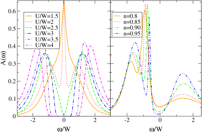
Figure 2: The results of the DMFT-QMC for the frequency dependence of the single-particle spectral function $A(\omega)$ for the single-band Hubbard model at half filling for various interaction strengths $U$ (left panel) and for various electron occupancy at $U/W=3$ (right panel); for all cases we choose $W=1$.

At half filling (the left panel of Fig.2) the quasi-particle peak at the Fermi energy is the dominant feature in the single particle spectra in the weak coupling interaction signifying a metallic behavior; the carriers are itinerant and a Fermi liquid picture is appropriate. With an increasing strength of electronic correlations, localization sets in accompanied by a gradual disappearance of the quasi-particle weight and the formation of a pseudogap. Electron transfer between the two bands may occur, albeit its probability is smaller than that in the previous case. As the coupling strength further increases, the gap fully develops indicating an insulating state.

The role of the double occupancy we inspect by studying the quantity $\left<n_{\uparrow}n_{\downarrow}\right>$ calculated in the DMFT-QMC loop. Evolving from the weakly interacting (metallic) case to the strongly interaction (insulating) phase the double occupancy is reduced revmod96 , for more energy is required to overcome the stronger repulsion whenever forming the double occupation. The influence of dopant concentration on the MIT is demonstrated by doping the insulating phase as depicted in the right panel of Fig.2. Contrasting with the results at half filling with an interaction strength $U/W=3$, the spectral function in this case shows a resonance peak at low energies testifying that the system attains again a metallic character. This is because the doping enhances the number of holes which in turns increases the itineracy such that the electron can hop from one site to the other.

Figure 3: Two particle spectral function as function of the correlated, two-particle initial energy $\omega$ for various interaction strengths. Calculations are performed within the self consistency scheme of DMFT-QMC method. The large scale figure is shown in inset (b). Inset (a) shows the integrated spectra using Eq.(6). Note however, that the energy is measured with respect to the uncorrelated two-particle Fermi energy $2\mu$.

Having commented on the generic single particle properties of the single band Hubbard model for Mott systems, we turn now to the discussion of the particle-particle spectral function. For small $U/W$ one obtains an intense peak that lies close to $\omega/W=0$. The origin of such features can be inferred from the structure of the single particle spectral function: $P$ in this case is well modeled by a convolution of two single-particle spectral functions. A small increase of $U/W$ leads to a reduction of the spectral weight which shifts the peak to higher energeis (far from $\omega/W=0$). As the interaction strength further increases, the spectral weight decreases significantly signaling a reduction of double occupation. This argument is supported by the results of the integrated spectra depicted in the inset of Fig.3. In addition to the reduction of the spectral weight, one also observes the formation of a gap in the low energy regime (near to the zero frequency) for strong interaction. This two particle gap resembles the one that appears in the single particle spectra (cf. Fig.2) which is the usual indicator for an insulating state. We argue here that this is also a signal for the system in the insulating state from the point of view of particle-particle excitations.

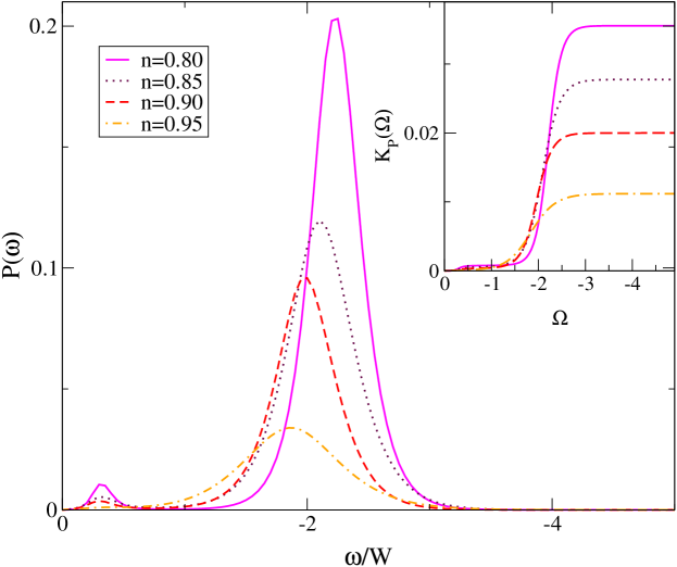
Figure 4: The same as Fig.3 with the same notation, however we inspect here the two particle spectral function away from half filling for $U/W=3$ and for various electron occupancies. Inset shows the integrated spectra according to equation (6).

As already pointed out above, the reappearance of the low energy resonance as a function of the doping is a signal for the metallic character and the associated behavior of the single particle spectral function. The same pattern is also observed in the two particle spectral function where the strongest peak occurs in the lowest electron occupancy and decreases as the Mott insulating phase is approached. Thus the two particle spectra also highlight the contribution of holes to the double occupancy probability, and it is clearly supported by the results for the integrated spectra (see inset of Fig.4).

IV.1 Relation to the ($\gamma,2e$) experiments

To connect the results of Fig.3 to the $(\gamma,2e)$ signal it is decisive to recall the statements of equations (8,14): The correlated two-particle initial energy that appears in Eq.(8) and which is scanned in Fig.3, is in the uncorrelated case merely the sum of two single particle energies $\omega_{i}$ ($\omega_{uncor}=\omega_{1}+\omega_{2}$), i.e. in the metallic uncorrelated case we expect some spectral weight around $\omega=0$ in Fig.3. For a finite $U$, i.e. for a correlated system one requires more energy to compensate for the repulsion of the Coulomb interaction. This is the reason for the shift of the two-particle peak in Fig.3 with increasing $U$. The same can be observed in the single particle spectral function where the distance between the two Hubbard band is approximately on the order of $U/W$. The tendency of larger spectral density with decreasing $U$ is not reflected in the $(\gamma,2e)$ signal $J$. In fact, the opposite will occur. The reason for this is that according to eqs. (14, 2) $J$ is proportional to the product of the matrix elements and the spectral function. On the other hand the matrix elements decrease with $U$ (cf. eqs.(11,14)), and in fact vanishes for $U\to 0$ counteracting against the trend with $U$ of the spectral function $P$ (cf. Fig.3). We stress however, that the results shown in Fig.3 are still relevant to the $(\gamma,2e)$ measurements in that, for a given $U$, the matrix elements are hardly dependent on $\omega$.

IV.2 Comparison between different approaches to the two-particle spectral functions

To inspect the role of the ladder diagram summation (i.e. Eq.(19) with results in Fig.5 (b)), we compare with the results (shown in Fig.5 (a)) of the first-order approximation using (22) (i.e. with the convolution of the single particle spectra). The results of the first order approximation show a smooth, broad Gaussian-like feature in the spectra for all interaction strengths. This is due to the self-convolution that tends to wash out the character of the original function. The presence of a gap in the two-particle spectra highlights the difference between the weak and the strong coupling interactions in agreement with the previous result of DMFT-QMC and with the same energetic origin as discussed above. That this correct energetic shift is reproduced by this simple scheme is the result of using an accurate single particle spectral function. Another point is the evolution of the two particle spectra from the weak through the strong coupling limit and the associated behaviour of the spectral weight. In the scheme used in Fig.5, the weight seems to be comparable for all values of the interaction strengths except for $U/W=2$ which originates from the low shoulder in the spectra of Fig.2. The reduction of the spectral weight is related to the probability of the double occupancy. It is then conceivable to infer that this scheme violates the sum rule for the two particle spectral function (which is dictated by the double occupancy, see Eq.(5). This is endorsed by the results for the integrated spectra shown in the inset of Fig.5 (a). The shift to higher frequencies is due to the presence of the gap. No clear suppression is observed as in Fig.3 and Fig.4.

Figure 5: The frequency dependence of the two-particle spectral function at half filling, calculated with the first-order perturbation approximation (a) and with the full ladder approximation (b). Various curves correspond to different interaction strengths. Inset shows the integrated spectra. The single particle quantities are obtained from DMFT. Same notation and units as Fig.3.

Having obtained the imaginary part of the first order approximation we inspect the influence of the ladder diagram summation on the two particle spectra. The results are presented in Fig.5 (b). In contrast with previous results obtained in the first order approximation, the spectra delivered by DMFT-LA are non-uniform with smooth broad feature and a satellite peak. For the weak interaction strength, the two particle spectra hardly depends on the Coulomb interaction strength. As before no clear reduction of the spectral weight is observed. Interesting features in the DMFT-LA scheme emerge at higher interaction strengths, which from the point of view of the single particle spectra, is already the regime of the insulating phase. Instead of suppressing the spectral weight, the increases of the coupling interaction strength results in a narrow satellite peak. The integrated spectra depicted in the inset of Fig. 5 (b) shed some light on this result. The integrated spectra within the ladder approximation exhibit a suppression of the weight for higher frequencies in contrast to results of the first-order approximation. We remark that in the ladder approximation the suppression of the integrated spectra is not related to a diminishing of the weight of the two particle spectral function but is associated with the width of the spectra that become narrow as the interaction increases. All in all we can conclude for these results that the $(\gamma,2e)$ technique is the appropriate tool for testing the validity of approximate schemes for the two-particle Green’s function.

Figure 6: The same as in Fig. (5), however we inspect here the role of varying the electron occupancy $n$ at an interaction strength of $U/W=3$. (a) shows the first-order approximation results whereas in (b) the predictions of the ladder approximation are plotted.

The two-particle spectral function away from half filling is depicted in Fig.6 for various occupancies and for $U/W=3$; calculations are performed within the first-order approximation and within the ladder approximation. No gap formation in the two particle spectra takes place. This is consistent with the behaviour of the single particle spectral function for which the hole doping of the insulating phase stimulates the formation of quasi- particles. In the first-order approximation, one obtains the usual broad Gaussian-type structure that diminishes as a function of the dopant concentration . A somewhat similar situation is also observed for the results of DMFT-LA. In the latter, however, one observes an intense low-energy peak in the case close to half filling. The peak decreases as the doping increases. The results of both these approaches arein contrast to those obtained via DMFT+QMC where the largest spectral weight is obtained for the high doping concentration. Therefore, these results do not reflect the fact that an additional doping leads to an increase in the double occupancy which is clearly supported by the sum rule results plotted in the inset of Fig.6. Here one observes that the spectral function at the maximum value of the doping obtains the smallest spectral weight. A similar finding has been observed in reference seib1 where the bare ladder approximation (BLA) has been utilized. In their result, the decrease of the electron occupancy also increases the peaks in the spectra, which they assume to be a violation of the two particle sum rule. On the other hand, by using the time-dependent Gutzwiller approximation the opposite situation occurs: The two particle spectral weight diminishes as the Mott insulating phase is approached, which is in line with what we obtained above within the DMFT-QMC.

V Two band isotropic Hubbard model

The single band Hubbard model on which we based our above discussion, is useful for systems with only a single band being close to Fermi energy. To inspect the role of the orbital degrees of freedom, which is known to be important for the properties of strongly correlated systems, a multi-orbital model is needed. It is the aim of this section to study the influence of the orbital degeneracy on the single and two particle spectra.

The results for the single particle spectral function within the two band Hubbard model are presented in Fig.7.

Figure 7: The DMFT-QMC results for the frequency dependence of the single-particle spectral function $A(\omega)$ of the two-band, isotropic Hubbard model at half filling. Various curves corresponds to different interaction strengths $U$ in units of the band width $W$ (here $W=1$). The insets show the orbitally resolved spectral functions for the first (upper inset) and the second band (lower inset).

The results are similar to those obtained within the single band Hubbard model (cf. Fig.3). The metallic phase shows an intense quasi-particle peak that diminishes as the coupling interaction becomes stronger. The formation of the gap for a high interaction strength shows the existence of the insulating phase in this degenerate system. An essential point that distinguishes the Mott transition in the single band from the degenerate band case is the value of the critical coupling necessary to obtain a dip in the spectral function. This behavior is well documented in the works of reference Lu94 employing the Gutzwiller approximation. There, a relation has been established between the critical coupling and the orbital degeneracy. From the orbitally resolved spectral function depicted in the embedded figures, one also learns that each band undergoes the same transition from metal into insulating phase. For anisotropic bandwidth each band undergoes an independent metal insulator transition, a behaviour coined as the orbital selective Mott transition anis02 .

The results of DMFT-QMC calculations for the two particle spectral function are illustrated in Fig.8 that contains the two spectral functions of the total band (a) and the interband (b).

Figure 8: The two-particle spectral function of the degenerate Hubbard model at half filling as a function of the two-particle initial energy $\omega$ measured in units of $W$. The calculations are performed by the DMFT-QMC method including total bands (a) and inter-band (b). The interaction strengths $U$ are varied.

From Fig.8 we see that a small increase of the Coulomb interaction in the weak coupling regime hardly affects the overall spectral weight. Furthermore, increasing the interaction strength leads however to the reduction of the spectra as well as to a shift of the dominant peak to higher energy.

For the case of interband spectra, there is a clear signal of the spectral weight reduction already in the metallic case. As the insulating phase is approached, the two particle spectra show a double-peak structure.

Figure 9: The same as in Fig.(8) for the total bands, however we show in (a) the results of the first order perturbation approximation and in (b) those of the ladder approximation.

The two particle spectra obtained by means of the first order approximation as well as by the ladder approximation are shown in Fig.9 (a) and Fig.9 (b) respectively. The behavior of the two particle spectra in the single band Hubbard model obtained within the same scheme (see Fig.4) (e.g. the gap existence, absence of spectral weight reduction) is also observed in the present case. In the metallic case however there are new features predicted by both approximations namely a double peak structure that disappears in the insulating phase. Other notable features such as the increase of the weight as the coupling strength increases are present in the results of both methods.

Figure 10: The same as in Fig.(9) for the interband Hubbard model at half filling. The figure shows the results of the first order approximation (a) and of the ladder approximation (b).

The integrated spectra of the degenerate model indicate a violation of the sum rule for the two particle spectra by both the first order approximation and the ladder approximation. From the three scheme: QMC-DMFT, first order and ladder approximations, the DMFT-QMC methods provides the more reasonable predictions which practically always obey the sum rule as a constraint on the two particle spectral function. This is because, both the single and the two particle propagators are calculated on an equal footing in the self consistency DMFT. An accurate single particle approach when formulating the two particle propagator nolt90 , does not however guarantee the fulfillment of the sum rules. The use of an accurate approach in the single particle spectra captures however pertinent features such as the gap opening in the insulating state which is also observed in the result of DMFT-QMC.

VI Final remarks and conclusions

We shall now comment on the possible implementation of our proposal. It is a widely accepted wisdom that the single band Hubbard model can be employed to explain the results of single particle or particle-hole properties of vanadium sesquioxide V₂O₃. It is shown revmod96 that the variation of the Coulomb repulsion $U$ is realized by changing the chemical composition or applying hydrostatic pressure. We therefore also argue in this respect that the two-particle properties as we have presented here can be accessed in the similar manner. For the two band Hubbard model, the results can be again implemented to describe the physics of V₂O₃. In this case one can investigate to role of the orbital degrees of freedom. The inclusion of orbital degrees of freedom allows the applications of our model to wider class of systems. As for the experimental geometry, our theory is limited by the fact that the employed self energy is local. Thus, our predictions are best tested by fixing in Fig.1 the momenta of the detected electrons. What should be varied is then the photon energy $\omega_{\gamma}$ . Since the momenta and the energies of the detected electrons are fixed by the experiment, the only quantity which is scanned is the initial correlated two-particle energy $\omega$. A simulation of the experiments for varying momenta and fixed $\omega$ requires an explicitly non-local self-energy which goes beyond the validity of the present model.

To summarize, in this work we explored the potential of two-particle photoemission for the study of two-particle correlations in correlated systems. We identified the conditions under which the two-particle photocurrent is related to the two particle spectral function. Calculations have been performed within the framework of the single and the two band Hubbard model. We performed calculations and compared the results of three different schemes DMFT-QMC, the first-order perturbation and the ladder approximations based on the DMFT single particle spectra. In the single band case, the two particle spectral function evaluated with DMFT-QMC is shown to be dependent on the double occupancy in the system. As for the single particle spectral function, an increase in the electronic correlation strength results in suppression of spectral weight of the two particle spectra and in an opening of a gap near zero two-particle frequency. The first-order perturbation and ladder approximation calculations are qualitatively different from the DMFT-QMC predictions. A finding that can be directly tested by two-particle photoemission spectroscopy. The inclusion of the orbital degeneracy brings about an increase of the critical coupling and additional interband contributions to the spectra; these features should also be distinguishable by two-particle photoemission experiments.

VII Acknowledgments

This work is supported by the international Max-Planck research school for science and technology of nanostructures and by the DFG under contract SFB 762.

References

- (1) P. Fulde, Electron Correlations in Moleculs and Solids (Springer Series in Solid-State Sciences) (Springer, Berlin, 1993).
- (2) N. H. March, Electron Correlation in Molecules and Condensed Phases (Springer, Berlin, 1996).
- (3) F. Gebhard, The Mott Metal-Insulator Transition Models and Methods (Springer, Berlin, 1997); S. Maekawa et al., Physics of Transition Metal Oxides: (Springer Series in Solid-State Sciences vol. 144) The Mott Metal-Insulator Transition Models and Methods (Springer, Berlin, 2004).
- (4) S. Hüfner, Photoelectron Spectroscopy (Springer Verlag, Berlin, 1995); W. Schattke und M. A. Van Hove, Solid-State Photoemission and Related Methods: Theory and Experiment (Wiley-VCH, Weinheim, 2003).
- (5) G. D. Mahan, Many Particle Physics. Series: Physics of Solids and Liquids 3rd ed. (Springer, 2000).
- (6) A. Marini, a many-body approach to the electronic and optical properties of copper and silver in correlation spectroscopy of surfaces, thin films and nanostructure; Eds. J. Berakdar, J. Kirschner (Wiley-VCH, 2004) and further chapters and references therein.
- (7) M. Cini, Solid. State. Commun. 24, 681 (1977).
- (8) C. Verdozzi, M. Cini and A. Marini, J. Elec. Spec. and Related Phenomena 117, 41 (2001).
- (9) V. Drchal, J. Phys. Condens. Matt. 1, 4773 (1989) see also references therein for earlier related works.
- (10) V. Drchal and J. Kudrnovsky, J. Phys. F 14, 2443 (1984).
- (11) J. T. Grant, Surface Analysis by Auger and X-ray Photoelectron Spectroscopy (Chichester: IM Publication, 2003).
- (12) P. Bennett, J. C. Fuggle, F. U. Hillebrecht, A. Lenselink and G. A. Sawatzky, Phys. Rev. B 27, 2194 (1983).
- (13) R. Lof, M. A. van Veenendaal, B. Koopmans, H. T. Jonkman and G. A. Sawatzky, Phys. Rev. Lett. 68, 3924 (1992).
- (14) K. Maiti, D. D. Sarma, T. Mizokawa and A. Fujimori, Phys. Rev. B 57, 1572 (1998).
- (15) R. Gotter, F. Da Pieve, F. Offi, A. Ruocco, A. Verdini, H. Yao, R. Bartynski, and G. Stefani Phys. Rev. B 79, 075108 (2009); A. Liscio, R. Gotter, A. Ruocco, S. Iacobucci, A. G. Danese, R. A. Bartynski, and G. Stefani, J. Elec. Spec. and Related Phenomena 137-140, 505 (2004); R. Gotter, F. Offi, F. Da Pieve, A. Ruocco, G. Stefani, S. Ugenti, M. I. Trioni, and R. A. Bartynski, J. Elec. Spec. and Related Phenomena 161, 128 (2007)
- (16) O. Gunnarsson and K. Schönhammer, Phys. Rev. B 22, 3710 (1980).
- (17) W. Nolting, Z. Phys. B 80, 73 (1990); W. Nolting, G. Geipel, K. Ertl, Z. Phys. B 92, 75-89 (1993).
- (18) G.A. Sawatzky, Phys. Rev. Lett. 39, 504 (1977).
- (19) R.L. Park, J.E. Houston, D.G. Schreiner, Rev. of Sci. Instru, 41, 1810, (1970); R.L. Park and J.E. Houston, Phy. Rev. B 5,10 (1972).
- (20) A. Gonis, J. Elec. Spec. and Related Phenomena 161, 207-215 (2007).
- (21) G. Seibold and J. Lorenzana, Phys. Rev. lett. 94 107006 (2005); G. Seibold, F. Becca, J. Lorenzana, ibid 100, 016405 (2008).
- (22) G. Seibold and J. Lorenzana, Phys. Rev. lett., 86, 2605 (2001).
- (23) J. Hubbard, Proc. R. Soc. London A 276, 238 (1963).
- (24) M. C. Gutzwiller, Phys. Rev. Lett. 10, 159 (1963).
- (25) J. Kanamori, Prog. Theor. Phys. (Kyoto) 30, 275 (1963).
- (26) G. Treglia, M. C. Desjonqueres, F. Ducastelle, and F. Spanjaard, J. Phys. C, 14 4347, (1981).
- (27) R. Herrmann et al., Phys. Rev. Lett. 81, 2148 (1998);
- (28) C. Gazier and J. R. Prescott, Phys. Lett. 32A, 425 (1970); H. W. Biester et al., Phys. Rev. Lett. 59, 1277 (1987 (these experiments did not resolve both the momenta and the energies of the two photoelectrons).
- (29) F.O. Schumann et al. Phys. Rev. Lett. 95, 117601 (2005); Phys. Rev. B 73, 041404(R) (2006); New J. Phys. 9, 372 (2007); Phys. Rev. Lett. 98, 257604 (2007).
- (30) M. Hattass et al. Phys. Rev. B 77, 165432 (2008).
- (31) J. Kirschner et al., Phys. Rev. Lett. 69, 1711 (1992); S. Iacobucci et al., Phys. Rev. B 51, 10252 (1995); O. M. Artamonov et al., Applied Physics A 65, 535 (1997); J. Berakdar et al., Phys. Rev. Lett. 81, 3535 (1998); R. Feder et al., Phys. Rev. B 58, 16418 (1998); S. Samarin et al. Surf. Sci. 579/2-3, 166-174 (2005); Phys. Rev. B 72, 235419 (2005); Phys. Rev. Lett, 85, 1746-1749 (2000); F.O. Schumann et al., Phys. Rev. Lett. 95, 117601 (2005); S. Samarin et al. Phys. Rev. B 76, 125402 (2007); ibid 70 073403 (2004); S. Samarin et al. Phys. Rev. Lett. 97, 096402 (2006); G. van Riessen , et al. J. Phys.: Condensed Matter 20, 442001/1-5 (2008).
- (32) J. Berakdar, Phys. Rev. B 58, 9808 (1998).
- (33) N. Fominykh, J. Henk, J. Berakdar, and P. Bruno, Surf. Sci, 507-510, 229 (2002).
- (34) N. Fominykh, J. Henk, J. Berakdar, and P. Bruno, Phys. Rev. Lett. 89, 086402 (2002).
- (35) N. Fominykh, J. Henk, J. Berakdar, P. Bruno, H. Gollisch, R. Feder, Solid State Communications 113, 665-669 (2000).
- (36) J. Berakdar, H. Gollisch, and R. Feder, Solid State Communications 112, 587-591 (1999).
- (37) N. Fominykh and J. Berakdar, J. Elec. Spec. and Related Phenomena 100, 20 (2007).
- (38) K. A. Kouzakov , J. Berakdar, Phys. Rev. Lett. 91, 257007 (2003); J. Elec. Spec. and Related Phenomena 161, 121-124 (2007).
- (39) W Metzner and D Vollhardt, Phys. Rev. Lett, 62 324 (1989).
- (40) A. Georges, G. Kotliar, M. Rozenberg, and W. Krauth, Rev. Mod. Phys. 68, 13 (1996) and references therein.
- (41) J. E. Hirsch and R. M. Fye, Phys. Rev. Lett. 56, 2521 (1986).
- (42) A Fetter and J.D Walecka. Quantum Theory of Many Particle System. (McGraw-Hill Inc, New-York, 1971).
- (43) E. Müller-Hartmann, Z Phys. B 74, 507 (1989).
- (44) A. Georges and G. Kotliar, Phys. Rev. B 45, 6479 (1992).
- (45) J. Berakdar, Phys. Rev. Lett. 83, 5150-5153 (1999).
- (46) V. I. Anisimov, I. A. Nekrasov, D.E. Kondakov, T. M. Rice, and M. Sigrist, Eur. Phys. J. B 25, 191 (2002).
- (47) M. Jarrell and J.E. Gubernatis. Phys. Rep, 269:133, 1996.
- (48) J.P. Lu, Phys. Rev. B 49, 5687 (1994).
- (49) This form of the wave function is not the most general one. It neglects three-body (and higher) interactions. As discussed in Ref.[jamal_book, ], this doing is well justified for relatively small momentum transfer (on the scale of the Fermi momentum), i.e. distant interactions. An exmaple for the mathematical expressions of the neglected terms is given in jamN .
- (50) J. Berakdar, Concepts of Highly Excited Electronic Systems (Wiley-VCH, Berlin, 2003).
- (51) J. Berakdar, Phys. Rev. A 55, 1994 (1997).