A CCD photometric study of the late type contact binary EK Comae Berenices

Abstract

We present CCD photometric observations of the W UMa type contact binary EK Comae Berenices using the 2 metre telescope of $IUCAA$ Girawali Observatory, India. The star was classified as a W UMa type binary of subtype-W by Samec et al. (1996). The new V band photometric observations of the star reveal that shape of the light curve has changed significantly from the one observed by Samec et al. (1996). A detailed analysis of the light curve obtained from the high-precision CCD photometric observations of the star indicates that EK Comae Berenices is not a W-type but an A-type totally eclipsing W UMa contact binary. The photometric mass ratio is determined to be 0.349 $\pm$ 0.005. A temperature difference of $\Delta T=141\pm 10$ K between the components and an orbital inclination of $i[^{o}]=89.800\pm 0.075$ were obtained for the binary system. Absolute values of masses, radii and luminosities are estimated by means of the standard mass-luminosity relation for zero age main-sequence stars. The star shows O’Connell effect, asymmetries in the light curve shape around the primary and secondary maximum. The observed O’Connell effect is explained by the presence of a hot spot on the primary component.

1 Introduction

The eclipsing binary EK Comae Berenices [hereafter EK Com] was discovered by Kinman et al. (1966). They classified the star as a W UMa type binary. The star was also observed visually by Borovicka (1990) who determined the period of $0.2666864$ days. The first photometric solution of EK Com was obtained by Samec et al. (1996, hereafter SA96) based on the observations of 1994 with the help of the Wilson-Devinney [hereafter WD] code. These authors determined a period of 0.2668726 days and derived other photometric elements from their observed light curves and found the evidence for a period decrease at a rate of $\sim 1.5\times 10^{-10}\rm cycle^{-1}$. From the light curve solutions using the WD code, they classified the star as a W UMa type binary of subtype W with a mass ratio $q=0.304$, a temperature difference of $\Delta T=310$ K between the components and a fill-out factor of 15%. They estimated the temperatures of the components as $T_{1}=5000$ K and $T_{2}=5310$ K respectively, where the subscripts 1 and 2 refer to the more massive (primary) and the less massive (secondary) component respectively. The change in the orbital period of EK Com has been analysed by Li and Zhang (2006) and found the evidence of continuous decrease of orbital period $dP/dt=-5.96~{}\times 10^{-10}$ days cycle${}^{-1}=-0.071$ s yr^-1.

Since there is no photometric measurement of the star available since 1994, we have obtained a complete and well-defined light curve of EK Com through high-precision CCD photometry using the $IUCAA$ Girawali Observatory (IGO) 2-m telescope. The newly obtained light curve is quite different in shape than that obtained by SA96. SA96 classified it as a W UMa binary of subtype-W by pointing out that the light curve showed an interval of constant light in the primary eclipse. However, it is difficult to make out whether a minimum is curved or flat and SA96 modelled the light curve assuming a flat-bottom primary minimum. Using the new observations, we are able to present highly accurate and more precise light curve of EK Com than SA96. Based on the appearance of the eclipses in our data, we conclude that the system is clearly an A-type W UMa binary, i.e, the deeper eclipse is the transit of the more massive star by the less massive one. Our new photometric observations, in fact, clearly suggest that the primary minimum is rounded and the secondary minimum is flat indicating its A-type nature.

In this paper, we report the complete V band light curve analysis of the star EK Com from new photometric observations and employ the WD light curve modelling technique. This technique is used extensively to characterize the observed photometric light curves of eclipsing binary stars with the computed synthetic light curves thus yielding the parameters of components of the binary system. It has been seen from the literature that determination of photometric mass ratio $q$ obtained from the WD light curve modelling is reliable only for a total-eclipse configuration of the binary system as such light curves show characteristic inner contacts with duration of totality setting a strong constraint on the $(q,i)$ pair (Rucinski, 2001). Since EK Com is found to be a total-eclipsing over-contact binary, the various geometrical and physical parameters obtained from the light curve modelling are expected to be reliable. Although we have only two nights of data observed only in the V band, the phase coverage is excellent enough to reveal the accurate shapes of the primary and secondary minima. In Section 2, we present the observations and data reduction procedures. Section 3 deals with the period analysis and determination of ephemeris from new observations. In Section 4, we describe detailed photometric analysis of the star in the V band using the WD code. In Section 5, we describe determination of distance to EK Com. Finally, in Section 6, we summarise the results and main conclusions of our study.

2 Observations and data reduction

All the V band CCD photometric observations of the star were carried out with the 2-m IGO telescope, located about 80 km from Pune, India during two nights on March 30 and April $01$ in 2009. The IUCAA Faint Object Spectrograph Camera (IFOSC) equipped with EEV 2 K $\times$ 2 K thinned, back-illuminated CCD with 13.5 $\mu m$ pixels was used. The CCD used for imaging provides an effective field of view of $10.5^{{}^{\prime}}\times 10.5^{{}^{\prime}}$ on the sky corresponding to a plate scale of 0.3 arcsec pixel^-1. The gain and read out noise of the CCD camera are 1.5 e^-/ADU and 4 e^- respectively. The FWHM of the stellar image varied from 3 to 5 pixels during the observations. We took a total of 296 frames in the V band with the exposure times varied between 10s to 60s for a good photometric accuracy.

The co-ordinates of the variable, comparison star and the check star are listed in Table 1. The comparison and the check stars are close to the variable and they are in the same field of view during the observations. The comparison star used here is the same used as a check star by SA96. The standard $V$-magnitude of the comparison star is 12.06 $\pm$ 0.01 (SA96). In Fig. 1, we show a $\sim 10^{{}^{\prime}}\times 10^{{}^{\prime}}$ image of the field with EK Com at centre taken from ESO Online Digitized Sky Survey.

Several bias frames and twilight flatfield frames were taken with the CCD camera to calibrate the images of the stars using standard techniques. Data reduction was carried out using IRAF and MIDAS softwares. The raw images were processed following the standard procedures to remove the bias, trim the images and divide by the mean sky flatfield. The resulting images are therefore free from the instrumental effects. Instrumental magnitudes were obtained using the DAOPHOT package (Stetson, 1987, 1992). The various tasks, e.g., find, phot, daogrow, daomatch and daomaster were applied in order to obtain the instrumental magnitudes of stars in all the frames. Extinction corrections were ignored as the target star is very close to the comparison star. In Fig. 2, we show the plots of the V band magnitudes of (Variable $-$ Comparison) versus Heliocentric Julian Day (HJD) in the upper and lower panels respectively for observations on March 30 and April 01, 2009 and in Fig. 3, we plot the magnitude differences between the comparison and check star (Comp $-$ Check) versus HJD in the upper and lower panels respectively for observations on the respective days.

The reduced results show that the difference between the magnitude of the check star and that of the comparison star was constant with a probable error of $\pm$0.006 mag in the V band. In Table 2, we list the time of observations in HJD and the differential magnitudes of the star with respect to the comparison star ($\rm\Delta V$).

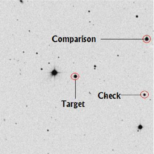
Figure 1: A $\sim 10^{{}^{\prime}}\times 10^{{}^{\prime}}$ image of the field with EK Com at centre taken from ESO Online Digitized Sky Survey. The target star, comparison star and the check star are marked. The range of RA along the horizontal axis is ($\rm 12^{h}~{}51^{m}~{}43^{s}.40,~{}12^{h}~{}50^{m}~{}58^{s}.57$) and that of DEC along the vertical axis is ($27^{\rm o}~{}08^{{}^{\prime}}~{}42^{{}^{\prime\prime}}.20,~{}27^{\rm o}~{}18^{{}^{\prime}}~{}40^{{}^{\prime\prime}}.80$).

Figure 2: Upper and lower panels show the differential magnitudes versus time (in HJD) of EK Com with respect to the comparison star for observations on March 30, 2009 and April 01, 2009 respectively.

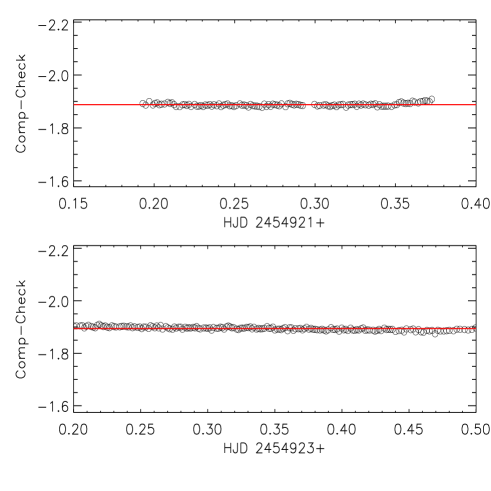
Figure 3: Upper and lower panels show the magnitude differences between the comparison and check star versus time (in HJD) for observations on March 30, 2009 and April 01, 2009 respectively. A solid straight line is drawn at the mean of the differential magnitude data points to show the constancy of variation between the comparison and check star during the course of observations.

Table 1: Coordinates and V band magnitudes of the variable star EK Com, comparison star and check star

Star	RA (J2000)	DEC (J2000)	V mag
EK Com	$12^{\rm h}\,51^{\rm m}\,21^{\rm s}.45$	$27^{\rm o}\,13^{\rm{}^{\prime}}\,47^{\rm{}^{\prime\prime}}.03$	12.021
Comparison	$12^{\rm h}\,51^{\rm m}\,01^{\rm s}.10$	$27^{\rm o}\,16^{\rm{}^{\prime}}19^{\rm{}^{\prime\prime}}.70$	12.060
Check	$12^{\rm h}\,51^{\rm m}\,01^{\rm s}.40$	$27^{\rm o}\,12^{\rm{}^{\prime}}\,43^{\rm{}^{\prime\prime}}.00$	13.998

Table 2: V Band CCD observations of EK Com

HJD		HJD		HJD		HJD		HJD		HJD
(2,454,000 +)	$\rm\Delta V$	(2,454,000 + )	$\rm\Delta V$	(2,454,000 +)	$\rm\Delta V$	(2,454,000 +)	$\rm\Delta V$	(2,454,000 +)	$\rm\Delta V$	(2,454,000 +)	$\rm\Delta V$
921.1929	0.055	921.2671	0.343	921.3440	0.189	923.2508	0.635	923.3288	0.059	923.4080	0.213
921.1948	0.060	921.2684	0.319	921.3453	0.200	923.2523	0.623	923.3302	0.068	923.4095	0.197
921.1970	0.070	921.2698	0.291	921.3475	0.226	923.2538	0.607	923.3316	0.080	923.4110	0.184
921.1993	0.082	921.2711	0.271	921.3494	0.252	923.2559	0.553	923.3330	0.084	923.4125	0.165
921.2006	0.095	921.2724	0.249	921.3507	0.268	923.2574	0.511	923.3344	0.093	923.4144	0.152
921.2019	0.099	921.2738	0.230	921.3521	0.284	923.2588	0.489	923.3364	0.108	923.4159	0.147
921.2032	0.107	921.2751	0.214	921.3535	0.313	923.2605	0.446	923.3378	0.112	923.4174	0.135
921.2046	0.117	921.2764	0.200	921.3549	0.328	923.2620	0.422	923.3393	0.117	923.4189	0.125
921.2064	0.134	921.2777	0.186	921.3563	0.357	923.2634	0.390	923.3407	0.132	923.4204	0.118
921.2086	0.148	921.2791	0.162	921.3577	0.380	923.2648	0.358	923.3422	0.143	923.4232	0.104
921.2098	0.163	921.2817	0.154	921.3591	0.408	923.2663	0.325	923.3442	0.165	923.4247	0.094
921.2111	0.170	921.2830	0.149	921.3605	0.441	923.2688	0.287	923.3457	0.175	923.4262	0.091
921.2124	0.186	921.2843	0.146	921.3619	0.473	923.2702	0.251	923.3471	0.198	923.4277	0.081
921.2137	0.199	921.2856	0.130	921.3641	0.520	923.2716	0.237	923.3486	0.221	923.4292	0.074
921.2159	0.237	921.2870	0.122	921.3655	0.551	923.2737	0.214	923.3500	0.237	923.4316	0.067
921.2176	0.263	921.2883	0.121	921.3669	0.581	923.2751	0.202	923.3518	0.270	923.4331	0.065
921.2190	0.286	921.2896	0.113	921.3683	0.607	923.2765	0.178	923.3533	0.300	923.4346	0.060
921.2203	0.313	921.2910	0.099	921.3697	0.620	923.2784	0.153	923.3547	0.322	923.4361	0.056
921.2216	0.341	921.2923	0.095	921.3711	0.630	923.2798	0.143	923.3562	0.355	923.4376	0.053
921.2230	0.373	921.2996	0.067	921.3725	0.641	923.2811	0.133	923.3576	0.392	923.4399	0.044
921.2252	0.422	921.3015	0.062	923.2001	0.127	923.2831	0.120	923.3595	0.433	923.4424	0.046
921.2265	0.453	921.3028	0.058	923.2021	0.142	923.2845	0.106	923.3610	0.469	923.4446	0.040
921.2278	0.484	921.3053	0.059	923.2050	0.158	923.2858	0.102	923.3624	0.508	923.4463	0.042
921.2292	0.521	921.3067	0.051	923.2065	0.166	923.2871	0.090	923.3638	0.542	923.4481	0.043
921.2305	0.552	921.3080	0.052	923.2080	0.177	923.2890	0.078	923.3653	0.576	923.4513	0.043
921.2319	0.585	921.3093	0.050	923.2095	0.190	923.2903	0.074	923.3676	0.618	923.4531	0.048
921.2332	0.613	921.3106	0.049	923.2110	0.205	923.2917	0.063	923.3691	0.626	923.4550	0.053
921.2345	0.637	921.3120	0.050	923.2131	0.228	923.2930	0.055	923.3706	0.628	923.4571	0.057
921.2358	0.629	921.3133	0.053	923.2146	0.243	923.2943	0.049	923.3721	0.632	923.4590	0.064
921.2372	0.633	921.3146	0.052	923.2161	0.261	923.2969	0.036	923.3736	0.635	923.4608	0.071
921.2390	0.641	921.3160	0.055	923.2176	0.285	923.2987	0.030	923.3755	0.635	923.4633	0.083
921.2403	0.636	921.3173	0.054	923.2191	0.304	923.3001	0.024	923.3770	0.634	923.4653	0.093
921.2416	0.638	921.3193	0.056	923.2206	0.330	923.3014	0.021	923.3785	0.632	923.4672	0.099
921.2430	0.642	921.3206	0.062	923.2221	0.353	923.3028	0.018	923.3800	0.632	923.4695	0.116
921.2443	0.643	921.3219	0.064	923.2237	0.377	923.3042	0.018	923.3815	0.633	923.4714	0.129
921.2456	0.642	921.3232	0.070	923.2252	0.407	923.3066	0.010	923.3837	0.636	923.4734	0.139
921.2470	0.641	921.3246	0.076	923.2267	0.439	923.3080	0.011	923.3852	0.640	923.4759	0.164
921.2483	0.640	921.3259	0.078	923.2285	0.474	923.3094	0.010	923.3867	0.636	923.4780	0.180
921.2496	0.645	921.3272	0.085	923.2300	0.513	923.3108	0.007	923.3882	0.622	923.4801	0.198
921.2509	0.642	921.3286	0.091	923.2315	0.543	923.3122	0.011	923.3897	0.597	923.4832	0.230
921.2533	0.640	921.3299	0.099	923.2344	0.604	923.3140	0.010	923.3919	0.542	923.4856	0.264
921.2546	0.622	921.3312	0.111	923.2359	0.627	923.3153	0.016	923.3934	0.504	923.4880	0.303
921.2560	0.604	921.3334	0.124	923.2374	0.642	923.3166	0.018	923.3949	0.465	923.4913	0.355
921.2573	0.572	921.3347	0.129	923.2394	0.650	923.3180	0.022	923.3964	0.428	923.4941	0.405
921.2586	0.534	921.3360	0.137	923.2409	0.656	923.3193	0.023	923.3979	0.396	923.4969	0.462
921.2599	0.505	921.3374	0.146	923.2424	0.663	923.3215	0.029	923.3998	0.352	923.4997	0.531
921.2613	0.474	921.3387	0.153	923.2439	0.659	923.3229	0.036	923.4014	0.319
921.2626	0.441	921.3400	0.159	923.2454	0.661	923.3243	0.039	923.4029	0.296
921.2639	0.403	921.3414	0.167	923.2478	0.653	923.3257	0.050	923.4044	0.269
921.2653	0.374	921.3427	0.177	923.2493	0.649	923.3271	0.053	923.4065	0.240

3 Period analysis and determination of ephemeris of EK Com

A period analysis was carried out using multiharmonic ANOVA algorithm developed by Schwarzenberg-Czerny (1996, hereafter SC96) to find out the period of EK Com. The method computes periodogram by fitting multiharmonic Fourier series to the time series data. It is very efficient and robust for non-sinusoidal signals. The various statistical properties and the advantages of this method are described in SC96. The following times of minima were determined from the data using the method given by Kwee and van Woerden (1956):

$$\rm Pri.~{}\rm minima=2454923.24382(7)$$

$$\rm Sec.~{}\rm minima=2454921.24434(6),2454923.37792(5)$$

The numbers given in parentheses represent the probable errors. We use the following ephemeris to derive the phased light curve.

$$\rm MinI=\rm HJD\,2454923.24382(7)+0^{d}.26674\times E,$$ (1)

where E is the epoch in days. With 2454923.24382 as the time of the primary eclipse, we plot the phased light curve of the star in Fig. 4 which is defined as an array of phase ($\Phi$) and differential V band magnitude ($\rm\Delta V$). The term phase ($\Phi$) is defined as :

$$\Phi=\frac{\left(t-t_{0}\right)}{P}-Int\left(\frac{t-t_{0}}{P}\right).$$ (2)

The value of $\Phi$ is from 0 to 1, corresponding to a full cycle of the orbital period and $Int$ denotes the integer part of the quantity. The zero point of the phase corresponds to the time of the primary eclipse ($t_{0}$).

Figure 4: Phased light curve of EK Com. The light curve is plotted in the phase range [0, 1.5] for a better view of the two minima. Open circles denote the observational data points.

4 Photometric analysis using the WD code

The photometric analysis of EK Com was done by the WD code as implemented in the software PHOEBE (Prša and Zwitter, 2005). It is a modified package of the widely used WD program for eclipsing binary stars (Wilson and Devinney, 1971; Wilson, 1979, 1990).

The appearance of the eclipses in our data shows that EK Com is likely an A-type rather than a W-type system, implying that the deeper eclipse is the transit of the massive star by the less massive one. From Fig. 4, it is clearly seen that the V-band light curve presents a flatter bottom secondary eclipse covering approximately $0.1$ in phase; this possibly indicates a total-eclipse configuration of the system. The flatter secondary eclipse is obviously shallower than the rounded primary one. It implies that the system is more likely an A-type W UMa binary. It seems that EK Com has evolved from W to A type and resembles AH Cnc which went from W to A type in a time less than a decade (Sandquist and Shetrone, 2003; Zhang et al., 2005).

We define the massive primary component as star 1 and the less massive component as star 2 in the analysis that follows. The effective temperature of the primary component can be calculated from the period-color relation given by Rucinski (2001) who derived the following period-color relation for contact binary systems.

$$(B-V)=0.04\,P^{-2.25},$$ (3)

where $P$ is the period in days. With the above equation, the color of EK Com can be calculated as: $(B-V)$ = 0.782. The interstellar extinction along the direction of EK Com is $E(B-V)=0.010$ following Schlegel et al. (1998). Therefore the intrinsic color index of the star would be $(B-V)_{0}=0.772$. On the other hand, the infrared color index for the star is $(J-K)=0.560$ following Cutri et al. (2003). Both these color indices suggest a spectral type nearly $\rm K{0}V$ for the binary system.

We take the temperature of the star 1 $T_{1}=5150~{}K$ suitable for the spectral type $\rm K0V$ through the calibration of Cox (2000). The gravity-darkening exponents were taken to be $g_{1}=g_{2}=0.32$ according to Lucy (1967) and albedos adopted as $A_{1}=A_{2}=0.5$ following Ruciński (1969). The monochromatic $(x_{1V},x_{2V},y_{1V},y_{2V})$ and bolometric $(x_{1bol},y_{1bol},x_{2bol},y_{2bol})$ limb-darkening coefficients of the components were interpolated for square root law from van Hamme (1993) tables. The adjustable parameters are the mass ratio $q$, orbital inclination angle $i$, the mean temperature of the secondary $T_{2}$, the surface potentials of the components $\Omega_{1}$ and $\Omega_{2}$, and the monochromatic luminosity of the star 1 $L_{1}$ (the planck function was used to compute the luminosity).

To search for a reliable mass ratio $q$, we made test solutions at the outset. The test solutions were computed at a series of assumed mass ratios $q$, with the values from $0.25$ to $0.5$ in steps of 0.1, although SA96 quoted a $q=0.304$ for EK Com. Assuming that it is a detached system, the differential corrections were started from the mode 2 and rapidly ran into mode 3 (contact). After several iterations, a convergent solution was obtained for each assumed value of $q$. From Fig. 5, it can be seen that resulting sum of the squared deviations $\sum\omega_{i}(O-C)^{2}$ of the convergent solutions for each value of $q$ show that the fit is best in the case of $q=0.35$. Starting from the DC solutions at $q=0.35$, we ran the code again and let the mass ratio be adjusted freely along with the other adjustable parameters. The mass ratio converged to a value of $q=0.349$ in the final solution. This value of $q$ indicates that EK Com is a A-subtype W UMa binary. With $q=0.349$, the final solution of the system was obtained. The derived photometric parameters are listed in Table 3. The radii $r$ given in Table 3 are normalised to the semi-major axis of the binary system, i.e., $r=R/a$. The component radii are taken as the geometrical mean of the polar, side and back radii. Fig. 6 shows the theoretical light curve computed with these parameters.

It is very clear that the theoretical light curve does not fit the observational data very well, especially around the quadrature levels. The observed light curves are asymmetric, with the primary maximum brighter than the secondary maximum. This kind of phenomenon of unequal heights at quadrature levels, called O’Connell (1951) effect exists in many binaries. We assumed a hot or a cool spot located on either the primary or secondary component. We found convergent and stable solutions with a hot spot on the primary component. Spot parameters, listed in Table 3 are co-latitude $\phi$, longitude $\theta$, angular diameter $r_{s}$, and the temperature factor $T_{s}/T_{\star}$ ($T_{s}$ is the temperature of the spot, and $T_{\star}$ is the local effective temperature of the surrounding photosphere). The solid line in Fig. 7 shows the fit to the light curve considering a hot spot on the primary component. The corresponding configurations of EK Com with a hot spot on the primary component are plotted in Fig 8.

The fill-out factor or degree of over-contact ($f$) is given by

$$f=\frac{\Omega_{\rm in}-{\Omega}}{\Omega_{\rm in}-\Omega_{\rm out}},$$ (4)

where $\Omega_{\rm in}$ and $\Omega_{\rm out}$ refer to the inner and the outer Lagrangian surface potentials respectively and $\Omega$ represents the dimensionless potential of the surface of the common envelope for the system. The degree of over-contact was determined to be 33.0%.

Figure 5: Sum of the square of the residuals $\Sigma\omega(O-C)^{2}$ as a function of the mass ratio ($q$). The minimum of $\Sigma\omega(O-C)^{2}$ occurs at $q=0.35$.

Table 3: Photometric solutions of the Eclipsing binary EK Com

Parameters	with ‘no spot’	With ‘spot’ on star 1
$q$	0.349 $\pm$ 0.005	0.346 $\pm$ 0.005
$i[^{o}]$	89.800 $\pm$ 0.075	89.808$\pm$ 0.085
$L_{1}/(L_{1}+L_{2})$	0.689 $\pm$ 0.002	0.689 $\pm$ 0.002
$x_{1V}$ = $x_{2V}$	0.526	0.526
$y_{1V}$ = $y_{2V}$	0.256	0.256
$x_{1bol}$ = $x_{2bol}$	0.218	0.218
$y_{1bol}$ = $y_{2bol}$	0.452	0.452
$\Omega_{1}=\Omega_{2}$	2.501 $\pm$ 0.003	2.521 $\pm$ 0.003
$\Omega_{\rm in}$	2.572	2.566
$\Omega_{\rm out}$	2.357	2.352
$T_{1}$	5150 K	5150 K
$T_{2}$	5291 $\pm$ 10 K	5307 $\pm$ 5 K
$A_{1}=A_{2}$	0.500	0.500
$g_{1}=g_{2}$	0.320	0.320
$\sum$	0.054	0.016
$r$(pole):
star 1	0.4568 $\pm$ 0.0006	0.4549 $\pm$ 0.0005
star 2	0.2861 $\pm$ 0.0007	0.2826 $\pm$ 0.0005
$r$(side):
star 1	0.4926 $\pm$ 0.0009	0.4899 $\pm$ 0.0007
star 2	0.3002 $\pm$ 0.0009	0.2960 $\pm$ 0.0007
$r$(back):
star 1	0.5236 $\pm$ 0.0012	0.5199 $\pm$ 0.0009
star 2	0.3446 $\pm$ 0.0016	0.3377 $\pm$ 0.0012
Spot:
$\phi[^{\rm o}]$	$...................$	90.000
$\theta[^{\rm o}]$	$...................$	260.933
$r_{s}[^{\rm o}]$	$....................$	16.000
$T_{s}/T_{\star}$	$....................$	1.097

Figure 6: Solid line shows the synthetic light curve computed with the parameters given in Table 3 with no ‘spot’ considered on the components. The weighted sum of the squared residuals of the fit parameters is $\sum\omega_{i}{(O-C)_{i}}^{2}$ = 0.055

Figure 7: Solid line shows the synthetic light curve computed with the parameters given in Table 3 with ‘spot’ considered on star 1. The weighted sum of the squared residuals of the fit parameters is $\sum\omega_{i}{(O-C)_{i}}^{2}$ = 0.016.

Figure 8: Configurations of EK Com in phases of 0.00, 0.25, 0.50 and 0.75 with a hot spot on the primary component.

Since there is no spectroscopic measurement of the orbital elements available presently, the absolute parameters of the system cannot be determined directly. We use the Maceroni and van’t Veer (1996, hereafter MV96) method to derive the total mass and total luminosity of EK Com. Then using the mass ratio determined from the photometry, we can derive the individual masses, luminosities etc. The absolute dimensions and the luminosities of the system are given in Table 4. The semi-major axis of the binary system is calculated to be $a=1.906~{}R_{\odot}$.

Fig. 9 shows the location of the components of EK Com on the theoretical mass-luminosity (M-L) and mass-radius (M-R) diagrams along with the 1 Gyr theoretical isochrones from Girardi et al. (2000) for the population I stars with the solar composition $(X,Y,Z)=0.708,0.273,0.019$.

According to Mochnacki (1981), the densities $\bar{\rho}_{1},\,\bar{\rho}_{2}$ for the primary and secondary components are respectively described by

$$\bar{\rho}_{1}=\frac{0.0189}{r_{1}^{3}(1+q)P^{\,2}},\bar{\rho}_{2}=\frac{0.0189q}{r_{2}^{3}(1+q)P^{\,2}}$$ (5)

We find mean densities for the primary and secondary component to be 1.672 $\rho_{\odot}$, 2.323 $\rho_{\odot}$ respectively.

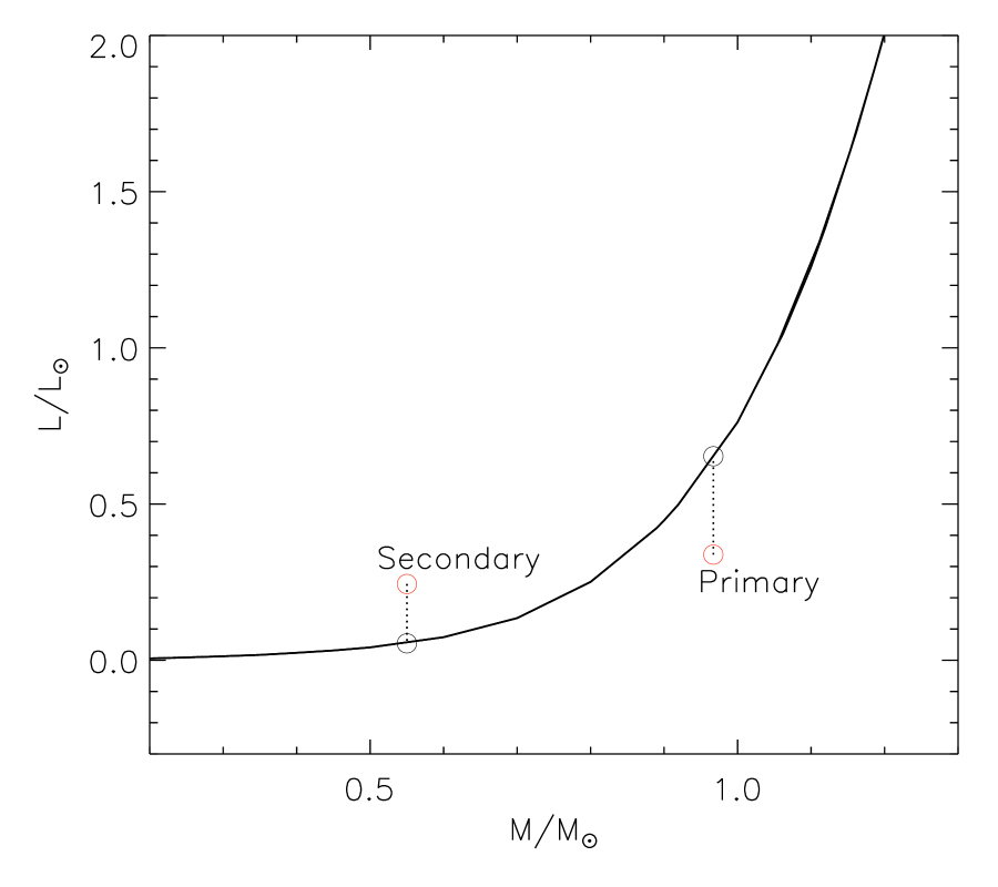
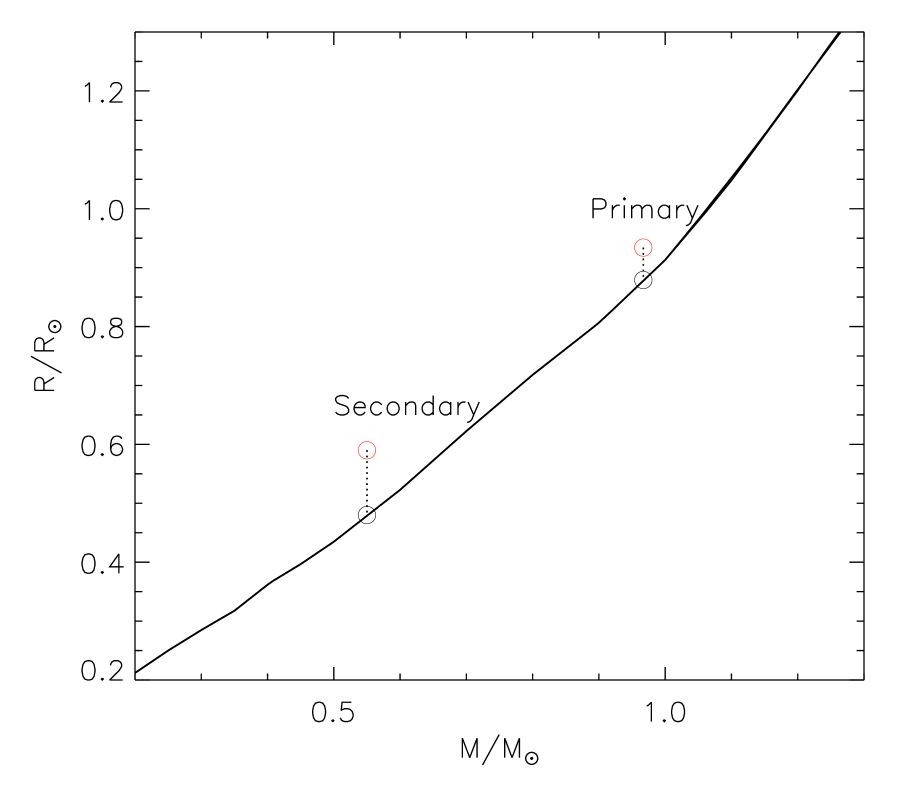
Figure 9: Locations of the components of EK Com on the main sequence mass-luminosity and mass-radius diagrams. The solid line represents 1 Gyr isochrones from Girardi et al. (2000) with solar chemical composition.

Table 4: Absolute parameters of EK Com

Parameter	Primary	Secondary
Mass ($M_{\odot}$)	0.967	0.338
Radius ($R_{\odot}$)	0.934	0.590
Luminosity ($L_{\odot}$)	0.550	0.243

We have also calculated the following parameters as described in Csizmadia and Klagyivik (2004): the bolometric luminosity ratio ($\lambda$), energy transfer parameters ($\beta$), $\beta_{\rm excess}$, $\beta_{\rm envelope}$, $\beta_{\rm corr}$, amount of the transferred luminosity ($\Delta L$). The values of the obtained parameters are given in Table 5.

Table 5: bolometric luminosity ratio, energy transfer parameters

$\lambda$	$\beta$	$\beta_{\rm excess}$	$\beta_{\rm envelope}$	$\beta_{\rm corr}$	$\Delta L$
0.417	0.711	0.005	0.706	0.704	0.159

5 Distance determination to EK Com

The standard $V$ magnitude of the comparison star is 12.060 (SA96). We now find the differential magnitude ($\Delta V$) between the variable and the comparison star at phases 0, 0.25, 0.50 and 0.75 respectively. From the spot fitted light curve, we find that $\Delta V=0.6594~{}(\Phi=0.0),\,0.0095~{}(\Phi=0.25),\,0.6451~{}(\Phi=0.50),\,0.0462~{}(\Phi=0.75)$. A brief magnitude calibration gives the standard magnitude of EK Com $V=12.719~{}(\Phi=0.0),12.069~{}(\Phi=0.25),\,12.705~{}(\Phi=0.50),\,12.106~{}(\Phi=0.75)$. With the derived luminosities for both the components and the bolometric correction values found from the temperatures of the components following Flower (1996), we obtain the absolute magnitudes of the components as 5.652 mag and 6.476 mag respectively. For the primary and secondary components, the bolometric correction values used are $-0.253$ and $-0.190$ respectively. The combined absolute magnitude of the system is then computed as $M_{\rm V}=5.235$ mag. On the other hand, Rucinski and Duerbeck (1997) derived the following empirical relation with an accuracy of $\pm 0.1$ to calculate the absolute magnitude of W UMa systems.

$$M_{V}=-4.44\,\log\,P+3.02(B-V)_{0}+0.12.$$ (6)

Using the above equation, the absolute magnitude of EK Com can be calculated as 5.000 mag. Our calculated value of the absolute magnitude of EK Com 5.235 mag is nearly 0.23 mag fainter than the value obtained from Eq. 6. We now take the visual magnitude $V=12.106$ at phase $\Phi=0.75$. The interstellar absorption is taken as $A_{V}=0.031$. The distance modulus of EK Com is then computed to be $(m-M)=6.840$ mag using our computed value of the absolute magnitude of 5.235 mag for the binary system. This corresponds to a distance of $233.346\rm~{}pc$ or parallax of $4.30\rm~{}mas$. On the other hand, if the value of the absolute magnitude of 5.000 mag obtained from Eq. 6 is used, the distance of EK Com can be calculated as $260.016$ pc or a parallax of $3.8$ mas.

6 Summary & Conclusions

We have presented a photometric solution for the eclipsing binary EK Com obtained from the new high-precision time-series CCD photometric observations with complete phase coverage in the V band. The new observations indicate that the star may be of A-type with a flat secondary minimum. By using the WD code, we have found that the system is a total-eclipsing binary star with an orbital inclination of $i[^{o}]=89.800\pm 0.075$ and a high degree of over-contact configuration 33.0%. The difference in the mean temperatures between the two components is found to be $141\pm 10~{}K$. The observed light curve is quite asymmetric, especially at quadrature levels, because of surface activity on either of the two components. This feature of the light curve is explained assuming a hot spot on the primary component.

It has been found that the photometric mass ratio determined from the WD light curve modelling approach is reliable for a totally eclipsing over-contact binary. Keeping in view of this fact, the absolute physical parameters of the two components are determined based on the results of the light curve solution and by the MV96 method. The luminosity of the star is calculated using the temperature and radius of each of the individual components. The photometric spot solutions given in Table 3 are tentative, as it has been observed that with the spot solutions included in the WD code, the whole light curve can be easily fitted, but a serious problem of uniqueness of the solution persists (Maceroni and van’t Veer, 1993) unless other means of investigation such as Doppler Imaging techniques are applied (Maceroni et al., 1994).

The spectroscopic radial velocity observations and long term photometric monitoring of the star is important to determine its actual type and to answer whether the deeper rounded shape of the primary eclipse seen in our observations is either due to the actual configuration of the system or due to its higher level of spot magnetic activity at different phases or both.

References

- Borovicka (1990) Borovicka, J., 1990. Journal of the American Association of Variable Star Observers (JAAVSO) 19, 8.
- Cox (2000) Cox, A. N., 2000. Allen’s astrophysical quantities.
- Csizmadia and Klagyivik (2004) Csizmadia, S., Klagyivik, P., 2004. A&A 426, 1001.
- Cutri et al. (2003) Cutri, R. M., Skrutskie, M. F., van Dyk, S., Beichman, C. A., Carpenter, J. M., Chester, T., Cambresy, L., Evans, T., Fowler, J., Gizis, J., Howard, E., Huchra, J., Jarrett, T., Kopan, E. L., Kirkpatrick, J. D., Light, R. M., Marsh, K. A., McCallon, H., Schneider, S., Stiening, R., Sykes, M., Weinberg, M., Wheaton, W. A., Wheelock, S., Zacarias, N., 2003. 2MASS All Sky Catalog of point sources.
- Flower (1996) Flower, P. J., 1996. ApJ 469, 355.
- Girardi et al. (2000) Girardi, L., Bressan, A., Bertelli, G., Chiosi, C., 2000. A&AS 141, 371.
- Kinman et al. (1966) Kinman, T. D., Wirtanen, C. A., Janes, K. A., 1966. ApJS 13, 379.
- Kwee and van Woerden (1956) Kwee, K. K., van Woerden, H., 1956. Bull. Astron. Inst. Netherlands 12, 327.
- Li and Zhang (2006) Li, L., Zhang, F., 2006. New Astronomy 11, 588.
- Lucy (1967) Lucy, L. B., 1967. Zeitschrift fur Astrophysik 65, 89.
- Maceroni and van’t Veer (1993) Maceroni, C., van’t Veer, F., 1993. A&A 277, 515.
- Maceroni and van’t Veer (1996) Maceroni, C., van’t Veer, F., 1996. A&A 311, 523. [MV96]
- Maceroni et al. (1994) Maceroni, C., Vilhu, O., van’t Veer, F., van Hamme, W., 1994. A&A 288, 529.
- Mochnacki (1981) Mochnacki, S. W., 1981. ApJ 245, 650.
- O’Connell (1951) O’Connell, D. J. K., 1951. Publications of the Riverview College Observatory 2, 85.
- Prša and Zwitter (2005) Prša, A., Zwitter, T., 2005. ApJ 628, 426.
- Ruciński (1969) Ruciński, S. M., 1969. Acta Astronomica 19, 245.
- Rucinski (2001) Rucinski, S. M., 2001. AJ 122, 1007.
- Rucinski and Duerbeck (1997) Rucinski, S. M., Duerbeck, H. W., 1997. PASP 109, 1340.
- Samec et al. (1996) Samec, R. G., Gray, J. D., Carrigan, B. J., 1996. The Observatory 116, 75. [SA96]
- Sandquist and Shetrone (2003) Sandquist, E. L., Shetrone, M. D., 2003. AJ 125, 2173.
- Schlegel et al. (1998) Schlegel, D. J., Finkbeiner, D. P., Davis, M., 1998. ApJ 500, 525.
- Schwarzenberg-Czerny (1996) Schwarzenberg-Czerny, A., 1996. ApJL 460, 107. [SC96]
- Stetson (1987) Stetson, P. B., 1987. PASP 99, 191.
- Stetson (1992) Stetson, P. B., 1992. More Experiments with DAOPHOT II and WF/PC Images. In: D. M. Worrall, C. Biemesderfer, & J. Barnes (Ed.), Astronomical Data Analysis Software and Systems I. Vol. 25 of Astronomical Society of the Pacific Conference Series. p. 297.
- van Hamme (1993) van Hamme, W., 1993. AJ 106, 2096.
- Wilson (1979) Wilson, R. E., 1979. ApJ 234, 1054.
- Wilson (1990) Wilson, R. E., 1990. ApJ 356, 613.
- Wilson and Devinney (1971) Wilson, R. E., Devinney, E. J., 1971. ApJ 166, 605.
- Zhang et al. (2005) Zhang, X. B., Zhang, R. X., Deng, L., 2005. AJ 129, 979.