Multiple-Relaxation-Time Lattice Boltzmann Approach to Compressible Flows with Flexible Specific-Heat Ratio and Prandtl Number

Abstract

A new multiple-relaxation-time lattice Boltzmann scheme for compressible flows with arbitrary specific heat ratio and Prandtl number is presented. In the new scheme, which is based on a two-dimensional $16$-discrete-velocity model, the kinetic moment space and the corresponding transformation matrix are constructed according to the seven-moment relations associated with the local equilibrium distribution function. In the continuum limit, the model recovers the compressible Navier-Stokes equations with flexible specific-heat ratio and Prandtl number. Numerical experiments show that compressible flows with strong shocks can be simulated by the present model up to Mach numbers $Ma\sim 5$.

1 Introduction

Over the last two decades, the Lattice Boltzmann (LB) method has become a prominent tool in computational fluid dynamics[1, 2, 3], with a broad spectrum of complex flows applications, ranging from multiphase flows[4, 5, 6], magnetohydrodynamics[7, 8, 9, 10], flows through porous media[11, 12, 13] and thermal fluid dynamics[14, 15], to cite but a few. Being based on a low-Mach expansion of Maxwell-Boltzmann local equilibria, standard LB models are typically used for the simulation of quasi-incompressible flows. Given the great importance of shock-wave dynamics in many fields of physics and engineering [16, 17], constructing LB models for high-speed compressible flows with shocks has been attempted since the early days of LB research. However, current LB versions for compressible flows are still subject to at least one of the following constraints: low Mach number, fixed Prandtl number and fixed specific heat ratio. Broadly speaking, to date, there are two LB approaches for the simulation of compressible flows. The first is based on the Single-Relaxation-Time (SRT) Bhatnagar-Gross-Krook (BGK) approximation[18], where the local equilibrium distribution function $f_{i}^{eq}$ is calculated from a truncated Taylor expansion of the flow velocity, where $i$ is the index of discrete velocity. Models along this line can be roughly categorized into two groups, the standard LB and the Finite Difference (FD) LB. Examples in the first group are referred to the works of Alexander and Chen et al.[19], Sun, et al.[20], Yan, et al. [21], and so on. In the FDLB formulation, space and time discretizations are independent, and to overcome the limit of low Mach number, one has to confine the LB to be a solver of Euler or Navier-Stokes (NS) equations. In such a case, the discrete $f_{i}^{eq}$ is best seen as a local attractor of the collisional relaxation process, leading to the desired form of the macroscopic moments. Examples are referred to the works of Tsutahara, et al[22, 23], Xu, et al[24], Shu, et al[25] and He, et al[26]. The application of BGK also leads to a fixed Prandtl number. In most existing models, the specific heat ratio is fixed to a nonrealistic constant because only the translational degrees of freedom are taken into account in the internal energy. The second way consists of resorting to the original scattering-matrix formulation of the LB equation[27], whose optimized version is nowadays known as Multiple-Relaxation-Time (MRT) LB scheme[28]. In the MRT-LB formulation, the collision step is first calculated in the kinetic moment space (KMS), i.e. the space spanned by the kinetic moments defined by the projection of the distribution function onto a basis set of $N$ Hermite polynomials. Subsequently, the streaming step is performed back in the discrete velocity space spanned by a suitable set of $N$ discrete velocities $\mathbf{v}_{i}$. In contrast to the SRT model, the MRT version caters for more adjustable parameters and degrees of freedom. The relaxation rates of the various kinetic moments due to particle collisions may be adjusted independently. This overcomes some obvious deficiencies of the SRT model, such as a fixed Prandtl number. The low-Mach number constraint is generally caused by the numerical instability problem. To this regard, extensive efforts have been made in the past years, such as the entropic method[29, 30, 31], the fix-up scheme[29, 32], Flux-limiters[33] and dissipation[24, 34] techniques. In many cases with low-speed flows, it has been shown [35] that the MRT LB model also offers enhanced numerical stability. As far as we know, nearly all existing MRT models have been focussing on the standard LB for isothermal systems without strong shocks.

Recently, we presented a thermal MRT FDLB model for high-speed compressible flows[36]. The MRT model uses $16$ discrete velocities, as suggested by Kataoka and Tsutahara[23] in the SRT version. In that MRT model, the KMS and corresponding transformation matrix are constructed according to the group representation theory; equilibria of the nonconserved moments are chosen so as to recover the compressible Navier-Stokes equations through the Chapman-Enskog analysis. Neither the formulation, nor the simulation procedure are by any means related to a truncated Taylor-expansion of local equilibrium distribution function $f_{i}^{eq}$. Consequently, the discrete local equilibrium $f_{i}^{eq}$ remains Maxwellian regardless of the value of the Mach number. However, the model is restricted to a nonphysical value of the specific-heat-ratio, $2$. For convenience of description, we will refer to that model as model $I$.

In this letter, we formulate a LB model II for compressible flows with arbitrary specific-heat-ratio. At variance with model I, at high-Mach number, the local equilibria of model II depart from a Maxwellian. Nevertheless, the method is able to simulate both low and high Mach numbers regimes (up to $Ma\sim 5$).

2 Brief review of the MRT LB model

According to the main strategy of the MRT-LB scheme, the differential form of the MRT-LB equation read as follows:

$$\frac{\partial f_{i}}{\partial t}+v_{i\alpha}\frac{\partial f_{i}}{\partial x_{\alpha}}=-\mathbf{M}_{il}^{-1}\hat{\mathbf{S}}_{lk}(\hat{f}_{k}-\hat{f}_{k}^{eq})\text{,}$$ (1)

where $\mathbf{v}_{i}$ is the discrete particle velocity, $i=1$,$\ldots$ ,$N$, $N$ is the number of discrete velocities, the subscript $\alpha$ indicates $x$ or $y$. The variable $t$ is time, $x_{\alpha}$ is the spatial coordinate. The matrix $\hat{\mathbf{S}}=\mathbf{MSM}^{-1}=diag(s_{1},s_{2},\cdots,s_{N})$ is the diagonal relaxation matrix, $f_{i}$ and $\hat{f}_{i}$ are the particle distribution function in the velocity space and the kinetic moment space respectively, $\hat{f}_{i}=m_{ij}f_{j}$, $m_{ij}$ is an element of the matrix $\mathbf{M}$. Obviously, the mapping between KMS and velocity space is defined by the linear transformation $\mathbf{M}$, i.e., $\hat{\mathbf{f}}=\mathbf{Mf}$, $\mathbf{f=M}^{-1}\hat{\mathbf{f}}$, where the bold-face symbols denote N-dimensional column vectors, e.g., $\mathbf{f}=(f_{1},f_{2},\cdots,f_{N})^{T}$, $\hat{\mathbf{f}}=(\hat{f}_{1},\hat{f}_{2},\cdots,\hat{f}_{N})^{T}$, $\mathbf{M}=(m_{1},m_{2},\cdots,m_{N})^{T}$, $m_{i}=(m_{i1},m_{i2},\cdots,m_{iN})$. $\hat{f}_{i}^{eq}$ is the equilibrium value of the moment $\hat{f}_{i}$. The equation reduces to the usual lattice BGK equation if all the relaxation parameters are set to be a single relaxation time $\tau$, namely $\hat{\mathbf{S}}=\frac{1}{\tau}\mathbf{I}$, where $\mathbf{I}$ is the identity matrix.

3 Construction of energy-conserving MRT LB model

We use the two-dimensional discrete velocity model by Kataoka and Tsutahara (see Fig. 1), which reads as follows:

$$(v_{ix,}v_{iy})=\left\{\begin{array}[]{cc}\mathbf{cyc}:(\pm 1,0),&\text{for }1\leq i\leq 4,\\ \mathbf{cyc}:(\pm 6,0),&\text{for }5\leq i\leq 8,\\ \sqrt{2}(\pm 1,\pm 1),&\text{for }9\leq i\leq 12,\\ \frac{3}{\sqrt{2}}(\pm 1,\pm 1),&\text{for }13\leq i\leq 16,\end{array}\right.$$

where cyc indicates the cyclic permutation. The $16$ velocities are grouped into four energy levels, $v^{2}$, where $v=1,2,3,6$. In this model, besides the translational degrees of freedom, a parameter $\eta_{i}$ is introduced, in order to describe the $(b-2)$ extra-degrees of freedom corresponding to molecular rotation and/or vibration, where $\eta_{i}=5/2$ for $i=1$, $\cdots$,$4$, and $\eta_{i}=0$ for $i=5$, $\cdots$, $16$. Details are referred to the original publication[23]. In our simulations, the time evolution is based on the usual first-order upwind scheme, while space discretization is performed through a Lax-Wendroff scheme.

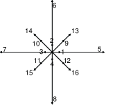
Figure 1: Distribution of $\mathbf{v}_{i}$ for the discrete velocity model.

The moment representation provides a convenient way to express collisional relaxation on different time scales for the various kinetic moments. However, the choice of the kinetic moments is not unique. They can be identified with physical quantities, such as density, momentum, energy, momentum and energy fluxes, and so on. Inspired by a close tie with tensor Hermite polynomials, many researchers choose the moments according to the monomials of Cartesian components of the discrete velocities $v_{ix}^{m}v_{iy}^{n}$, $m,n=0,1,2,\cdots$[35]. In this Letter, the KMS and equilibria of the moments are chosen according to the seven-moment relations (Equations (5a-5g) in Reference [23]), associated with the local equilibrium distribution function $f_{i}^{eq}$(Equation (8) in Reference [23]), which is a polynomial of the flow velocity up to the third order. The incorporation of the parameter $b$ permits to tune the specific-heat-ratio, $\gamma=(b+2)/b$.

The right-hand-sides of the seven equations indicate seven monomials, $1$, $v_{i\alpha}$, $(v_{i\alpha}^{2}+\eta_{i}^{2})$, $v_{i\alpha}v_{i\beta}$, $(v_{i\beta}^{2}+\eta_{i}^{2})v_{i\alpha}$, $v_{i\alpha}v_{i\beta}v_{i\chi}$, $(v_{i\chi}^{2}+\eta_{i}^{2})v_{i\alpha}v_{i\beta}$. In order to make the choice of moments more transparent, we construct the transformation matrix through a simple combination of the seven monomials above (see Appendix for details). As a result, at least eight of these moments carry an explicit physical meaning: $\hat{f}_{1}=m_{1i}f_{i}$ is the fluid density; $\hat{f}_{2}=m_{2i}f_{i}$ and $\hat{f}_{3}=m_{3i}f_{i}$ correspond to the $x-$ and $y-$ components of momentum (mass flux); $\hat{f}_{4}=m_{4i}f_{i}$ corresponds to the total energy mode; $\hat{f}_{6}=m_{6i}f_{i}$ and $\hat{f}_{7}=m_{7i}f_{i}$ correspond to the diagonal and off-diagonal components of the stress tensor; $\hat{f}_{8}=m_{8i}f_{i}$ and $\hat{f}_{9}=m_{9i}f_{i}$ correspond to the $x-$ and $y-$ components of the total energy flux.

At variance with previous MRT models[35, 37], the transformation matrix $\mathbf{M}$ used in this work is not based upon a Gram-Schmidt orthogonalization procedure. This is because such a procedure does not lead to a conserved energy, as required for a consistent thermal and compressible model. The moments can be divided into two groups. The first group consists of those which are locally conserved in the collision process, i.e. $\hat{f}_{i}=\hat{f}_{i}^{eq}$. There are four such conserved moments, density $\rho$, momenta $j_{x}$, $j_{y}$, and energy $e$ in two dimensions, which are denoted by $\hat{f}_{1}$, $\hat{f}_{2}$, $\hat{f}_{3}$, $\hat{f}_{4}$ mentioned above, respectively. The second group consists of the non-conserved ones, i.e. $\hat{f}_{i}\neq\hat{f}_{i}^{eq}$. The equilibria of the non-conserved moments are functionals of the conserved ones. For the collision process, one has maximum freedom in the construction of the equilibrium functions of the non-conserved moments, provided the basic principles of physics are satisfied (conservations of mass, momentum and energy). In this model, the corresponding equilibrium distribution functions in the KMS $\hat{f}_{i}^{eq}$ are chosen according to the seven-moment relations, too (see Appendix). By using the Chapman-Enskog expansion[38] on the two sides of the LB equation, the final NS equations for compressible fluids read as follows:

$$\frac{\partial\rho}{\partial t}+\frac{\partial j_{x}}{\partial x}+\frac{\partial j_{y}}{\partial y}=0,$$ (2a)

$$\frac{\partial j_{x}}{\partial t}+\frac{\partial}{\partial x}\left(\frac{j_{x}^{2}}{\rho}\right)+\frac{\partial P}{\partial x}+\frac{\partial}{\partial y}\left(\frac{j_{x}j_{y}}{\rho}\right)$$ (2b)

$$= \frac{\partial}{\partial x}[\rho RT(\frac{(b-2)D}{bs_{5}}+\frac{d}{s_{6}})]+\frac{\partial}{\partial y}\frac{\rho RTs_{xy}}{s_{7}}\text{,}$$

$$\frac{\partial j_{y}}{\partial t}+\frac{\partial}{\partial x}\left(\frac{j_{x}j_{y}}{\rho}\right)+\frac{\partial}{\partial y}\left(\frac{j_{y}^{2}}{\rho}\right)+\frac{\partial P}{\partial y}$$ (2c)

$$= \frac{\partial}{\partial y}[\rho RT(\frac{(b-2)D}{bs_{5}}-\frac{d}{s_{6}})]+\frac{\partial}{\partial x}\frac{\rho RTs_{xy}}{s_{7}}\text{,}$$

$$\frac{\partial e}{\partial t}+\frac{\partial}{\partial x}[(e+2P)j_{x}/\rho]+\frac{\partial}{\partial y}[(e+2P)j_{y}/\rho]$$ (2d)

$$= 2\frac{\partial}{\partial x}\{\frac{\rho RT}{s_{8}}[(\frac{b}{2}+1)R\frac{\partial T}{\partial x}+s_{xy}u_{y}+(2\frac{\partial u_{x}}{\partial x}-\frac{2}{b}D)u_{x}]\}$$

$$+2\frac{\partial}{\partial y}\{\frac{\rho RT}{s_{9}}[(\frac{b}{2}+1)R\frac{\partial T}{\partial y}+s_{xy}u_{x}$$

$$+(2\frac{\partial u_{y}}{\partial y}-\frac{2}{b}D)u_{y}]\}\text{,}$$

where $$P=\rho RT e=b\rho RT+j_{\alpha}^{2}/\rho s_{xy}\equiv(\partial_{x}u_{y}+\partial_{y}u_{x}) D\equiv(\partial_{x}u_{x}+\partial_{y}u_{y}) d\equiv(\partial_{x}u_{x}-\partial_{y}u_{y}) s_{5},s_{6},s_{7} s_{8},s_{9} s_{8}=s_{9} \hat{\mathbf{S}} \hat{\mathbf{f}} \hat{\mathbf{f}}^{eq} \rho j_{x} j_{y} e s_{1},s_{2},s_{3},s_{4} [0,1/dt] s_{5}=s_{6}=s_{7}=s_{8}=s_{9}=s$$, is twice the total energy, , , and , are related to viscosity, are related to heat conductivity. The relaxation parameters are not completely independent, since the isotropy constraints impose coupling between some of these relaxation parameters, e.g., . Since the elements of represent the inverse of the relaxation time for to its equilibrium in KMS, and the values of , , , and are conserved in the relaxation process, the values of can be fine-tuned independently. The remaining relaxation parameters must belong to the interval for reasons of linear stability. In the limit , the above NS equations reduce to the SRT compressible NS equations.

4 Numerical Simulation and Analysis

In this section we study the following problems using the new MRT LB model: measure of the sound speed, one- and two-dimensional Riemann problems, Richtmyer-Meshkov instability. We work in a frame where the constant $R=1$.

(a) Speed of sound

In order to validate the proposed model, the sound speed is calculated and compared to the theoretical value $c_{s}=\sqrt{\gamma T}$ [22]. A one-dimensional tube is used. In the tube, a plate divides the fluids, that share the same temperature and feature a small difference in pressure ($p_{1}/p_{2}=1.0+10^{-10}$) at the initial stage. The pressure ratio is so small that expansion and compression waves propagate at the sound speed in both directions when the plate is removed. The position of the pressure jump is measured to calculate the speed of sound. The results at various temperature levels are shown in Fig. 2, and the calculated values are found to agree well with the theoretical ones.

Figure 2: Calculation results and theoretical values of sound speed.

(b) One-dimensional Riemann problem

Here, the two-dimensional model is used to solve the one-dimensional Riemann problem, so as to visually show the advantages of this model as compared to its SRT version. Consider the Riemann problem with initial condition given by

$$\begin{array}[]{cc}(\rho,u_{1},u_{2},T)|_{L}=(5.99924,19.5975,0.0,76.8254)\text{,}&\\ (\rho,u_{1},u_{2},T)|_{R}=(5.99242,-6.19633,0.0,7.69222)\text{,}&\end{array}$$

where subscript “L” and “R” indicate the left and right macroscopic variables of discontinuity. The numerical and exact solutions for two different specific-heat ratios $\gamma=7/5$ and $\gamma=5/3$ at time $t=0.13$ are shown in Fig.3, where the common parameters for SRT and MRT simulations are $dx=dy=0.002$, $dt=10^{-6}$. The relaxation time in SRT is $\tau=10^{-5}$, while the collision parameters in MRT are $s_{5}=5\times 10^{3}$, $s_{6}=10^{4}$, and other values of $s$ are $10^{5}$. In the $x$ direction, $f_{i}=f_{i}^{eq}$ is set on the boundary nodes before the disturbance reaches the two ends. The equilibrium distribution function $f_{i}^{eq}$ in velocity space can be obtained via the linear transformation, $\mathbf{f^{eq}=M}^{-1}\hat{\mathbf{f}}^{eq}$. Along the $y$ direction, periodic boundary conditions are adopted. The red triangle and red circle symbols correspond to MRT simulation results with $\gamma=7/5$ and $\gamma=5/3$, respectively; the green triangle and green circle symbols correspond to SRT simulation results with $\gamma=7/5$ and $\gamma=5/3$, respectively; the solid lines represent the exact solutions for the case $\gamma=7/5$, and the dashed lines represent the exact solutions for $\gamma=5/3$. We find that the oscillations at the discontinuity are weaker in MRT simulations than in their SRT countrepart. This shows that the problematic “wall-heating" phenomenon is weaker in the MRT model than in its SRT version.

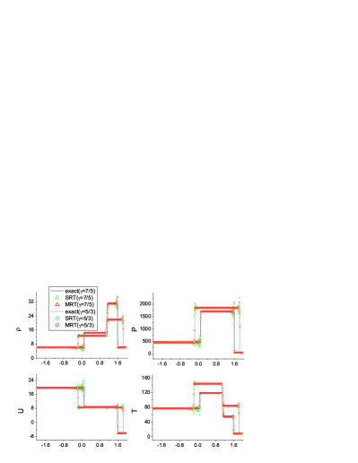
Figure 3: The numerical and exact solutions for the one-dimensional Riemann problem at time $t=0.13$.

(c) Two-dimensional Riemann problem

Compared with the relatively simple 1-D configurations, the 2-D Riemann problem consists of a plethora of geometric wave patterns that pose a challenge for the simulation. In two-dimensions, the Riemann problem consists of four uniform states in each quadrant, $(\rho,u_{1},u_{2},T)(x,y,0)=(\rho_{i},u_{1i},u_{2i},T_{i}),i=1,2,3,4$, where $i$ denotes the $i$th quadrant. We solve the 2-D Riemann problem with initial data as follows:

$$\begin{array}[]{c}\rho_{1}=1.5\text{,}u_{11}=0\text{,}u_{21}=0\text{,}T_{1}=1\text{;}\\ \rho_{2}=0.5323\text{,}u_{12}=1.206\text{,}u_{22}=0\text{,}T_{2}=0.3/0.5323\text{;}\\ \rho_{3}=0.138\text{,}u_{13}=1.206\text{,}u_{23}=1.206\text{,}T_{3}=0.029/0.138\text{;}\\ \rho_{4}=0.5323\text{,}u_{14}=0\text{,}u_{24}=1.206\text{,}T_{4}=0.3/0.5323\text{.}\end{array}$$

Figure 4 shows the density contours of the 2-D Riemann problem by MRT LB simulation at time $t=0.12$, where the parameters are $dx=dy=0.002$, $dt=10^{-5}$, $s_{8}=s_{9}=2\times 10^{4}$, other values of $s$ are $3\times 10^{3}$. The Mach number of the second and fourth quadrants are $1.358$, and the third quadrant is $3.1444$. While the SRT version is found to fail, the MRT LB successfully recovers the main features observed in earlier computations [39, 40].

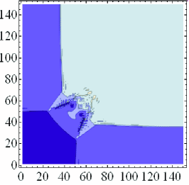
Figure 4: (Color online) Density contour lines of the 2-D Riemann problem in MRT LB simulation at time $t=0.12$. From purple to gray, the density value increases.

(d) Richtmyer - Meshkov instability

Studies of the shock-induced Richtmyer - Meshkov (RM) instability are of great importance from both viewpoints of fundamental research and practical applications. For example, the RM instability occurs in Inertial Confined Fusion, Scramjet engine, supersonic and hypersonic combustion, and others. In addition, it also plays an important role in some natural phenomena, such as Supernova explosions, formation of salt domains, and others. Although most practical problems are three-dimensional, 2D studies are also of recognized value, as they offer useful insights into the basic physics of these problems. The simulation of RM instability still remains a challenging topic to this day.

The initial configuration of our simulation is illustrated in Fig. 5(a), where an interface with sinusoidal perturbation separates two different fluids and a incident shock wave, with the Mach number $2.5$, traveling from the right side, hits the interface immediately. The computational domain is a rectangle with length $0.36$ and height $0.1$, which is divided into $360\times 100$ mesh-cells. The initial sinusoidal perturbation at the interface is: $x=0.24+0.005\times\sin(\pi/2+40\pi y)$, where the cycle of initial perturbation is $0.05$, and the amplitude is $0.005$. The initial conditions are as follows:

$$\left\{\begin{array}[]{cc}(\rho,u_{1},u_{2},p)_{l}=(0.1358,0,0,1)\text{,}&\\ (\rho,u_{1},u_{2},p)_{m}=(1,0,0,1)\text{,}&\\ (\rho,u_{1},u_{2},p)_{r}=(3.33333,-2.07063,0,7.125)\text{,}&\end{array}\right.$$

where the subscripts $l$, $m$, $r$ indicate the left, middle, right regions of the whole domain. The following boundary conditions are imposed: (1) inflow at the right side; (2) reflecting condition at the left boundary, and (3) periodic boundary conditions are applied at the top and bottom boundaries. The reflecting boundary condition implies that the $x$ component of the fluid velocity on the boundary is the reverse of the one of the mirror-image interior point. The parameters are as follows: $\gamma=1.4$, $dt=10^{-5}$, $s_{5}=2\times 10^{3}$, and $10^{5}$ for the others.

When the shock wave passes the interface from the right, a reflected rarefaction wave to the right and a transmission wave to the left, are generated, and the perturbation amplitude decreases with the interface motion to the left (Figure 5 (b)). Then, the peak and valley of initial interface invert, the heavy and light fluids gradually penetrate into each other as time goes on, the light fluid “rises" to form a bubble and the heavy fluid “falls" to generate a spike ( shown in Figure 5 (c)). The transmission wave reaches the solid wall on the left and reflects to the right, encounters the interface again, converts into a transmission wave penetrating into the heavy fluid zone and a reflection wave back to the light fluid. Before the second shock wave reaches the interface, the interface continues to move, and the disturbance develops at a lower growth rate. When the second shock reaches the interface, the instability growth rate of the disturbance significantly enhances. The disturbance of the interface continues to grow, eventually forming a mushroom shape (Figure 5 (d)). The simulation results show a satisfactory agreement with those of other numerical simulations [41, 42] and experiments[43, 44]. In the experimental study of Puranik et al.[43] the shock wave travels from light (air) to heavy ($CO_{2}$) medium, while the reverse is true in our simulation. As a result, interface reversals are observed in our simulation. The same mechanism is also mentioned in Ref. [43] (see Fig. 11 in [43]), which is a typical characteristic of an incident shock from the heavier to the lighter material. Even though the region with light medium is a cylindrical bubble in their experiments, while it is a rectangle with distortions in our simulation, the experiments on the interaction of a shock wave with a single cylindrical bubble [44] also show high similarity with our simulation results, both in terms of the reversal mechanism and of the mushroom shape.

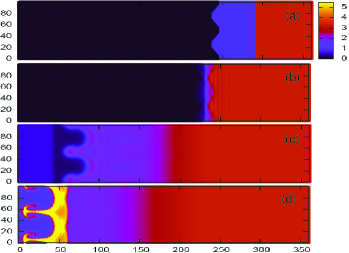
Figure 5: (Color online) Snapshots of RM instability: density contour lines at times $t=0$, $t=0.02$, $t=0.074$, $t=0.104$, respectively. From blue to red the color corresponds to the increasing of density.

5 Conclusions and remarks

In this Letter, we have proposed a MRT-FDLB model for compressible flows with flexible specific heat ratio and Prandtl number, as appropriate for most applications. Different transport coefficients, such as viscosity and heat conductivity, are related to different collision parameters, thereby allowing a separate control of the different transport processes. The new scheme has been validated for a series of one and two-dimensional numerical benchmarks, always showing satisfactory agreement with theoretical results and previous numerical work. Three-dimensional extensions of the present scheme appear conceptually straightforward and shall make the object of future work.

A. Xu and G. Zhang acknowledge support of the Science Foundations of LCP and CAEP[under Grant Nos. 2009A0102005, 2009B0101012], National Natural Science Foundation of China [under Grant Nos. 10775018, 10702010]. F. Chen and Y. Li acknowledge support of National Basic Research Program of China [under Grant No. 2007CB815105].

6 Appendix. Construction of the transformation matrix and $\hat{f}_{i}^{eq}$

In order to construct the transformation matrix in KMS, we take the monomial $v_{i\alpha}v_{i\beta}$ as an example. Three possibilities arise: (a) $\alpha=\beta=x$, $v_{i\alpha}v_{i\beta}=v_{ix}^{2}$, (b) $\alpha=\beta=y$, $v_{i\alpha}v_{i\beta}=v_{iy}^{2}$, (c) $\alpha=x$, $\beta=y$, $v_{i\alpha}v_{i\beta}=v_{ix}v_{iy}$. “(a)+(b)" gives $(v_{ix}^{2}+v_{iy}^{2})$, “(a)-(b)" gives $(v_{ix}^{2}-v_{iy}^{2})$. In this way, the transformation matrix can be composed as follows: $\mathbf{M}=(m_{1},m_{2},\cdots,m_{16})^{T}$, where $m_{1i}=1\text{,}\qquad m_{2i}=v_{ix}\text{,}\qquad m_{3i}=v_{iy}\text{,}\qquad m_{4i}=v_{ix}^{2}+v_{iy}^{2}+\eta_{i}^{2}\text{,}\qquad m_{5i}=v_{ix}^{2}+v_{iy}^{2}\text{,}\qquad m_{6i}=v_{ix}^{2}-v_{iy}^{2}\text{,}\qquad m_{7i}=v_{ix}v_{iy}\text{,}\qquad m_{8i}=v_{ix}(v_{ix}^{2}+v_{iy}^{2}+\eta_{i}^{2})\text{,}\qquad m_{9i}=v_{iy}(v_{ix}^{2}+v_{iy}^{2}+\eta_{i}^{2})\text{,}\qquad m_{10i}=v_{ix}(v_{ix}^{2}+v_{iy}^{2})\text{,}\qquad m_{11i}=v_{iy}(v_{ix}^{2}+v_{iy}^{2})\text{,}\qquad m_{12i}=v_{ix}(v_{ix}^{2}-v_{iy}^{2})\text{,}\qquad m_{13i}=v_{iy}(v_{ix}^{2}-v_{iy}^{2})\text{,}\qquad m_{14i}=(v_{ix}^{2}+v_{iy}^{2})(v_{ix}^{2}+v_{iy}^{2}+\eta_{i}^{2})\text{,}\qquad m_{15i}=v_{ix}v_{iy}(v_{ix}^{2}+v_{iy}^{2}+\eta_{i}^{2})\text{,}\qquad m_{16i}=(v_{ix}^{2}-v_{iy}^{2})(v_{ix}^{2}+v_{iy}^{2}+\eta_{i}^{2})\text{,}$ where $i=1,\cdots,16$.

The corresponding equilibrium distribution functions in KMS are as follows: $\hat{f}_{1}^{eq}=\rho\text{,}\qquad\hat{f}_{2}^{eq}=j_{x}\text{,}\qquad\hat{f}_{3}^{eq}=j_{y}\text{,}\qquad\hat{f}_{4}^{eq}=e\text{,}\qquad\hat{f}_{5}^{eq}=2P+(j_{x}^{2}+j_{y}^{2})/\rho\text{,}\qquad\hat{f}_{6}^{eq}=(j_{x}^{2}-j_{y}^{2})/\rho\text{,}\qquad\hat{f}_{7}^{eq}=j_{x}j_{y}/\rho\text{,}\qquad\hat{f}_{8}^{eq}=(e+2P)j_{x}/\rho\text{,}\qquad\hat{f}_{9}^{eq}=(e+2P)j_{y}/\rho\text{,}\qquad\hat{f}_{10}^{eq}=(4P+j_{x}^{2}/\rho+j_{y}^{2}/\rho)j_{x}/\rho\text{,}\qquad\hat{f}_{11}^{eq}=(4P+j_{x}^{2}/\rho+j_{y}^{2}/\rho)j_{y}/\rho\text{,}\qquad\hat{f}_{12}^{eq}=(2P+j_{x}^{2}/\rho-j_{y}^{2}/\rho)j_{x}/\rho\text{,}\qquad\hat{f}_{13}^{eq}=(-2P+j_{x}^{2}/\rho-j_{y}^{2}/\rho)j_{y}/\rho\text{,}\qquad\hat{f}_{14}^{eq}=2(b+2)\rho R^{2}T^{2}+(6+b)RT(j_{x}^{2}+j_{y}^{2})/\rho+(j_{x}^{2}+j_{y}^{2})^{2}/\rho^{3}\text{,}\qquad\hat{f}_{15}^{eq}=[(b+4)P+(j_{x}^{2}+j_{y}^{2})/\rho]j_{x}j_{y}/\rho^{2}\text{,}\qquad\hat{f}_{16}^{eq}=[(b+4)P+(j_{x}^{2}+j_{y}^{2})/\rho](j_{x}^{2}-j_{y}^{2})/\rho^{2}$.

References

- [1] \NameSucci S. \BookThe Lattice Boltzmann Equation for Fluid Dynamics and Beyond \PublOxford University Press, New York \Year2001.
- [2] \NameBenzi R., Succi S. and Vergassola M. \REVIEWPhys. Rep. 222 1992 145
- [3] \NameC. Aidun, J. Clausen \REVIEWAnnu. Rev. Fluid Mech. 42 2010 439
- [4] \NameShan X., Chen H. \REVIEWPhys. Rev. E4719931815; \REVIEWPhys. Rev. E4919942941.
- [5] For example, see \NameGonnella G., Orlandini E., and Yeomans J. M. \REVIEWPhys. Rev. Lett.7819971695; \NameMarenduzzo D., Orlandini E., and Yeomans J. M. \REVIEWPhys. Rev. Lett.982007118102.
- [6] \NameXu A.G., Gonnella G., Lamura A. \REVIEWPhys. Rev. E672003056105; \REVIEWibid742006011505; \NameXu A.G., Gonnella G., Lamura A., Amati G. and Massaioli F. \REVIEWEurophys. Lett.712005651.
- [7] \NameChen S., Chen H., Martinez D., and Matthaeus W. \REVIEWPhys. Rev. Lett.6719913776.
- [8] \NameSucci S., Vergassola M. and Benzi R. \REVIEWPhys. Rev. A4319914521.
- [9] \NameSchaffenberger W. and Hanslmeier A. \REVIEWPhys. Rev. E662002046702.
- [10] \NameBreyiannis G. and Valougeorgis D. \REVIEWPhys. Rev. E692004065702(R).
- [11] \NameGunstensen A. and Rothman D. H. \REVIEWJ. Geophy. Research9819936431.
- [12] \NameKang Q. J., Zhang D. X., and Chen S. Y. \REVIEWPhys. Rev. E662002056307.
- [13] \NameCali’ A., Succi S, Cancelliere A., Benzi R., and Gramignani M. \REVIEWPhys. Rev. A4519925771.
- [14] \NameAlexander F. J., Chen S., and Sterling J. D. \REVIEWPhys. Rev. E471993R2249.
- [15] \NameChen Y., Ohashi H., and Akiyama M. \REVIEWJ. Sci. Comp.121997169.
- [16] \NameWu C. C. and Roberts P.H. \REVIEWPhys. Rev. Lett7019933424; \NameSalomons E. and Mareschal M. \REVIEWPhys. Rev. Lett691992269; \NameKlein R., CF Mc Kee and Colella P. \REVIEWApJ.4201994213.
- [17] \NameXu A.G., Pan X. F., Zhang G.C. and Zhu J.S. \REVIEWJ. Phys.:Condens. Matter192007326212; \NameXu A. G., Zhang G. C., Pan X. F., Zhang P. and Zhu J.S. \REVIEWJ. Phys. D: Appl. Phys.422009075409.
- [18] \NameBhatnagar P., Gross E. P., and Krook M. K. \REVIEWPhys. Rev.941954511.
- [19] \NameAlexander F. J., Chen H., Chen S. and Doolen G. D. \REVIEWPhys. Rev. A4619921967.
- [20] \NameSun C. H. \REVIEWPhys. Rev. E5819987283; \NameSun C. and Hsu A.T. \REVIEWPhys. Rev. E682003016303.
- [21] \NameYan G. W., Chen Y. S. and Hu S. X. \REVIEWPhys Rev E591999454.
- [22] \NameWatari M. and Tsutahara M. \REVIEWPhys. Rev. E672003036306; \REVIEWPhys. Rev. E702004016703.
- [23] \NameKataoka T. and Tsutahara M. \REVIEWPhys. Rev. E692004035701(R).
- [24] \NamePan X.F., Xu A.G., Zhang G.C., Jiang S. \REVIEWInt. J. Mod. Phys. C1820071747; \NameGan Y.B., Xu A.G., Zhang G.C., Yu X., Li Y.J. \REVIEWPhysica A38720081721.
- [25] \NameQu K., Shu C., and Chew Y. T. \REVIEWPhys. Rev. E752007036706.
- [26] \NameWang Y., He Y. L., Zhao T. S., Tang G. H. and Tao W. Q. \REVIEWInt. J. Mod. Phys. C1820071961; \NameLi Q., He Y. L., Wang Y., and Tao W. Q. \REVIEWPhys. Rev. E762007056705.
- [27] \NameHiguera F. J., Succi S. and Benzi R. \REVIEWEurophys. Lett.91989345; \NameHiguera F. J. and Jimenez J. \REVIEWEurophys. Lett.91989662.
- [28] d’Humières D., Generalized lattice-Boltzmann equations, in Rarefied Gas Dynamics: Theory and Simulations, Vol. 159(AIAA Press, Washington, DC, 1992), pp450-458.
- [29] \NameAnsumali S., Karlin I. V. \REVIEWJ. Stat. Phys.1072002291.
- [30] \NameTosi F., Ubertini S., Succi S., Chen H., Karlin I.V. \REVIEWMath.Comput. Simul.722006227.
- [31] B. Boghosian, P. Love, P.V. Coveney, I.V. Karlin, S. Succi, J. Yepez, \REVIEWPhys. Rev. E, 68, 2003 025103R.
- [32] \NameLi Y., Shock R., Zhang R., Chen H. \REVIEWJ. Fluid Mech.5192004273.
- [33] \NameSofonea V., Lamura A., Gonnella G., Cristea A. \REVIEWPhys. Rev. E 702004046702.
- [34] \NameBrownlee R. A., Gorban A. N., Levesley J. \REVIEWPhys. Rev. E752007036711.
- [35] \NameLallemand P., and Luo L. S. \REVIEWPhys. Rev. E6120006546; \REVIEWPhys. Rev. E682003036706.
- [36] \NameChen F., Xu A. G., Zhang G. C., Li Y. J. arXiv:0908.3749(Submitted to PRE).
- [37] \NameAdhikari R., Succi S. \REVIEWPhys. Rev. E782008066701.
- [38] \NameMcCracken M. E., and Abraham J. \REVIEWPhys. Rev. E712005036701.
- [39] \NameLax P.D.,Liu X.D. \REVIEWSIAM J.Sci.Comput.191998319.
- [40] \NameKurganov A., Tadmor E. \REVIEWMeth. Part. Diff. Eq.182002584.
- [41] \NameLatini M., Schilling O., Don W. S. \REVIEWJ.Comput.Phys.2212007805.
- [42] \NameAnuchina N. N., Volkov V. I., Gordeychuk V. A., Es’kov N. S., Ilyutina O. S., Kozyrev O. M. \REVIEWJ. Comput. Appl. Math.168200411.
- [43] \NamePuranik P.B., Oakley J.G., Anderson M.H., Bonazza R. \REVIEWShock Waves132004413.
- [44] \NameHaas J. F., Sturtevant B. \REVIEWJ. Fluid Nech.181198741.