Imaging mesoscopic nuclear spin noise with a diamond magnetometer

Abstract

Magnetic Resonance Imaging (MRI) can characterize and discriminate among tissues using their diverse physical and biochemical properties. Unfortunately, submicrometer screening of biological specimens is presently not possible, mainly due to lack of detection sensitivity. Here we analyze the use of a nitrogen-vacancy center in diamond as a magnetic sensor for nanoscale nuclear spin imaging and spectroscopy. We examine the ability of such a sensor to probe the fluctuations of the ‘classical’ dipolar field due to a large number of neighboring nuclear spins in a densely protonated sample. We identify detection protocols that appropriately take into account the quantum character of the sensor and find a signal-to-noise ratio compatible with realistic experimental parameters. Through various example calculations we illustrate different kinds of image contrast. In particular, we show how to exploit the comparatively long nuclear spin correlation times to reconstruct a local, high-resolution sample spectrum.

I Introduction

Physical tools have historically facilitated advances in biology; notable examples are X-rays crystallography, DNA sequencing, microarrays techniques, and, above all, microscopy in its various forms. Extending Nuclear Magnetic Resonance (NMR) to the micro- and nano-scale promises to become another leading resource in the microscopist’s toolbox: Unlike any other technique, NMR is unique in allowing the generation of images with different information content. Multidimensional high-resolution spectroscopy is today routinely used in the liquid and solid state to unveil complex molecular structures, and this capability could prove groundbreaking if samples having sub-microscopic dimensions could be efficiently probed. Unfortunately, these features cannot be fully exploited at present because NMR lacks the sensitivity essential to high-resolution screening. The origin of this limitation is twofold: First, in “conventional” NMR the signal to noise ratio ($SNR$) is proportional to the nuclear magnetic polarization of the sample, which represents only a small fraction of the attainable maximum ($\sim 10^{-4}$ for protons in a 14 T magnet at 300 K). Second, Faraday induction is a poor detection method since, even with maximum polarization, the minimum number of spins needed to induce a measurable signal is comparatively large.

Although experiments performed at lower temperatures and/or higher fields can partly mitigate these problems, other more efficient detection techniques have recently been proposed. One strategy is to use the spin associated to a single nitrogen-vacancy (NV) center in diamond as a local magnetic field probe.Taylor08 ; Degen08 . The operating principles of this approach closely mimic those of an atomic vapor magnetometer Budker07 , where the applied magnetic field is inferred from the shift in the Larmor precession frequency. Owing to the exceptionally long coherence times of NV centers—exceeding 1 ms at room temperature in ultra-pure bulk samples Balasubramanian09 —detection of 3 nT over a measurement time of only 100 s has been experimentally demonstrated.Maze08 Further, a NV center within a diamond nanocrystal attached to an AFM tip was recently used to image a magnetic nanostructure with 20 nm resolution.Balasubramanian08

Here we focus on applications of a NV center mounted on a scanning probe for monitoring adjacent nuclear spins in an external, infinitely-extended organic sample. Rather than detecting single nuclear spins—an extremely challenging goal—we focus on the case where the NV center interacts with large ensembles of nuclear spins localized over effective volumes of $\sim$(10-50nm)³. This regime lends itself to a simplified description that simultaneously takes into consideration the quantum nature of the sensor—the NV center—while relying on a classical description of the long-range dipolar fields induced by the nuclear spin ensemble. Similar to prior magnetic resonance force microscopy experimentsDegen07 , our strategy exploits the small dimensions of the effective sample to probe the ‘nuclear spin noise’—i.e., the statistical fluctuations of the nuclear magnetization—rather than the magnetization itself. An important consequence is that, unlike traditional MRI, spatial resolution is not due to strong magnetic field gradients but is rather determined by the distance between the NV center and the sample. Assuming a very small external magnetic field we determine the conditions required for 2D nuclear spin imaging at (or near) room temperature, and show them to be compatible with realistic experimental parameters. Further, we show that, in addition to determining the local nuclear spin density, this strategy allows one to explore different kinds of contrast mechanisms (nearly a requisite when imaging, for example, densely protonated organic/biological systems). In particular, we show how to reconstruct the local nuclear spin correlation function and, from it, a spatially-resolved nuclear spin spectrum.

The paper is organized as follows. First, we briefly review the operating principles of NV-center-based magnetometry, more explicitly identify the effective size of the sample being probed, and lay out our detection protocol. Subsequently, we describe different modalities of ‘nuclear spin noise’ detection and determine in each case the limit signal-to-noise ratio. Finally, we discuss image contrast and localized nuclear spin spectroscopy and conclude with some model calculations.

II Spin-noise magnetometry with a single NV center

The negatively charged nitrogen-vacancy center in diamond is an impurity comprising a total of six electrons, two of which are unpaired and form a triplet ground state with a zero-field splitting $D_{gs}$=2.87 GHz. In our calculations we assume the presence of a small magnetic field $B_{A}\hat{z}$ ($\sim 10$ mT) collinear with the crystal field (which, in turn, is oriented either along the [111] axis or its crystallographic equivalents). Though non-mandatory, the auxiliary field lifts the degeneracy between the ${\left|m_{s}=\pm 1\right\rangle}$ states, thus allowing one to selectively address only one of the two possible transitions, e.g., between ${\left|m_{s}=0\right\rangle}$ and ${\left|m_{s}=1\right\rangle}$.

When a green laser (532 nm) illuminates the NV center, the system is excited into an optically active triplet state; subsequent intersystem crossing produces a dark, singlet state that preferentially relaxes into ${\left|m_{s}=0\right\rangle}$. Almost complete optical pumping of the ground state takes place after a $\sim 1\mu$s illumination, thus allowing us to model the initial density matrix of the NV center –for practical purposes, a two-level system– as

$$\rho\left(0\right)={\left|0\right\rangle}{\left\langle 0\right|}=\frac{1}{2}\left(I+\sigma_{z}\right),$$ (1)

where $I$ denotes the identity operator and $\sigma_{z}$ is the Pauli matrix. Because intersystem crossing is allowed only if excitation takes place from ${\left|m_{s}=1\right\rangle}$, the fluorescence intensity correlates with the population of the spin state. We model the ‘measurement’ operator as

$$M=a{\left|0\right\rangle}{\left\langle 0\right|}+b{\left|1\right\rangle}{\left\langle 1\right|}=\frac{1}{2}\left(a+b\right)I+\frac{1}{2}\left(a-b\right)\sigma_{z}.$$ (2)

In Eq. (2), $a$ and $b$ are two independent, stochastic variables associated with the total number of photons collected during the measurement interval ($\sim 300$ ns) and characterized by Poisson distributions $q_{a}(k)=\alpha^{k}e^{-\alpha}/k!$ and $q_{b}(k)=\beta^{k}e^{-\beta}/k!$, with $k$ integer. Due to the branching ratio into the dark singlet level, the averages over several measurements $\alpha\equiv\left\langle a\right\rangle$ and $\beta\equiv\left\langle b\right\rangle$ are substantially different ($\alpha\cong 1.5\beta$) and thus provide the contrast necessary to discriminate the sensor spin state.

Fig. 1a schematically shows the basics of our detection protocol: spin initialization and a selective $\pi/2$ microwave pulse are followed by a period $\Delta t$ of free evolution in the presence of an unknown, nuclear-spin-induced magnetic field $B_{N}\hat{z}$. Preceding optical readout, a second $\pi/2$ pulse, shifted by a phase $\theta$ relative to the first pulse, partially converts spin coherence into population differences. In the rotating frame resonant with the chosen transition, the density matrix describing the NV center is given by

$$\rho\left(\Delta t\right)=\frac{1}{2}\left(I-\sigma_{x}\sin\left(\phi+\theta\right)+\sigma_{z}\cos\left(\phi+\theta\right)\right),$$ (3)

where $\phi=\int_{0}^{\Delta t}\gamma_{e}B_{N}\left(t\right)\,dt$ denotes the total accumulated phase due to the nuclear field and $\gamma_{e}$ is the electronic gyromagnetic ratio. As in any other magnetometer-based strategy, the goal of a measurement is to extract the value of $\phi$ and, from it, valuable information on the magnetic field.

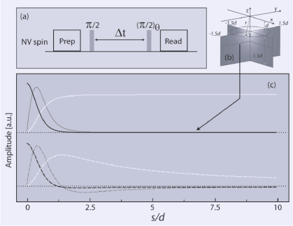
Figure 1: (a) Basic diamond-based magnetometry pulse sequence. (b) With the NV center at the reference frame origin, the grayscale indicates the relative contribution to field fluctuations from spins in a uniformly dense film. (c) In units of the relative radial coordinate $s/d$, the upper set of curves shows a cross section of the graph in (b) (black curve) and the corresponding integral (white curve). The grey curve shows the effective spin noise ‘density’ $b_{N}\left(s,z\right)$ (see text). For comparison, the lower set shows the same curves but for the average field at the NV center. Note that the integral (dashed white curve) decays slowly to zero as a result of negative contributions from spins far from the center.

Before considering the constraints deriving from the quantum character of the sensor, we describe the magnetic field generated by the nuclear spin ensemble. In an experimental setup where the NV center scans an infinitely-extended sample film, the electronic sensor spin and the nuclear spins are coupled via long-range dipolar interactions. Given that in the rotating frame resonant with the sensor spin only components of the nuclear field parallel to the $z-$axis need be taken into consideration, we find

$$\vec{{\bf B}}_{N}=B_{N}\hat{z}=\sum_{i}\left\{f\left(\vec{r}_{i}\right)\,\vec{m}_{z}^{\left(i\right)}+g\left(\vec{r}_{i}\right)\,\left(\vec{m}_{\bot}^{\left(i\right)}\cdot\hat{r}_{i}\right)\hat{z}\right\}.$$ (4)

Here $f\left(\vec{r}\right)=\left(\mu_{0}/4\pi r^{3}\right)\left(3\cos^{2}\vartheta-1\right)$ and $g\left(\vec{r}\right)=\left(3\mu_{0}/4\pi r^{3}\right)\cos\vartheta$ are functions of the distance $r_{i}=\left|\vec{r}_{i}\right|$ of the $i$-th nuclear spin to the NV center and $\vartheta_{i}$ is the angle between the position vector and the $z-$axis; $\mu_{0}$ is the magnetic permeability of vacuum, and $\vec{m}_{z}^{\left(i\right)}$ ($\vec{m}_{\bot}^{\left(i\right)}$) denotes the component of the corresponding nuclear magneton $\vec{m}^{\left(i\right)}$ parallel (perpendicular) to the $z$-axis. We will consider the situation where the distance $d$ between the sensor and the surface is of order $\sim 10$ nm or greater. We also assume that nuclear spins are dense (i.e., no nuclear spin can be singled out). In this regime, the NV center interacts with a large number of protons –exceeding $10^{5}$ in most organic samples– and thus exerts a negligible back-action on the sample system. Each nuclear spin can be described classically via a stochastic, ergodic variable featuring first and second moments $\left\langle\vec{m}\right\rangle$ and $\left\langle\vec{m}^{2}\right\rangle$, respectively.

To see that detection of the time-dependent fluctuations of the nuclear field—rather than the field itself—better suits our purpose, let us consider the case of a uniformly magnetized film and assume, for simplicity, that the normal to the sample surface coincides with the $z$-axis. Using (4) we write the time-averaged field acting on the sensor as

$$\left\langle B_{N}\right\rangle=\frac{1}{V_{p}}\int_{Film}\left\{f\left(\vec{r}\right)\,\left\langle m_{z}\right\rangle+g\left(\vec{r}\right)\,\left(\left\langle\vec{m}_{\bot}\right\rangle\cdot\hat{r}\right)\right\}\,dV,$$ (5)

where we have transformed the sums into volume integrals via the correspondence $\sum_{i}\to\;\int{\tfrac{dV}{V_{p}}}$ with $V_{p}$ representing the volume of the ‘primitive cell’ associated to a single nuclear spin. From symmetry considerations, we observe that the second term in (5) cancels out. This is also the case for the first term –in agreement with the classical magnetostatics result outside a thin, infinitely-extended, uniformly-polarized film– but here a more subtle balance between contributions from spins close and far away from the sensor is responsible Meriles05 . The latter is shown in Fig. 1c where we plot $f\left(\vec{r}\right)$ (and its integral) as a function of the (normalized) radial coordinate $s$ on the sample plane; within each thin slice of thickness $dz$, long-range, weaker contributions from more numerous spins far from the sensor exactly cancel the field created by spins contained within a central disk (of diameter comparable to the sensor-slice distance).

The concept of spin noise detection capitalizes on the spontaneous fluctuations of the nuclear spin magnetization in a small volume. To more quantitatively identify the sample volume within the film, consider the special case of a uniformly distributed, infinitely-extended sample and calculate the nuclear field variance $\Delta B_{N}^{2}$. Starting from Eq. (4) and in the limit of (5) we find

$$\Delta B_{N}^{2}=\left\langle B_{N}^{2}\right\rangle\cong\frac{1}{V_{p}}\int_{Film}\left\{\left(f\left(\vec{r}\right)\right)^{2}\left\langle m_{z}^{2}\right\rangle+\left(g\left(\vec{r}\right)\sin\vartheta\right)^{2}\left\langle m_{\bot}^{2}\right\rangle\right\}\,dV,$$ (6)

where we assumed $\left\langle m_{x}^{2}\right\rangle=\left\langle m_{y}^{2}\right\rangle=\left\langle m_{\bot}^{2}\right\rangle$. Using cylindrical coordinates for convenience, we plot in Fig. 1c the ‘spin noise density’, $b_{N}(s,z)\,ds\,dz=\frac{1}{V_{p}}\int_{0}^{2\pi}\left\{\left[\left(f(s,z)\right)^{2}\langle m_{z}^{2}\rangle+\left(g(s,z)s/\sqrt{z^{2}+s^{2}}\right)^{2}\langle m_{\bot}^{2}\rangle\right]\,s\,d\varphi\right\}\,\,ds\,dz$. While spins far from the sensor have a non-negligible contribution, fluctuations of the nuclear field at the NV center are dominated by spins approximately contained within half a sphere of radius comparable to the sensor-surface distance $d$. Comparing with the prior results, we conclude that fluctuations selectively highlight spins close to the sensor –as opposed to ‘distant’ spins– not because the resulting average field is stronger but because, being less numerous, the relative field variance is larger.

A practical upper limit for the NV center-sample distance $d$ stems from the fact that the amplitude of the field fluctuations decreases sharply with the sensor-sample distance: Assuming a sample with spin density $\rho_{N}\sim 1/V_{p}$, we find

$$\Delta B_{N}\sim C\mu_{0}m_{N}\rho_{N}^{1/2}/d^{3/2},$$ (7)

with $C$ a constant of order $\sim 1/20$ obtained from integration of Eq. (6) and $m_{N}$the nuclear magneton. For example, in the case of an organic system with proton density $\rho_{N}\sim 5\times 10^{28}m^{-3}$ and assuming $d\sim 200$ nm, we obtain $\Delta B_{N}\sim 2.5$ nT, a value approaching the sensitivity limit of a room-temperature, diamond-based magnetometer Taylor08 ; Maze08 .

We note that detection of the average magnetization within the ‘active’ volume –as opposed to magnetization fluctuations –is conceivable if the contribution to the total field from spins outside this volume has been canceled. Meriles05 In this case the nuclear field $\tilde{B}_{N}$ at the NV center site has the approximate value

$$\tilde{B}_{N}\sim D\mu_{0}m_{N}\rho_{N}P,$$ (8)

independent of the sensor-surface distance. Here $P=m_{N}B_{A}/(2k_{B}T)$ is the nuclear Boltzmann polarization at temperature $T$ and $D$ is a constant of value $\sim 1/6$. Comparing Eq. (7) and (8) we find the criterion for spin noise dominance, $d\leq\left({k_{B}T/\left(m_{N}B_{A}\right)}\right)^{{2/3}}\rho_{N}^{-{1/3}}$. For example, if we take as a reference the case in which the protonated sample ($\rho_{N}\sim 5\times 10^{28}m^{-3}$) has been polarized to the equivalent of a magnetic field $B_{A}$=10 T at room temperature, we have $d\leq$500 nm.

III Sensitivity limits

Having identified the source and magnitude of the field fluctuations at the sensor site, we now turn our attention to the general problem of using a quantum object—the NV center—to gather information on the fluctuating ensemble of sample spins. The average fluorescence in the presence of the nuclear field is calculated from. Combining Eqs. (2) and (3),

$$\left\langle Tr\left\{M\rho\right\}\right\rangle=\frac{1}{2}\alpha\left(1+\cos\theta\,\left\langle\cos\phi\right\rangle\right)+\frac{1}{2}\beta\left(1-\cos\theta\,\left\langle\cos\phi\right\rangle\right),$$ (9)

where brackets indicate expectation value and average over the different configurations of the nuclear system. In Eq. (9) we assume that the nuclear magnetization is negligible and that $BN$(and therefore $\phi$) has a symmetric distribution (i.e., $\left\langle\phi^{2k+1}\right\rangle=0$, $k$=1,2,3…). By comparison with the case in which no nuclear field is present and in the limit $\left\langle\phi^{2}\right\rangle<1$, we define the signal $S_{A}$ as

$$\begin{array}[]{l}{S_{A}\equiv\left\langle Tr\left\{M\rho\right\}\right\rangle_{\phi}-\left\langle Tr\left\{M\rho\right\}\right\rangle_{\phi=0}}\\ {\quad\,\,=\left(\alpha-\beta\right)\cos\theta\frac{\left(\left\langle\cos\phi\right\rangle-1\right)}{2}e^{-\left({\Delta t/T_{2e}}\right)^{\gamma}}\approx\frac{\left\langle\phi^{2}\right\rangle}{4}\left(\beta-\alpha\right)\cos\theta\,e^{-\left({\Delta t/T_{2e}}\right)^{\gamma}}}\end{array}.$$ (10)

In deriving Eq. (10) we introduced the coherence decay of the sensor spin characterized by the relaxation time $T_{2e}$ and the exponent Dutt07 ; Childress06 $\gamma\sim 3$. Note that the presence of the nuclear field translates into a change of the NV center average fluorescence proportional to the nuclear-spin-induced phase variance. The ‘signal’ amplitude also grows linearly with the difference between the average fluorescence in each of the two possible spin states and reaches a maximum value when the phase difference $\theta$ between the excitation and projection pulses is either zero or a multiple of $\pi$ (see Fig. 1).

In order to determine the limiting signal-to-noise ratio, we make use of the property $M^{k}=a^{k}{\left|0\right\rangle}{\left\langle 0\right|}+b^{k}{\left|1\right\rangle}{\left\langle 1\right|}$ and that $\Delta a^{2}(\Delta b^{2})=\alpha(\beta)$ for Poisson variables, to calculate the variance

$$\begin{array}[]{l}{\Delta M^{2}=\left\langle Tr\left\{M^{2}\rho\right\}\right\rangle-\left\langle Tr\left\{M\rho\right\}\right\rangle^{2}=}\\ {\quad\;=\frac{1}{2}\left(\alpha+\beta\right)+\frac{1}{2}\left(\alpha-\beta\right)\cos\theta\,\left\langle\cos\phi\right\rangle e^{-\left(\Delta{t/T_{2e}}\right)^{\gamma}}+\frac{1}{4}\left(\alpha-\beta\right)^{2}\left(1-\cos^{2}\theta\,\left\langle\cos\phi\right\rangle^{2}e^{-\left(\Delta{t/T_{2e}}\right)^{\gamma}}\right)\;.}\end{array}$$ (11)

The signal-to-noise ratio, $SNR$=$S_{A}/\Delta M$ is then

$$\begin{array}[]{l}SNR^{-2}=\frac{\Delta M^{2}}{S_{A}^{2}}=\\ =\frac{8e^{2\left(\Delta t/T_{2e}\right)^{\gamma}}}{\left\langle\phi^{2}\right\rangle^{2}}\left\{\frac{\left(\alpha+\beta\right)+\left(\alpha-\beta\right)\cos\theta\,e^{-\left(\Delta t/T_{2e}\right)^{\gamma}}}{\left(\alpha-\beta\right)^{2}\cos^{2}\theta}\right\}+\frac{4e^{2\left(\Delta t/T_{2e}\right)^{\gamma}}}{\left\langle\phi^{2}\right\rangle^{2}}\left\{\frac{1-\cos^{2}\theta\left(1-\left\langle\phi^{2}\right\rangle\right)e^{-\left(\Delta t/T_{2e}\right)^{\gamma}}}{\cos^{2}\theta}\right\}\end{array}$$ (12)

where, for simplicity, we have assumed $\left\langle\phi^{2}\right\rangle<1$ and $\cos^{2}\theta\neq 0$. Note that in the limit $e^{-\left(\Delta{t/T_{2e}}\right)^{\gamma}}\sim 1$ the first (otherwise dominant) term can be cancelled if we choose $\theta=\pi$ and assume that ${\left|m_{s}=1\right\rangle}$ is a ‘dark’ state (i.e., $\beta=0$). The latter, however, is not always the case in practice because, as pointed above, we have $\alpha\cong 1.5\beta$ for direct NV spin detection. Therefore, we recast (12) in the approximate form

$$SNR\approx 0.1\,\left\langle\phi^{2}\right\rangle\sqrt{\alpha}\,e^{-\left(\Delta{t/T_{2e}}\right)^{\gamma}},$$ (13)

where we made use of the fact that in current experimental settings $\alpha\cong 1.5\times 10^{-2}\ll 1$. Dutt07 ; Childress06 Hence, the optimal sensing time becomes a compromise between the increase in $SNR$ due to larger phase change $\sqrt{\left\langle\phi^{2}\right\rangle}$ and the exponential decay due to decoherence. A similar sensitivity limit is obtained from the measurement of the signal fluctuation, as explained in Appendix A.

Starting from (13), we can obtain a numerical estimate of the total time $T$ necessary for $SNR=10$: At a distance $d\sim 15$ nm from the surface, and for a densely protonated sample we use (7) to find $\Delta B_{N}\sim 110$ nT. For a sensing interval $\Delta t\sim 40\mu$s $\ll T_{2e}\sim 1$ ms we get $\left\langle\phi^{2}\right\rangle\cong 0.6$, thus requiring $NA\sim 2\times 10^{6}$ repetitions and a total time $T_{p}\cong N_{A}\Delta t\cong 60\;s$ (note that in the present case $t_{prep},t_{read}\ll\Delta t$, see Fig. 1). This sensitivity limit could be improved enormously if single-shot read out was available. Some strategies toward single-shot readout have recently been proposed, such as better collection efficiency via coupling of NV center to a nano-photonic wave-guide Babinec10 or readout enhanced by a nuclear spin memory. Jiang09 ; Neumann10 In this last strategy, nearby nuclear spins (such as the nitrogen associated with the NV center or a ¹³C) are used to store the information regarding the state of the electronic NV spin, so that a given measurement can be repeated many times by mapping back the state of nuclear spin onto the electronic spin after each readout. With this technique, it is possible to further improve the $SNR$ although at the expense of a much longer readout time (approaching several milliseconds).

IV Measurement of nuclear spin time correlations

In the previous section, we implicitly assume that the nuclear correlation time $T_{2n}$ is smaller than the single measurement time (in practice, of order $\sim\Delta t$) since successive measurements must be independent if they are to improve the $SNR$. However, the opposite regime $T_{2n}\gg\Delta t$ allows one to extract valuable spectroscopic information on the sample system. Intuitively, this is possible because, as nuclei evolve coherently from a random initial state, the correlation function—and thus the power spectrum—of sample spins can be determined from the statistics of successive, time-delayed measurements. Davenport70 Consistent with the assumption that the nuclear system evolves unperturbed by the NV center and that it behaves as a classical magnetic field, we define the autocorrelation function

$$K_{M}\left(\tau\right)=\left\langle Tr\left\{M\rho\left(\Delta t+\tau\right)\right\}\;Tr\left\{M\rho\left(\Delta t\right)\right\}\right\rangle,$$ (14)

with $\rho\left(t+\Delta t\right)$ denoting the density matrix that evolved under the action of the nuclear field between the times $t$ and $t+\Delta t$ (thus acquiring the phase $\phi(t+\Delta t)=\int_{t}^{t+\Delta t}\gamma_{e}B_{N}\left(t^{\prime}\right)dt^{\prime}$). Note that since the phase acquisition takes a time $\Delta t$, me must restrict $\tau$ in Eq. (14) and thereafter to $\tau\geq\Delta t$. Combining Eqs. (14) and (2) we find

$$K_{M}\left(\tau\right)=\frac{1}{4}\left(\alpha+\beta\right)^{2}+\frac{1}{4}\left(\alpha-\beta\right)^{2}\left(K_{c}\left(\tau\right)\cos^{2}\theta+K_{s}\left(\tau\right)\sin^{2}\theta+2\cos\theta\left\langle\cos\phi\right\rangle\right),$$ (15)

where $K_{c}\left(\tau\right)\equiv\left\langle\cos\phi\left(\tau+\Delta t\right)\;\cos\phi\left(\Delta t\right)\right\rangle$ and $K_{s}\left(\tau\right)\equiv\left\langle\sin\phi\left(\tau+\Delta t\right)\;\sin\phi\left(\Delta t\right)\right\rangle$. Using $\phi<1$, and choosing $\theta={\left(2k+1\right)\pi/2}$, we recast Eq. (14) in the simpler form

$$K_{M}\left(\tau\right)\cong\frac{1}{4}\left(\alpha+\beta\right)^{2}+\frac{1}{4}\left(\alpha-\beta\right)^{2}\left\langle\phi\left(\tau+\Delta t\right)\phi\left(\Delta t\right)\right\rangle.$$ (16)

Eqs. (16) and (10) can be used to reconstruct the autocorrelation function $K_{\phi}\left(\tau\right)\equiv\left\langle\phi\left(\tau+\Delta t\right)\,\phi\left(\Delta t\right)\right\rangle$ and to determine the sample power spectral density of the phase $f$—here having the role of a stochastic variable describing a stationary random process—via the Wiener-Khintchine theorem Davenport70

$$F_{\phi}\left(\nu\right)=\int_{-\infty}^{\infty}K_{\phi}\left(\tau\right)\,e^{-i2\pi\nu\tau}d\tau.$$ (17)

Note that because of the finite phase acquisition time, Eq. (17) is restricted to a bandwidth defined by the inverse of the separation between two successive measurements $\sim 1/\Delta t$ (and has a central observation frequency determined by $n$/$\Delta t$, with $n$ representing the number of $\pi$-pulses within the contact time $\Delta t$).

V Imaging and spectroscopy of nuclear spins in biological systems

In this section we consider examples that illustrate some of the potential advantages—and limitations—of using the proposed technique to reconstruct an image or a local nuclear spin spectrum. In each of the simulations that follow we use a virtual ‘sample spin source’ that we recreate in the most realistic way possible from results obtained with other techniques. For image reconstruction purposes we assume that the sensor—in the form of a cantilever-mounted scanning NV center—can be positioned relative to the sample surface with nanoscale precision.

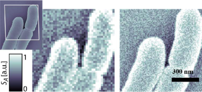
Figure 2: (Upper left insert) High-resolution SEM image of fixated E. Coli. Brighter (darker) regions correlate with high (low) spin density. (Main images) ‘Raster scan’ reconstructions of the corresponding 2D spin lattice. The color code gauges the average NV center fluorescence as determined after $NA$ observations during which the spin alignment changes randomly (see Eq. (10)). The darker regions between and on the surface of the bacteria are artifacts resulting from artificial shadowing of the source SEM image. The tip-NV center distance and raster scan resolution is 30 nm (left) and 15 nm (right). The scale bar corresponds to 300 nm. Other parameters as listed in the text.

We start by considering the SEM image of Escherichia coli shown in the insert to Fig. 2. Specimens of this kind are usually fixated in a dry environment to preserve its morphology meaning that the color code in the image correlates with the spin density of protons. The two main images in Fig. 2 show the result of our simulations for which we considered the sample as a collection of classical, independent magnetic dipoles with a short correlation time (see below). A grey scale is used to indicate the average fluorescence of the NV center at each position ($S_{A}$ in Eq. 10). In our calculations, spins were distributed on a regular lattice with 1 nm separation and were given amplitude proportional to the local proton density (as implied by the SEM source image). The NV center distance to the sample surface was kept at $d=$15 nm in one case (right) and 30 nm in the other (left). The evolution time $\Delta t$ was $40$ and $120\mu$s respectively and the number of measurements per image point was $N_{A}=4\times 10^{5}$. The resulting time per pixel $T_{p}$ is 15 s (or 50 s) and the image time $T_{i}$ is estimated at 5 hs (or 4 hs) for a square of (500 nm)². We note that longer exposure times will be necessary if other, non-fundamental sources of noise are present; this scenario, however, is unlikely in an optimized confocal microscope where operation has been shown to be photon shot-noise limited. Maze08

One aspect of our example that deserves special consideration concerns the values assumed for the nuclear correlation and electron coherence times. First, we note that after fixation the system of Fig. 2 can be considered a solid with the result that the nuclear correlation time $T_{N}$ –assuming an external field $B_{A}$ stronger than the internuclear dipolar interaction– is dictated by $T_{1N}$, the nuclear spin-lattice relaxation time. Because under realistic conditions $T_{1N}$ largely exceeds $\Delta t$, the time required for a raster scan of the sample grows to impractical values if the nuclear spin configuration at a given position must change randomly before the next measurement is carried out. Fortunately, there are ways to circumvent this problem, the simplest being to probe other points of the sample surface during the wait time.

Attaining the longest coherence time in a NV center –exceeding 1 ms in isotopically depleted samples Balasubramanian09 – demands intercalating a $\pi$-pulse at the midpoint of the evolution time $\Delta t$. Dutt07 ; Childress06 While, for simplicity, our calculations have obviated this need , one immediate practical consequence is that a synchronous $\pi$-rotation must be applied on the sample spins if the net effect of the sample dipolar field on the sensor is to be preserved. In the presence of an auxiliary dc field $B_{A}\sim 200$ gauss, the latter can be carried out via a resonant ‘radio-frequency’ pulse (at $\sim 1$ MHz).

Although spin density mapping is the most basic form of imaging, it is ultimately the ability to introduce contrast between different soft tissues that separates MRI from other imaging technologies. Some of the contrast methodologies used in MRI find a natural extension in our detection strategy. For example, molecular diffusion away from the immediate vicinity of the sensor results in a shortening of the nuclear correlation time, which, with a suitable selection of $\Delta t$, can be exploited to make the time-averaged phase shift $\phi$ negligibly small.The latter is shown in Fig. 3 where we used an SEM image from the membrane of a red blood cell to encode the correlation time of spins on a uniformly dense lattice (i.e., spins in the void spaces of the SEM image were assigned a shorter nuclear correlation time). This example provides a rudimentary model for a ‘water-filled’ membrane whose semi-rigid skeleton can be distinguished from the embedded fluid.

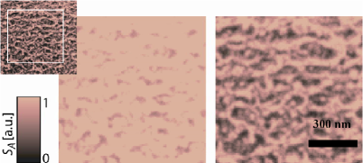
Figure 3: (Insert) SEM image of the membrane of a red blood cell. Void spaces become apparent only after dehydration and fixation. (Main images) Unlike Fig. 2, the virtual 2D spin matrix is uniform (emulating the case of a ‘wet membrane’). This time the color scale of the source image was used to encode the local nuclear spin correlation time. In the example presented on the left, ‘mobile’ regions (corresponding to dark regions in the source image) have a correlation time only 1.3 times shorter than the rest. The image on the right is based upon identical conditions except that the correlation time difference was three times greater. The scale bar corresponds to 300 nm.

In situations similar to that of Fig. 3, Eq. (17) could be used, for example, to monitor diffusion processes. In this context, we note that one of the most important structural characteristics of the cell membrane is that it behaves like a two-dimensional liquid, i.e., its constituent molecules rapidly move about in the membrane plane. Therefore, one could imagine extensions of the basic pulse protocol to emulate their corresponding NMR counterparts (but with resolution on the tens of nanometers). In principle, a broad range of diffusion rates is within reach (because the probing time can be greatly enhanced if, after a given evolution period, the NV center coherence is stored in an adjacent ¹³C nucleus for future retrieval Dutt07 ). Studies of this kind may prove worthy, especially if we keep in mind that although the structure of plasma membranes is known to be inhomogeneous, the precise architecture of this important system still remains unclear. Lillemeier06

In a different implementation where the auxiliary field $B_{A}$ points along an axis non-collinear with the crystal field one could rely on the above formalism to extract spectroscopic information from random nuclear spin coherences. An example is shown in Fig. 4 where we consider a set of (model) molecules with a 13 Hz heteronuclear (e.g., proton-phosphorous) $J-$coupling. In our simulation the auxiliary magnetic field $B_{A}$ is 20 gauss, the tip distance is 30 nm, and the system correlation time is 100 ms. Assuming the sensor at a fixed position in space, Fig. 4 shows the pulse sequence and resulting autocorrelation function and power spectral density. Implicit in this model is the idea that molecules tumble and move relative to each other so as to cancel inter- and intramolecular dipolar couplings without escaping the observation volume of the sensor during $\Delta t$. Our example mimics the conditions of ‘restricted diffusion’ found, for example, within a cell membrane where molecules ‘hop’ between adjacent, $\sim(100nm)^{3}$ compartments on a time scale of several milliseconds. Murase04

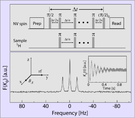
Figure 4: In this example the NV center repeatedly monitors a set of equivalent protons subject to a 6.5 Hz heteronuclear $J$-coupling with a second (invisible) spin-1/2 species. Depending on the alignment of the latter, protons precess with one of two possible frequencies. (Top) Schematics of the pulse sequence; $n$ denotes the number of p-pulses within the evolution interval $\Delta t$. (Bottom) Reconstructed correlation (insert) and corresponding spectral density. Note the factor 2 in the observed splitting (13 Hz), a direct consequence of having assumed $\left|\cos\theta\right|=1$ (‘quadratic response’). In the simulation $n$=1, $d=$30 nm and $\Delta t$=100 ms. The nuclear correlation time is 100 ms, and the number of single measurement pairs per point in the correlation curve is 4x105. The external magnetic field $B_{A}$is 5 mT and pulses acting on nuclear spins are assumed to be broadband so as to invert proton spins as well as the $J$-coupled species. Other conditions as listed in the text.

VI Conclusion

While high-field MRI serves as a superb tool to probe the living world, achieving submicroscopic spatial resolution presently appears to be a goal exceedingly difficult. Indirect detection via NV centers in diamond provides an alternative platform that we examined by means of analytical and numerical calculations. We considered the particular case of a single NV center interacting with a large number of nuclear spins, a condition that we described in semiclassical terms. When brought in close proximity to the sample surface, e.g. with the aid of a high-precision scanner, the NV center is selectively sensitive to field fluctuations induced by nuclear spins immediately adjacent to the sensor (even if the mean sample magnetization is negligible). The important practical consequence is that pre-polarization magnet, gradient coils, and fast-switching current amplifiers—today mandatory in a nuclear spin imaging experiment—are not requisites of this technology.

Our calculations show that simple Ramsey or spin-echo sequences are able to probe the nuclear spin system although the relative phase between pulses plays a crucial role. Under current experimental conditions, photon shot noise is the main source of error. We stress, however, that the sources of this limitation are not fundamental and that technical advances could lead to significant decrease in the imaging times.

When compared to other kinds of microscopies, several distinguishing features of NV center-based magnetometry emerge. For example, given the sharp dependence on the sensor-sample distance, detection is restricted to surface spins (with the result that careful sample preparation will be necessary when inner structures of a system are to be exposed). On the other hand, the same setup could be exploited to reconstruct 3D topographic maps that can then be used to enrich the information content of the images produced via the NV center fluorescence. Even if exposure times longer than those typical of other imaging schemes are necessary, diamond-based magnetometry has the potential to gauge changes in the dynamics and chemical composition of the sample, thus opening the door to various types of contrast. In particular, we have shown that, with an adequate protocol, one could probe molecular diffusion or reconstruct the low- or zero-field nuclear spin spectrum McDermott02 ; Weitekamp83 with nanoscale spatial resolution. Finally, we note that most biochemical reactions are thermally-driven, stochastic processes that involve the crossing of a barrier or diffusion over some kind of potential energy surface. Therefore, the ability to conduct experiments in an open environment, at room temperatures can prove crucial to expose the dynamics of living systems in ways not possible with traditional magnetic resonance. For example, with spatial resolution of $\sim 5$ nm—only slightly better than our target here—one could envision investigating the stepping of single molecular motors, a process that usually takes place in the tens of milliseconds range.

Appendix A

While through Eq. (10) we monitor sample spins via changes in the average number of photons emitted by the sensor, similar information can be obtained if we measure instead changes in the fluorescence variance. This strategy closely mimics that already demonstrated in magnetic force microscopy7 and, within the framework presented above, appears as a ‘natural’ alternate pathway. Starting from (11) and neglecting for simplicity relaxation, a simple calculation shows that the signal $S_{V}$ in this case is given by

$$S_{V}\equiv\Delta M_{\phi}^{2}-\Delta M_{\phi=0}^{2}\cong\frac{1}{4}\cos\theta\,\left(\alpha-\beta\right)\left(\left(\alpha-\beta\right)\cos\theta-1\right)\left\langle\phi^{2}\right\rangle.$$ (18)

To determine the limit uncertainty, we define the auxiliary operator $V\equiv\left(M-\left\langle Tr\left\{M\rho\right\}\right\rangle\right)^{2}$ and calculate $\Delta V^{2}=\left\langle Tr\left\{\left(V-\left\langle Tr\left\{V\rho\right\}\right\rangle\right)^{2}\rho\right\}\right\rangle$. In the limit in which the shot noise is stronger than the spin noise, we find after a lengthy but straightforward calculation $\Delta V^{2}\cong\alpha$. Therefore, the signal to noise ratio is given in this case by

$$SNR=\frac{S_{V}}{\Delta V}\cong 0.1\,\left\langle\phi^{2}\right\rangle\sqrt{\alpha},$$ (19)

in agreement with (13).

We note that $S_{A}$ in Eq. (10) –and thus $S_{V}$, Eq. (18)– is insensitive to fluctuations of the nuclear field if the phase difference $\theta$ between the excitation and projection pulses is an odd multiple of $\pi/2$. In a way, this condition is counterintuitive because, in a sequence where the pulses are phase-shifted, the magnetometer responds linearly—not quadratically—to external fluctuations prompting the question as to whether higher sensitivity can be reached.

Though in a different context, Wineland and collaborators have discussed similar problems extensively. Itano93 Their work highlights the ambiguity that stems from the quantum character of the sensor via the concept of ‘quantum projection noise’: When a single two-level system probes a (non-fluctuating) magnetic field, maximum sensitivity comes at the price of complete uncertainty in the outcome of a measurement; reciprocally, when the measurement variance is zero, so is the sensitivity to external fields. Although in the present case the ‘signal’ comes in the form of fluctuations of the magnetometer phase, this principle does play here an important (if more subtle) role. We can make it explicit by rewriting (11) as

$$\Delta M^{2}=\Delta M_{q}^{2}+\Delta M_{c}^{2},$$ (20)

where $\Delta M_{q}^{2}=\left\langle Tr\left\{M^{2}\rho\right\}-\left(Tr\left\{M\rho\right\}\right)^{2}\right\rangle$ and $\Delta M_{c}^{2}=\left\langle\left(Tr\left\{M\rho\right\}\right)^{2}\right\rangle-\left\langle Tr\left\{M\rho\right\}\right\rangle^{2}$. The first contribution measures the ‘quantum projection noise’ or uncertainty in a population measurement of a single two level system; the second term corresponds to the nuclear-spin-noise-induced variance in a ‘classical’, macroscopic-like sensor (where the average polarization can be determined from a single measurement). If, for simplicity, we consider in Eq. (2) $a=1$ and $b=0$, we find after a simple calculation

$$\Delta M_{q}^{2}=\frac{1}{4}\left(1-\left\langle\cos^{2}\left(\phi+\theta\right)\right\rangle\right),$$ (21)

and

$$\Delta M_{c}^{2}=\frac{1}{4}\left(\left\langle\cos^{2}\left(\phi+\theta\right)\right\rangle-\left\langle\cos\left(\phi+\theta\right)\right\rangle^{2}\right).$$ (22)

For the special case $\theta=(2k+1)\pi/2$ it follows $\Delta M_{c}^{2}=\frac{1}{4}\left\langle\sin^{2}\phi\right\rangle$ and $\Delta M_{q}^{2}=\frac{1}{4}\left(1-\left\langle\sin^{2}\phi\right\rangle\right)$ meaning that as we increase the amplitude of the external field fluctuations, the gain in the ‘classical’ contribution to the variance is lost because of an equal but opposite change of the quantum projection noise. This is no longer the case when $\theta=k\pi$ thus leading to an observable change in the variance of the sensor fluorescence.

References

- (1) J.M. Taylor, P. Cappellaro, L. Childress, L. Jiang, D. Budker, P.R. Hemmer, A. Yacoby, R. Walsworth, M.D. Lukin, High-sensitivity diamond magnetometer with nanoscale resolution, Nature Phys. 4, 810 (2008).
- (2) C.L. Degen, Scanning magnetic field microscope with a diamond single spin sensor, App. Phys. Lett 92, 243111 (2008).
- (3) D. Budker, M. Romalis, Optical magnetometry, Nat. Phys. 3, 227 (2007).
- (4) G. Balasubramanian, P. Neumann, D. Twitchen, M. Markham, R. Kolesov, N. Mizuochi, J. Isoya, J. Achard, J. Beck, J. Tissler, V. Jacques, P.R. Hemmer, F. Jelezko, J. Wrachtrup, Ultralong spin coherence time in isotopically engineered diamond, Nat. Mat. 8, 383 (2009).
- (5) J.R. Maze, P.L. Stanwix, J.S. Hodges, S. Hong, J.M. Taylor, P. Cappellaro, L. Jiang, M.V. Gurudev Dutt, E. Togan, A.S. Zibrov, A. Yacoby, R.L. Walsworth, M.D. Lukin, Nanoscale magnetic sensing with an individual electronic spin in diamond , Nature 455, 644 (2008).
- (6) G. Balasubramanian, I.Y. Chan, R. Kolesov, M. Al-Hmoud, J. Tisler, C. Shin, C. Kim, A. Wojcik, P.R. Hemmer, A. Krueger, T. Hanke, A. Leitenstorfer, R. Bratschitsch, F. Jelezko, J. Wrachtrup, Nanoscale imaging magnetometry with diamond spins under ambient conditions, Nature 455, 648 (2008).
- (7) C.L. Degen, M. Poggio, H.J. Mamin, D. Rugar, Role of spin noise in the detection of nanoscale ensembles of nuclear spins”, Phys. Rev. Lett. 99, 250601 (2007).
- (8) C.A. Meriles, Optical detection of nuclear magnetic resonance at the sub-micron scale, J. Magn. Reson. 176, 207 (2005).
- (9) M.V. Gurudev Dutt, L. Childress, L. Jiang, E. Togan, J. Maze, F. Jelezko, A.S. Zibrov, P.R. Hemmer, M.D. Lukin, Quantum register based on individual electronic and nuclear spin qubits in diamond, Science 316, 1312 (2007).
- (10) L. Childress, M.V. Gurudev Dutt, J.M. Taylor, A.S. Zibrov, F. Jelezko, J. Wrachtrup, P.R. Hemmer, M.D. Lukin, “Coherent dynamics of coupled electron and nuclear spin qubits in diamond”, Science 314: 281 (2006).
- (11) T. Babinec, B.J.M. Hausmann, M. Khan, Y. Zhang, J. Maze, P.R. Hemmer, M. Loncar, A diamond nanowire single-photon source, Nat. Nanotechnol. 5, 195 (2010).
- (12) L. Jiang, J.S. Hodges, J.R. Maze, P. Maurer, J.M. Taylor, D.G. Cory, P.R. Hemmer, R.L. Walsworth, A. Yacoby, A.S. Zibrov, M.D. Lukin, M. D., Repetitive Readout of a Single Electronic Spin via Quantum Logic with Nuclear Spin Ancillae, Science 326, 267 (2009).
- (13) Neumann et al., private communication.
- (14) W.B. Davenport (1970), Probability and Random Processes, New York, McGraw-Hill.
- (15) B.F. Lillemeier, J.R. Pfeiffer, Z. Surviladze, B.S. Wilson, M.M. Davis, Plasma membrane-associated proteins are clustered into islands attached to the cytoskeloton, Proc. Natl. Acad. Sci USA 103, 18992 (2006).
- (16) K. Murase, T. Fujiwara, Y. Umemura, K. Suzuki, R. Iino, H. Yamashita, M. Saito, H. Murakoshi, K. Ritchie, A. Kusumi, Ultrafine membrane compartments for molecular diffusion as revealed by single molecule techniques, Biophys. J. 86, 4075 (2004).
- (17) R. McDermott, A.H. Trabesinger, M. M ck, E.L. Hahn, A. Pines, J. Clarke Liquid-State NMR and Scalar Couplings in Microtesla Magnetic Fields, Science 295, 2247 (2002).
- (18) D.P. Weitekamp, A. Bielecki, D. Zax, K. Zilm, A. Pines, Zero-field nuclear magnetic resonance, Phys. Rev. Lett. 50, 1807 (1983).
- (19) W.M. Itano, J.C. Bergquist, J.J. Bollinger, J.M. Gilligan, D.J. Heizen, F.L. Moore, M.G. Raizen, D.J. Wineland, Quantum projection noise: Population fluctuations in two-level systems, Phys. Rev. A 47, 3554 (1993).