Localization and Fractality in Inhomogeneous Quantum Walks with Self-Duality

Abstract

We introduce and study a class of discrete-time quantum walks on a one-dimensional lattice. In contrast to the standard homogeneous quantum walks, coin operators are inhomogeneous and depend on their positions in this class of models. The models are shown to be self-dual with respect to the Fourier transform, which is analogous to the Aubry-André model describing the one-dimensional tight-binding model with a quasi-periodic potential. When the period of coin operators is incommensurate to the lattice spacing, we rigorously show that the limit distribution of the quantum walk is localized at the origin. We also numerically study the eigenvalues of the one-step time evolution operator and find the Hofstadter butterfly spectrum which indicates the fractal nature of this class of quantum walks.

I Introduction

A quantum walk (QW) Gudder ; Aharonov ; Meyer , the quantum mechanical analogue of the classical random walk (RW), is a useful tool to promote various fields. For instance, the QW is an important primitive in universal quantum computation Childs ; Lovett and efficient quantum algorithms Shenvi ; Ambainis2 ; Buhrman ; Magniez ; Magniez2 . The realization of topological phases Kitagawa and quantum phase transitions Chandrashekar in optical lattice systems by the QW have been discussed. The relation between the Landau-Zener transition and the QW was found in Ref. Oka . The QW provides a new clue to more fundamental problems such as the quantum foundations of time Shikano and the photosynthesis and efficient energy transfer in biomolecules Engel ; Mohseni . There are several important properties of the QW: (i) the inverted-bell like limit distribution, (ii) the quadratic speed-up of the variance to the classical RW, and (iii) the localization due to the quantum coherence and interference. The physical, mathematical, and computational properties of the QW are summarized in Refs. Kempe ; KonnoRev ; Kendon ; Venegas-Andraca .

In this paper, we focus on the localization property of the QW and study a class of the discrete-time quantum walk (DTQW) on a one-dimensional lattice with spatially inhomogeneous coins. Throughout this paper, we define the localization such that the limit distribution of the DTQW divided by some power of the time variable has the probability density given by the Dirac delta function. The localization in the DTQW with homogeneous coins has so far been extensively studied. In the one dimensional DTQW, the localization was shown in the models with a three-dimensional coin Inui , a four-dimensional coin Inui2 , a two-dimensional coin with memory McGettrick , a two-dimensional coin in a random environment Joye and a time-dependent two-dimensional coin; the Fibonacci QW Romanelli . On the other hand, the nature of the localization in the two-dimensional DTQW has been studied numerically Mackay ; Tregenna and analytically Inui3 ; Watabe . The DTQW on the Cayley tree with a multi-state coin was also studied Chisaki . Furthermore, the recurrence properties of the DTQW, i.e., the decay rate of the probability at the origin, were studied in Refs. Wojcik ; Stefanak ; Stefanak2 ; Chandrashekar2 ; Xu . Recently, the localization property of the DTQW with the inhomogeneous two-dimensional coin has been analytically shown in the model in which the coin at the origin is different from the rest Konno1 ; Konno2 and in the model of the periodically inhomogeneous coins Linden . In this paper, we generalize the model investigated in Ref. Linden to the incommensurate case and show the localization property of the generalized model.

The generalized model defined in the next section is inspired by the Aubry-André model Aubry_Andre , which describes the one-dimensional tight-binding model with an incommensurate potential. The corresponding Schrödinger equation is called the almost Mathieu equation Barry_Simon :

$$\psi(n+1)+\psi(n-1)+V\cos(2\pi\alpha n)\psi(n)=E\psi(n),$$ (1)

where $\psi(n)$ is the amplitude of the wavefunction at the $n$th site, $\alpha$ is the irrational number, and $E$ is the eigenenergy. The model is often used to study the localization-delocalization transition Sokoloff . Aubry and André have shown that all the eigenstates are localized when $V>2$ while they are extended when $V<2$. The model was shown to be self-dual with respect to the Fourier transform at $V=2$ Aubry_Andre . The critical point $V=2$ is closely related to the Azbel-Hofstadter problem, which is the eigenvalue problem of the Bloch electron on a square lattice in a uniform magnetic field Azbel ; Hofstadter . The energy spectrum shows a self-similar and fractal structure known as the Hofstadter butterfly Hofstadter . The multifractal property of the spectrum and wavefunctions have been studied in Refs. Kohmoto_1983 ; Tang_Kohmoto and its Bethe ansatz solution was discussed in Refs. Wiegmann ; Hatsugai_Kohmoto_Wu ; Abanov . In this paper, we show that our QW model is self-dual under the Aubry-André duality transformation. We also study the eigenvalues of the one-step time evolution of our QW and find that the spectrum shows a self-similar and fractal structure in analogy to the Hofstadter butterfly.

The paper is organized as follows. In Sec. II, we define the DTQW with spatially inhomogeneous coins and show that this model is self-dual under a certain transformation, which is analogous to the Aubry-André duality. In Sec. III, we rigorously show that the limit distribution of our DTQW model is localized at the origin, which means that the distribution has the finite support for any time. In Sec. IV, we numerically study the eigenvalues of the unitary operator for the one-step time evolution in our model and show the spectrum as a function of the inverse period (the Hofstadter butterfly diagram). Section V is devoted to the summary and discussion.

II Inhomogeneous Quantum Walk and Aubry-André Duality

Let us define the one-dimensional DTQW Ambainis as follows. First, we prepare the position and coin states denoted as $|{n}\rangle\otimes|{\zeta}\rangle=|{n,\zeta}\rangle$. Here, the position $n$ is along the infinite one-dimensional lattice $\mathbb{Z}$ (the integers) and $|{\zeta}\rangle$ is a normalized linear combination of $|{L}\rangle=(1,0)^{{\bf T}}$ and $|{R}\rangle=(0,1)^{{\bf T}}$, where ${\bf T}$ is the transposition. Second, we describe the time evolution of the DTQW using the unitary operator $U$ defined by two kinds of unitary operations ${\hat{C}}$ and $W$. The quantum coin flip ${\hat{C}}\in U(2)$ corresponds to the coin flip at each site in the RW. By the shift operator $W$, the position $n$ changes depending on the coin state:

$$W|{n,L}\rangle :=|{n-1,L}\rangle,$$

$$W|{n,R}\rangle :=|{n+1,R}\rangle.$$ (2)

We can explicitly write the shift operator as

$$W=\sum_{n}\left(|n-1,L\rangle\langle n,L|+|n+1,R\rangle\langle n,R|\right).$$ (3)

Then, the one-step time evolution for the DTQW is expressed as $U=W(Id.\otimes\hat{C})$, where $Id.$ expresses the identity operator. Starting from the initial state $|{0,\phi}\rangle$, we apply $U$ to the state at every step. After the $t$ time steps, we obtain the probability distribution at the position $n$ as

$$\Pr(n;t)=\sum_{\xi\in\{L,R\}}\left|\langle{n,\xi}|U^{t}|{0,\phi}\rangle\right|^{2}.$$ (4)

In the following, we introduce the DTQW with the spatially inhomogeneous coins. In this class of models, the quantum coin flip at each site can be different from the others. The coin operator $C$ acting on the position and coin states is then given by

$$C= \sum_{n}\left[(\cos(2\pi\alpha n)|n,L\rangle+\sin(2\pi\alpha n)|n,R\rangle)\langle n,L|\right.$$

$$\ \,\left.+(\cos(2\pi\alpha n)|n,R\rangle-\sin(2\pi\alpha n)|n,L\rangle)\langle n,R|\right].$$ (5)

More explicitly, the operator $C$ is written in the following form

$$C =\sum_{n}\left[|{n}\rangle\langle{n}|\otimes\left(\begin{array}[]{cc}\cos(2\pi\alpha n)&-\sin(2\pi\alpha n)\\ \sin(2\pi\alpha n)&\cos(2\pi\alpha n)\end{array}\right)\right]$$ (8)

$$:=\sum_{n}\left[|{n}\rangle\langle{n}|\otimes{\hat{C}}_{n}\right],$$ (9)

where $\alpha$ is a real number ($\alpha\in\mathbb{R}$) and corresponds to the inverse period of the coin operations. This inverse period can even be incommensurate to the underlying lattice. It reminds us of the Aubry-André model Aubry_Andre . We call this model the inhomogeneous QW throughout this paper. Note that, this model is a generalization of that in Ref. Linden . As an example, in Fig. 1 we show the behavior of the probability distribution at the $1000$th step obtained by numerical iteration.

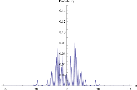
Figure 1: Probability distribution in the inhomogeneous QW after the $1000$ time steps. Here, we take the initial coin state $(|{L}\rangle+|{R}\rangle)/\sqrt{2}$ and the inverse period $\alpha=\pi/2$, which is an irrational number. Note that, the probability outside the plot range is zero within the numerical accuracy.

We shall now show that the inhomogeneous QW is always self-dual under a certain duality transformation. Let us introduce a duality transformation, which corresponds to the spatial Fourier transform Grimmett ,

$$|n,{\tilde{L}}\rangle=\sum_{m}\left[\sin(2\pi\alpha mn)|m,L\rangle+\cos(2\pi\alpha mn)|m,R\rangle\right],$$

$$|n,{\tilde{R}}\rangle=\sum_{m}\left[\cos(2\pi\alpha mn)|m,L\rangle+\sin(2\pi\alpha mn)|m,R\rangle\right].$$ (10)

It should be noted that these states are not normalized. Let us now see the action of the shift operator $W$ on these states. One can easily check the following relations

$$W|n,{\tilde{L}}\rangle=\cos(2\pi\alpha n)|n,{\tilde{L}}\rangle+\sin(2\pi\alpha n)|n,{\tilde{R}}\rangle,$$

$$W|n,{\tilde{R}}\rangle=\cos(2\pi\alpha n)|n,{\tilde{R}}\rangle-\sin(2\pi\alpha n)|n,{\tilde{L}}\rangle.$$ (11)

It is now obvious that the shift operator $W$ acts like a coin operator in the dual basis. Similarly, the action of the operator $C$ in the dual basis is given by

$$C|n,{\tilde{L}}\rangle=|n-1,{\tilde{L}}\rangle,$$

$$C|n,{\tilde{R}}\rangle=|n+1,{\tilde{R}}\rangle,$$ (12)

and it can be regarded as the shift operator in the dual basis. In this way, the duality transformation completely interchange the roles of $W$ and $C$. Therefore, the inhomogeneous QW is self-dual under the transformation (10).

III Limit Localized Distribution

In this section, we analytically show the localization in the inhomogeneous QW as the following theorem.

Theorem 1.

For any irrational $\alpha\in{\mathbb{R}}\setminus{\mathbb{Q}}$, the limit distribution of the inhomogeneous QW divided by any power of the time variable is localized at the origin:

$$\frac{X_{t}}{t^{\theta}}\Rightarrow I~{}~{}~{}~{}(t\to\infty),$$ (13)

where $X_{t}$ is the random variable for the position at the $t$ step (FG, , Ch. 2), $\theta\ (>0)$ is an arbitrary parameter, and “$\Rightarrow$” means convergence in distribution comment . Here, the limit distribution $I$ has the probability density function $f(x)=\delta(x)~{}~{}(x\in{\mathbb{R}})$, where $\delta(\cdot)$ is the Dirac delta function. Note that, the limit distribution $I$ is independent of the parameter $\theta$.

This theorem is the main result of this paper and means that the distribution of the inhomogeneous QW has a finite support for almost all $\alpha$. We first show the following lemma to prove the above theorem in the case of specific rational $\alpha$.

Lemma 1.

When $\alpha=\frac{P}{4Q}\in\mathbb{Q}$ with relatively prime $P$ (odd integer) and $Q$, the inhomogeneous QW is restricted to the finite interval $[-Q,Q]$.

Proof.

Let us express the state at the $t$ step evolving from the initial state $|{0,\phi}\rangle$ as

$$(WC)^{t}|{0,\phi}\rangle=\sum_{n\in\mathbb{Z}\atop\xi\in\{L,R\}}\psi_{t}(n;\xi)|{n,\xi}\rangle.$$ (14)

Then, we obtain the one-step time evolution of the coefficients $\psi_{t}(n;\xi)$ as follows:

$$\psi_{t+1}(n-1;L)$$

$$\ \ =\cos(2\pi\alpha n)\psi_{t}(n;L)-\sin(2\pi\alpha n)\psi_{t}(n;R),$$

$$\psi_{t+1}(n+1;R)$$

$$\ \ =\sin(2\pi\alpha n)\psi_{t}(n;L)+\cos(2\pi\alpha n)\psi_{t}(n;R).$$ (15)

Since $\cos(\pm 2\pi\alpha mQ)=0$ for any odd integer $m$, that is, the diagonal elements of the coin operator are zero at position $\pm mQ$, we immediately arrive at

$$\psi_{t+1}(\pm mQ-1;L) =\pm(-1)^{\frac{mP+1}{2}}\psi_{t}(\pm mQ;R),$$

$$\psi_{t+1}(\pm mQ+1;R) =\mp(-1)^{\frac{mP+1}{2}}\psi_{t}(\pm mQ;L).$$ (16)

The above equations mean that the quantum walker is reflected at the position $n=\pm mQ$ and cannot be transmitted across this point (see Fig. 2). Since the initial position is localized at the origin ($n=0$), the quantum walker undergoes reflection only at the sites $\pm Q$. Therefore, we conclude that the distribution of the inhomogeneous QW has the finite support $[-Q,Q]$ for any time $t$.

Figure 2: Time evolution of the inhomogeneous QW around the site $\pm mQ$ at which the quantum walker is reflected. The coin operator $C$ and shift operator $W$ act on the wavefunction $|{\psi_{n}(t)}\rangle=(\psi_{t}(n,L),\psi_{t}(n,R))^{{\bf T}}$ at each site $n$. The wavefunction around the reflection point $\pm mQ$ is indicated from the $(t_{r}-1)$th step to the $(t_{r}+1)$th step.

∎

From Lemma 1, we can conclude that our inhomogeneous QW is finitely restricted when $\alpha=\frac{P}{4Q}\in\mathbb{Q}$. We now try to extend this result to the case of $\alpha\in{\mathbb{R}}\setminus{\mathbb{Q}}$ and show Theorem 1. The following well-known theorem in number theory is useful. The proof of this theorem can be found in Ref. Hardy .

Theorem 2 (Dirichlet’s Approximation Theorem (Hardy, , Theorem 185)).

For any irrational number $\alpha\in{\mathbb{R}}\setminus{\mathbb{Q}}$, there is an infinity of the fractions $a/b$ which satisfy

$$\left|\alpha-\frac{a}{b}\right|<\frac{1}{b^{2}}.$$ (17)

Theorem 17 implies the following corollary which will be used to prove Theorem 1.

Corollary 1.

For any irrational number $\alpha\in{\mathbb{R}}\setminus{\mathbb{Q}}$, there is an infinity of the fractions $\frac{P}{4Q}$ with the relatively prime $P$ (odd integer) and $Q$ which satisfy

$$\left|\alpha-\frac{P}{4Q}\right|<\frac{1}{4Q^{2}}.$$ (18)

Proof.

From Theorem 17, for any irrational number $\alpha^{\prime}\in{\mathbb{R}}\setminus{\mathbb{Q}}$, there is an infinity of the fractions $P^{\prime}/Q$ which satisfy

$$\left|\alpha^{\prime}-\frac{P^{\prime}}{Q}\right|<\frac{1}{Q^{2}}.$$ (19)

$P^{\prime}$ can be expressed as $P^{\prime}=P\times 2^{\ell}$ with an odd integer $P$ and a non-negative integer $\ell$. It is noted that $P$ and $Q$ are relatively prime since $P^{\prime}/Q$ is an irreducible fraction. Therefore, dividing both sides of the above equation by $2^{\ell+2}$, we obtain

$$\left|\frac{\alpha^{\prime}}{2^{\ell+2}}-\frac{P}{4Q}\right|<\frac{1}{2^{\ell+2}Q^{2}}\leq\frac{1}{4Q^{2}}.$$ (20)

Since $\alpha:=\alpha^{\prime}/2^{\ell+2}$ must be irrational, we obtain the desired result. ∎

In the following, we prove Theorem 1.

Proof of Theorem 1.

For any $\epsilon>0$, there exist the relatively prime $P$ (odd integer) and $Q>\frac{\pi}{2\epsilon}$ such that

$$\alpha=\frac{P}{4Q}+\delta,$$ (21)

where $-1/(4Q^{2})<\delta<1/(4Q^{2})$ according to Corollary 18. We calculate the diagonal elements of the coin operator at the $\pm Q$th site as

$$\cos\left[2\pi\left(\frac{P}{4Q}+\delta\right)(\pm Q)\right]=(-1)^{(P+1)/2}\sin(2\pi Q\delta).$$ (22)

Note that both the diagonal elements of ${\hat{C}}_{\pm Q}$ are equal. We obtain

$$\left|(-1)^{(P+1)/2}\sin(2\pi Q\delta)\right|<\frac{\pi}{2Q}<\epsilon.$$ (23)

Since $\epsilon$ can be arbitrarily small, the diagonal element is zero in the limit. Then, along the same lines as Lemma 1, the inhomogeneous QW is restricted to the finite interval $[-Q,Q]$. Since the time variable $t$ and the parameter $\epsilon$ are independent, the time variable $t$ and the parameter $Q$ are also independent. Therefore, we obtain the desired result (13). ∎

Analogous to the above discussion, we show the localization property of the DTQW with spatially random coins as follows. From Lemma 1, we obtain the following remark, which was implicitly shown in Ref. Linden .

Remark 1.

If the diagonal elements of the coin operator at a position on each side the origin are zero, then the DTQW is finitely restricted, i.e., the localization at the origin as in Eq. (13).

Therefore, the limit distribution of the DTQW with a randomly chosen quantum coin ${\hat{C}}_{n,{\rm random}}$ with uniform distribution in $U(2)$ at each position $n\ (\in{\mathbb{Z}})$ divided by any power of the time variable is also localized. This is because the diagonal elements of ${\hat{C}}_{n,{\rm random}}$ must be zero at some positions. This result is relevant to Ref. Joye .

IV Fractal Property

In this section, we study the eigenvalues of the operator $WC$, which is the one-step time evolution in the inhomogeneous QW and is defined in Eqs. (3, 5). We show the general properties of the eigenvalues as well as the numerically obtained distribution of them, which suggests the self-similar and fractal structure in the spectrum in analogy to the Hofstadter butterfly problem.

We first show the following theorem for the eigenvalues of the operators $WC$ and $CW$.

Theorem 3.

All the eigenvalues of the operators $WC$ and $CW$ are identical including the degeneracy.

Proof.

Let $|{\mu}\rangle$ be an eigenvector of the operator $WC$ with a nonzero eigenvalue $\mu$:

$$WC|{\mu}\rangle=\mu|{\mu}\rangle.$$ (24)

Note that, all the eigenvalues of $WC$ are nonzero and have modulus $1$ since $WC$ is a unitary operator. Multiplying $C$ from the left, one obtains

$$CW(C|{\mu}\rangle)=\mu(C|{\mu}\rangle).$$ (25)

Since $C$ is also a unitary operator, $C|{\mu}\rangle$ is a nonzero eigenvector of $CW$ with the eigenvalue $\mu$. To complete the proof, we need to repeat the same argument for $CW$. Let $|{\lambda}\rangle$ be an eigenvector of $CW$ with an eigenvalue $\lambda$:

$$CW|{\lambda}\rangle=\lambda|{\lambda}\rangle.$$ (26)

Multiplying $W$ from the left, one obtains

$$WC(W|{\lambda}\rangle)=\lambda(W|{\lambda}\rangle).$$ (27)

Since $W$ is a unitary operator, $W|{\lambda}\rangle$ is a nonzero eigenvector of $WC$ with the eigenvalue $\lambda$. The identical degeneracy of $WC$ and $CW$ follows from the fact that the unitary operator $C$ or $W$ preserves the orthogonality of the states with the same eigenvalue. ∎

Remark 2.

Theorem 3 holds not only for the inhomogeneous QW but also for the standard DTQW, in which the coin operator does not depend on the positions.

According to Theorem 3, we have only to study the eigenvalues of $CW$. In the following, we focus on the case of the rational number $\alpha=\frac{P}{4Q}\in\mathbb{Q}$. In this case, from Lemma 1, we can express $CW$ as a $4Q\times 4Q$ irreducible matrix. Let us first derive a finite-dimensional matrix representation of $CW$. We can express the wavefunction at the $t$ step evolving from the state $|{0,{\tilde{\phi}}}\rangle$ by $CW$:

$$(CW)^{t}|{0,{\tilde{\phi}}}\rangle=\sum_{n\in\mathbb{Z}\atop\xi\in\{L,R\}}{\varphi}_{t}(n,\xi)|{n,\xi}\rangle.$$ (28)

Along the same lines as the proof of Lemma 1, one obtains the one-step time evolution of the coefficients ${\varphi}_{t}(n,\xi)$ as follows:

$$\left(\begin{array}[]{c}{\varphi}_{t+1}(n;L)\\ {\varphi}_{t+1}(n;R)\end{array}\right)={\hat{C}}_{n}\left(\begin{array}[]{c}{\varphi}_{t}(n+1;L)\\ {\varphi}_{t}(n-1;R)\end{array}\right),$$ (29)

where ${\hat{C}}_{n}$ is defined in Eq. (9).

Since the initial condition is $|{0,{\tilde{\phi}}}\rangle$, one can clearly see that ${\varphi}_{t}(-Q;L)={\varphi}_{t}(Q;R)=0$ for any time $t$ and hence the inhomogeneous QW by $CW$ is also restricted to the finite interval $[-Q,Q]$ like Lemma 1. It is convenient to introduce the vector ${\vec{{\varphi}}}_{t}$ defined by the coefficients ${\varphi}_{t}(n;\xi)$ as

$${\vec{{\varphi}}}_{t} = ({\varphi}_{t}(-Q;R),{\varphi}_{t}(-Q+1;L),{\varphi}_{t}(-Q+1;R),$$ (30)

$$...,{\varphi}_{t}(Q-1;L),{\varphi}_{t}(Q-1;R),{\varphi}_{t}(Q;L))^{{\bf T}}.$$

Note that, ${\vec{{\varphi}}}_{t}$ is the $4Q$-dimensional vector. Using ${\vec{{\varphi}}}_{t}$, we can simply express Eq. (29) as

$${\vec{{\varphi}}}_{t+1}={\sf CW}{\vec{{\varphi}}}_{t}.$$ (31)

Here, ${\sf C}$ and ${\sf W}$ are $4Q\times 4Q$ matrices and their explicit forms are given by

$${\sf C} = \left(\begin{array}[]{cccccc}(-1)^{\frac{P+1}{2}}&&&&&\smash{\lower 7.3194pt\hbox{\huge$0$}}\\ &{\hat{C}}_{-Q+1}&&&&\\ &&{\hat{C}}_{-Q+2}&&&\\ &&&\ddots&&\\ &&&&{\hat{C}}_{Q-1}&\\ \smash{\hbox{\huge$0$}}&&&&&(-1)^{\frac{P+1}{2}}\end{array}\right)$$ (38)

$${\sf W} = \left(\begin{array}[]{cccccc}0&{\hat{e}}^{{\bf T}}_{1}&&&&\smash{\lower 7.3194pt\hbox{\huge$0$}}\\ {\hat{e}}_{2}&{\hat{O}}&{\hat{e}}_{1}&&\\ &{\hat{e}}_{2}&{\hat{O}}&{\hat{e}}_{1}&&\\ &&\ddots&\ddots&\ddots&\\ &&&{\hat{e}}_{2}&{\hat{O}}&{\hat{e}}_{1}\\ \smash{\hbox{\huge$0$}}&&&&{\hat{e}}^{{\bf T}}_{2}&0\end{array}\right),$$ (45)

where

$${\hat{O}}=\left(\begin{array}[]{cc}0&0\\ 0&0\end{array}\right),~{}~{}{\hat{e}}_{1}=\left(\begin{array}[]{c}1\\ 0\end{array}\right),~{}~{}{\hat{e}}_{2}=\left(\begin{array}[]{c}0\\ 1\end{array}\right).$$ (46)

We note that empty entries in the matrices are zeros. One can easily confirm that ${\sf C}$ and ${\sf W}$ are unitary matrices.

We shall now study the eigenvalues of ${\sf CW}$. Since the matrix ${\sf CW}$ is unitary, the eigenvalues $\lambda(\in\mathbb{C})$ have modulus $1$, i.e., $|\lambda|=1$. Therefore, the argument of $\lambda$ faithfully represents the eigenvalues. Figure 3 shows the spectrum as a function of the inverse period $\alpha$, obtained by exact diagonalization of ${\sf CW}$. Although we can only study the case of rational $\alpha=\frac{P}{4Q}\in\mathbb{Q}$ by numerical diagonalization, we can understand the spectrum of $CW$ with $\alpha\in{\mathbb{R}}\setminus{\mathbb{Q}}$ as the irrational limit of a well-organized sequence of rational numbers, whose existence is guaranteed by Theorem 17. From Fig. 3, one can clearly see the self-similar and fractal nature in the eigenvalue distribution. We also notice the following properties of the spectrum:

(P1) All the eigenvalues at $\alpha$ are identical to those at $1-\alpha$.

(P2) The eigenvalues come in complex conjugate pairs: for every eigenvalue $\lambda$, there is an eigenvalue $\lambda^{*}$.

(P3) The eigenvalues come in chiral pairs: for every eigenvalue $\lambda$, there is an eigenvalue $-\lambda$.

(P4) All the eigenvalues are simple, i.e., nondegenerate.

(P5) There are four eigenvalues $\lambda=\pm 1,\pm i$ for any $\alpha=\frac{P}{4Q}\in\mathbb{Q}$.

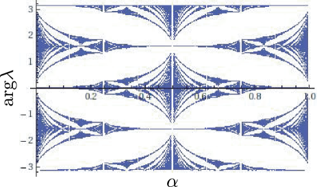
Figure 3: The self-similar and fractal structure in the inhomogeneous QW. Arguments of the eigenvalues of $CW$ (vertical axis) are plotted as a function of the parameter $\alpha=\frac{P}{4Q}$ (horizontal axis) with $Q\leq 50$. Note that, $P$ and $Q$ must be relatively prime.

Let us explain the above properties in more detail. (P1) simply means that the spectrum in Fig. 3 is symmetrical with respect to the line $\alpha=1/2$. This property can be shown as follows. Suppose that ${\vec{{\varphi}}}$ is the eigenvector of ${\sf CW}$ at the inverse period $\alpha$ with the eigenvalue $\lambda$. Then, according to Eq. (29), one obtains

$$\lambda{\varphi}(-Q;R) =(-1)^{\frac{P+1}{2}}{\varphi}(-Q+1;L),$$

$$\lambda\left(\begin{array}[]{c}{\varphi}(n;L)\\ {\varphi}(n;R)\end{array}\right) ={\hat{C}}_{n}(\alpha)\left(\begin{array}[]{c}{\varphi}(n+1;L)\\ {\varphi}(n-1;R)\end{array}\right),(n\in(-Q,Q))$$ (51)

$$\lambda{\varphi}(Q;L) =(-1)^{\frac{P+1}{2}}{\varphi}(Q-1;R),$$ (52)

where ${\hat{C}}_{n}$ is denoted as ${\hat{C}}_{n}(\alpha)$ to emphasize the argument $\alpha$. We now consider the following transformation:

$${\varphi}(n;L)\to{\varphi}(-n;R),~{}~{}~{}~{}{\varphi}(n;R)\to{\varphi}(-n;L).$$ (53)

Under this transformation, Eq. (52) becomes

$$\lambda{\varphi}(-Q;R) =(-1)^{\frac{P+1}{2}}{\varphi}(-Q+1;L),$$

$$\lambda\left(\begin{array}[]{c}{\varphi}(n;L)\\ {\varphi}(n;R)\end{array}\right) ={\hat{C}}_{n}(-\alpha)\left(\begin{array}[]{c}{\varphi}(n+1;L)\\ {\varphi}(n-1;R)\end{array}\right),(n\in(-Q,Q))$$ (58)

$$\lambda{\varphi}(Q;L) =(-1)^{\frac{P+1}{2}}{\varphi}(Q-1;R).$$ (59)

The above equations are equivalent to ${\sf CW}{\vec{{\varphi}}}=\lambda{\vec{{\varphi}}}$ at the inverse period $1-\alpha$. Therefore, the sets of eigenvalues at $\alpha$ and $1-\alpha$ are identical. Furthermore, one can construct the eigenvectors of ${\sf CW}$ at $1-\alpha$ from those at $\alpha$ using the transformation (53). (P2) implies that the spectrum is symmetrical with respect to the line ${\rm arg}(\lambda)=0$ in Fig. 3. On can easily show (P2) by taking the complex conjugate of Eq. (52) and see that ${\vec{{\varphi}}}^{*}$ is the eigenvector of ${\sf CW}$ with the eigenvalue $\lambda^{*}$. (P3) combined with (P2) gives rise to the symmetry with respect to the line ${\rm arg}(\lambda)=\pi/2$ or ${\rm arg}(\lambda)=-\pi/2$ in Fig. 3. (P3) is reminiscent of the chiral or particle-hole symmetry in the original Hofstadter problem, i.e., the eigenenergies of the Hamiltonian come in pairs $\pm E$. This property holds not only for our inhomogeneous QW but also for rather generic classes of the DTQW. To show (P3), we consider the local gauge transformation: ${\varphi}(n;\xi)\to(-1)^{n}{\varphi}(n;\xi)$. Under this transformation, ${\vec{{\varphi}}}$ becomes the eigenvector of ${\sf CW}$ with the eigenvalue $-\lambda$ according to Eq. (52). This proves (P3).

Properties (P4) and (P5) requires a more elaborate analysis. To show (P4), we first show that ${\varphi}(-Q;R)\neq 0$ if ${\vec{{\varphi}}}$ is an eigenvector of ${\sf CW}$. Suppose for the sake of contradiction that ${\varphi}(-Q;R)=0$. Using Eq. (52), it follows that ${\vec{{\varphi}}}={\vec{0}}$. But this contradicts the fact that ${\vec{{\varphi}}}$ is the eigenvector of ${\sf CW}$. Therefore, ${\varphi}(-Q;R)\neq 0$. It should be noted that $2\pi n\frac{P}{4Q}\neq\pi\ell/2$ ($\ell\in\mathbb{Z}$) for $-Q<n<Q$. We next suppose that ${\sf CW}$ has two eigenvectors ${\vec{{\varphi}}}^{(1)}$ and ${\vec{{\varphi}}}^{(2)}$ with the same eigenvalue $\lambda$. Then, we define the linear combination of them as

$${\vec{{\varphi}}}^{\prime}={{\varphi}}^{(2)}(-Q;R){\vec{{\varphi}}}^{(1)}-{{\varphi}}^{(1)}(-Q;R){\vec{{\varphi}}}^{(2)}$$ (60)

and find ${\vec{{\varphi}}}^{\prime}(-Q;R)=0$. The vector ${\vec{{\varphi}}}^{\prime}$ is also an eigenvector of ${\sf CW}$ and this contradicts the previous statement. Therefore, all the eigenvalues of ${\sf CW}$ are simple. Let us finally show the last property (P5). We first note that the product of the eigenvalues $\lambda_{k}$ $(k=1,...,4Q)$ is

$$\prod^{4Q}_{k=1}\lambda_{k}=-1$$ (61)

since $\det{\sf CW}=\det({\sf C})\det({\sf W})=-1$. Here, we have used the fact that $\det{\sf C}=1$ and $\det{\sf W}=-1$. This can be shown by an explicit calculation using Eqs. (38) and (45). Next, from (P2) and (P3), we see the eigenvalues $\lambda_{k}$ come in quadruplets $\lambda_{k}$, $\lambda^{*}_{k}$, $-\lambda_{k}$, $-\lambda^{*}_{k}$ if $\lambda_{k}$ is neither $\pm 1$ nor $\pm i$. Since $|\lambda_{k}|^{2}=1$ and Eq. (61), there exists $k$ such that $\lambda_{k}=-1$. The multiplicity of $\lambda_{k}=-1$ should be $1$ due to (P4). Then, noting the fact that the number of eigenvalues $4Q$ is a multiple of $4$, we can conclude that $\lambda_{k}=\pm i$ should also be included as the eigenvalues of ${\sf CW}$. This proves the statement (P5). Note that, the properties of the chiral symmetry (P3) and the existence of eigenvalues $\lambda=\pm 1$ are relevant to Ref. Kitagawa discussed in the standard DTQW.

V Conclusion and Outlooks

We have introduced the class of the inhomogeneous QW with self-duality inspired by the Aubry-André model Aubry_Andre . Our main result is Theorem 1. We have analytically shown that the limit distribution of the inhomogeneous QW divided by any power of time is localized at the origin when the inverse period of coins $\alpha$ is irrational number. We emphasize that our analytical solution for the localization is powerful since the round-off error is inevitable in numerical simulations. We have also numerically studied the eigenvalue distributions of the quantum walk operator $WC$ in the inhomogeneous QW with $\alpha=\frac{P}{4Q}\in\mathbb{Q}$. The obtained spectrum shows the self-similar and fractal structure similar to the Hofstadter butterfly.

In our model, the following problems remain open: First, it might be possible to experimentally realize the inhomogeneous QW in quantum optics as pointed out in Ref. Broome . Second, the recurrence property of the inhomogeneous QW has not been analytically obtained. The example of the recurrence is numerically shown in Fig. 4. Finally, we have not yet obtained the limit distribution in the case of the rational $\alpha\in\mathbb{Q}$ except for $\alpha=\frac{P}{4Q}$ with relative prime $P$ (odd integer) and $Q$. According to Ref. Cantero , the limit distribution of the DTQW is partly related to the eigenvalues of the quantum walk operator $WC$. From Fig. 3, the eigenvalues in the considering case seem to be continuous. Therefore, we propose the following conjecture as a general property of the DTQW.

Conjecture 1.

The distribution of the DTQW is not localized if the quantum walk operator $WC$ only has continuous spectra and does not have embedded eigenvalues.

This conjecture is motivated by Ref. Simon to show the property of the bound states from the spectrum of the discrete Schrödinger operator, which includes the almost Mathieu equation (1). Let us examine this conjecture for some cases in our inhomogeneous QW. It is easy to check that, in the case of $\alpha=P/2\ (P\in\mathbb{Z})$, $WC$ has a continuous spectrum and localization does not occur. In this case, the coin state is unchanged up to the phase factor since the coin operator is always $\left(\begin{array}[]{cc}1&0\\ 0&1\end{array}\right)$ or $\left(\begin{array}[]{cc}-1&0\\ 0&-1\end{array}\right)$. Therefore, the quantum walker does not undergo reflection at any point. Furthermore, in the case of $\alpha=1/6$, Linden and Sharam showed that the standard deviation is proportional to the time variable $t$ for a sufficient large $t$ Linden . These facts partially support the above conjecture.

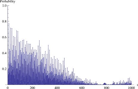
Figure 4: Recurrence property of the inhomogeneous QW with the initial coin state $(|{L}\rangle+|{R}\rangle)/\sqrt{2}$ and the inverse period $\alpha=\pi/2$. The numerically obtained probabilities at the origin are shown up to $1000$ time steps. Note that the probability at the origin must be zero when the step $t$ is odd.

References

- (1) S. P. Gudder, Quantum Probability (Academic Press Inc., CA, 1988).
- (2) Y. Aharonov, L. Davidovich, and N. Zagury, Phys. Rev. A 48, 1687 (1993).
- (3) D. Meyer, J. Stat. Phys. 85, 551 (1996).
- (4) A. M. Childs, Phys. Rev. Lett. 102, 180501 (2009).
- (5) N. B. Lovett, S. Cooper, M. Everitt, M. Trevers, and V. Kendon, Phys. Rev. A 81, 042330 (2010).
- (6) N. Shenvi, J.Kempe, and K. Birgitta Whaley, Phys. Rev. A 67, 052307 (2003).
- (7) H. Buhrman and R. Spalek, in Proc. 17th ACM-SIAM Symposium on Discrete Algorithms (Society for Industrial and Applied Mathematics, Philadelphia, 2006), p. 880.
- (8) F. Magniez and A. Nayak, Algorithmica 48, 221 (2007).
- (9) A. Ambainis, SIAM Journal on Computing 37, 210 (2007).
- (10) F. Magniez, M. Santha, and M. Szegedy, SIAM Journal of Computing 37, 413 (2007).
- (11) T. Kitagawa, M. S. Rudner, E. Berg, and E. Demler, arXiv:1003.1729.
- (12) C. M. Chandrashekar and R. Laflamme, Phys. Rev. A 78, 022314 (2008).
- (13) T. Oka, N. Konno, R. Arita, and H. Aoki, Phys. Rev. Lett. 94, 100602 (2005).
- (14) Y. Shikano, K. Chisaki, E. Segawa, and N. Konno, Phys. Rev. A 81, 062129 (2010).
- (15) G. S. Engel, T. R. Calhoun, E. L. Read, T.-K. Ahn, T. Mančal, Y.-C. Cheng, R. E. Blankenship, and G. R. Fleming, Nature 446, 782 (2007).
- (16) M. Mohseni, P. Rebentrost, S. Lloyd, and A. Aspuru-Guzik, J. Chem. Phys. 129, 174106 (2008).
- (17) J. Kempe, Contemp. Phys. 44, 307 (2003).
- (18) V. Kendon, Math. Struct. in Comp. Sci. 17, 1169 (2007).
- (19) N. Konno, in Quantum Potential Theory, Lecture Notes in Mathematics Vol. 1954, edited by U. Franz and M. Schurmann (Springer-Verlag, Heidelberg, 2008), pp.309-452.
- (20) S. E. Venegas-Andraca, Quantum Walks for Computer Scientists (Morgan and Claypool, 2008).
- (21) N. Inui, N. Konno, and E. Segawa, Phys. Rev. E 72, 056112 (2005).
- (22) N. Inui, and N. Konno, Physica A 353, 133 (2005).
- (23) M. McGettrick, Quantum Inf. Comp. 10, 0509 (2010).
- (24) A. Joye and M. Merkli, arXiv:1004.4130.
- (25) C. Liu and N. Petulante, Phys. Rev. A 79, 032312 (2009).
- (26) N. Konno and E. Segawa, arXiv:1008.5109.
- (27) K. Chisaki, N. Konno, and E. Segawa, arXiv:1009.1306.
- (28) A. Romanelli, Physica A 388, 3985 (2009).
- (29) T. D. Mackay, S. D. Bartlett, L. T. Stephenson, and B. C. Sanders, J. Phys. A 35, 2745 (2002).
- (30) B. Tregenna, W. Flanagan, R. Maile, and V. Kendon, New J. Phys. 5, 83 (2003).
- (31) N. Inui, Y. Konishi, and N. Konno, Phys. Rev. A 69, 052323 (2004).
- (32) K. Watabe, N. Kobayashi, M. Katori, and N. Konno, Phys. Rev. A 77, 062331 (2008).
- (33) K. Chisaki, M. Hamada, N. Konno, and E. Segawa, Interdisciplinary Information Sciences 15, 423 (2009).
- (34) A. Wójcik, T. Łuczak, P. Kurzyński, A. Grudka, and M. Bednarska, Phys. Rev. Lett. 93, 180601 (2004).
- (35) M. Štefaňák, I. Jex, and T. Kiss, Phys. Rev. Lett. 100, 020501 (2008).
- (36) M. Štefaňák, T. Kiss, and I. Jex, Phys. Rev. A 78, 032306 (2008); New J. Phys. 11, 043027 (2009).
- (37) C. M. Chandrashekar, Cent. Eur. J. Phys., 8, 979 (2010).
- (38) X.-P. Xu, arXiv:1003.1822.
- (39) N. Konno, Quantum Inf. Proc. 8, 387 (2009).
- (40) N. Konno, Quantum Inf. Proc., 9, 405 (2010).
- (41) N. Linden and J. Sharam, Phys. Rev. A 80, 052327 (2009).
- (42) S. Aubry and G. André, Ann. Israel Phys. Soc. 3, 133 (1980).
- (43) J. Bellissard, and B. Simon, J. Funct. Anal. 48, 408 (1982).
- (44) J. B. Sokoloff, Phys. Rep. 126, 189 (1985).
- (45) M. Ya. Azbel, Zh. Eksp. Teor. Fiz. 46, 929 (1964). [Sov. Phys.-JETP 19, 634 (1964).]
- (46) D. R. Hofstadter, Phys. Rev. B 14, 2239 (1976).
- (47) M. Kohmoto, Phys. Rev. Lett. 51, 1198 (1983).
- (48) C. Tang, and M. Kohmoto, Phys. Rev. B 34, 2041 (1986).
- (49) P. B. Wiegmann and A. V. Zabrodin, Phys. Rev. Lett. 72, 1890 (1994); Nucl. Phys. B422, 495 (1994).
- (50) Y. Hatsugai, M. Kohmoto, and Y.-S. Wu, Phys. Rev. Lett. 73, 1134 (1994); Phys. Rev. B 53, 9697 (1996).
- (51) A. G. Abanov, J. C. Talstra, and P. B. Wiegmann, Phys. Rev. Lett. 81, 2112 (1998); Nucl. Phys. B525, 571 (1998).
- (52) A. Ambainis, E. Bach, A. Nayak, A. Vishwanath, and J. Watrous, in Proceedings of the 33rd Annual ACM Symposium on Theory of Computing (STOC’01) (ACM Press, New York, 2001), pp. 37 - 49.
- (53) G. Grimmett, S. Janson, and P. F. Scudo, Phys. Rev. E. 69, 026119 (2004).
- (54) B. Fristedt and L. Gray, A Modern Approach to Probability Theory (Birkhaäuser, Boston, 1997).
- (55) Convergence in distribution is also used in the central limit theorem; the discrete distribution can be approximated by the continuous distribution. Therefore, the domain of the probability density function for the limit distribution is the real number . Please see Ref. (FG, , Part 3) for the formal definitions.
- (56) G. H. Hardy and E. M. Wright, An Introduction to the Theory of Number (Clarendon Press, Oxford, 1979).
- (57) M. A. Broome, A. Fedrizzi, B. P. Lanyon, I. Kassal, A. Aspuru-Guzik, and A. G. White, Phys. Rev. Lett. 104, 153602 (2010).
- (58) M. J. Cantero, L. Moral, F. A. Grünbaum, and L. Velázquez, Commun. Pure Appl. Math. 63, 464 (2010).
- (59) D. Damanik, R. Killip, and B. Simon, Commun. Math. Phys. 258, 741 (2005).