Constraints from primordial black hole formation at the end of inflation
Abstract
Primordial black hole (PBH) abundance limits constrain the primordial power spectrum, and hence models of inflation, on scales far smaller than those probed by cosmological observations. Single field inflation models which are compatible with all cosmological data can have large enough perturbations on small scales to overproduce PBHs, and hence be excluded. The standard formulae for the amplitude of perturbations do not hold for modes that exit the horizon close to the end of inflation however. We use a modified flow analysis to identify models of inflation where the amplitude of perturbations on small scales is large. For these models we then carry out a numerical evolution of the perturbations and use the PBH constraints on the power spectrum to eliminate models which overproduce PBHs. Significant PBH formation can occur in models in which inflation can continue indefinitely and is ended via a secondary mechanism. We demonstrate that PBHs constrain these types of inflation models and show that a numerical evaluation of the power spectrum decreases the number of otherwise viable models of inflation.
pacs:
98.80.CqI Introduction
Primordial black holes (PBHs) can form in the early Universe via the collapse of large density perturbations Carr:1974nx ; Carr:1975qj . There are tight constraints on the abundance of PBHs formed from their present day gravitational effects and the consequences of their evaporation. These limits can be used to constrain the power spectrum of the primordial density, or curvature, perturbations. The PBH constraints on the curvature power spectrum are fairly weak, being many orders of magnitude larger than the measurements on cosmological scales. They do, however, apply over a very wide range of scales and therefore provide a useful constraint on models of inflation. Peiris and Easther Peiris:2008be have shown that there are single field inflation models, which are compatible with all cosmological observations, for which the perturbation amplitude on small scales is large enough to produce a significant density of PBHs.
For scales which exit the horizon close to the end of inflation the standard (Stewart-Lyth Stewart:1993bc ) formulae for the amplitude of perturbations do not hold. Leach and Liddle Leach:2000yw carried out a numerical calculation of the evolution of perturbations for a quadratic inflationary potential. They found that the perturbations on scales which exit the horizon close to the end of inflation were roughly an order of magnitude larger than predicted by the Stewart-Lyth formula (see also Ref. Bugaev:2008bi ). Therefore to fully exploit the power of PBH constraints on inflation models, a numerical calculation of the amplitude of perturbations on small scales is required. It has recently been shown Lyth:2005ze ; Zaballa:2009xb that PBHs can also form on scales which never leave the horizon. We do not consider this possibility here.
In this paper we use a modified flow analysis to identify inflation models where the perturbations at the end of inflation may be large enough for primordial black holes to be overproduced. For these models we carry out a numerical evolution of the primordial perturbations and use the PBH constraints on the power spectrum to eliminate models which overproduce PBHs. We describe the modified flow analysis in Sec. II.1 and the evolution of perturbations and the calculation of the power spectrum in Sec. II.2. We apply the primordial black hole abundance constraints and present our results in Sec. III and conclude with discussion in Sec. IV.
II Method
II.1 Flow equations approach
We consider the Hubble slow roll-parameters Salopek:1990jq :
| (1) | |||||
| (2) |
where is the Planck mass and ′ denotes differentiation with respect to the scalar field, . The flow equations Hoffman:2000ue ; Kinney:2002qn encode the variation of the slow-roll parameters in terms of the number of e-foldings from the end of inflation, and provide a method for stochastically generating inflation models:
| (3) | |||||
| (4) | |||||
where and .
Following Kinney Kinney:2002qn we randomly chose ‘initial’ values for the slow-roll parameters and , the number of e-foldings between cosmological scales exiting the horizon and the end of inflation, in the ranges:
| (6) |
truncating the hierarchy at . We then evolve the flow equations forward in time () from until either or inflation ends with . In the former case we calculate the cosmological observables, the spectral index, , its running, , and the scalar to tensor ratio, , using the initial values of the slow-roll parameters Kinney:2002qn :
| (7) | |||||
| (8) | |||||
| (9) |
where and . In the latter case we evolve the flow equations backward e-folds and calculate the cosmological observables at this point. In some cases inflation also ends when evolving backwards before e-folds are achieved. These models are incapable of supporting the required amount of inflation and are discarded.
Our algorithm differs from that originally proposed by Kinney Kinney:2002qn in how we handle models chosen from the initial hierarchy that are destined to inflate forever, , but do not reach this limit within e-foldings. In the original flow algorithm in this case the cosmological observables are calculated at the late-time fixed point i.e. the model is forced to evolve to its asymptotic limit. In this limit the running of the spectral index is negligible. Therefore for models which are compatible with the WMAP 7 year measurement of the spectral index, Komatsu:2010fb , the amplitude of the curvature perturbations can not be large on any scale and PBHs are never formed in significant numbers Chongchitnan:2006wx . Following Peiris and Easther Peiris:2008be , we do not force these models to evolve to their asymptotic limit but instead terminate them once e-folds of inflation have occurred. At this point it is assumed that another mechanism, for example a second-field such as in hybrid inflation Linde:1993cn , terminates inflation. With this treatment some of these models are consistent with the WMAP measurements of the spectral index and its running, but have perturbations on small scales which may be large enough to over-produce PBHs Peiris:2008be ; Alabidi:2009bk ; Kohri:2007qn ; Bugaev:2008gw .
II.2 Perturbation calculation
The evolution of inflationary curvature perturbations, , is carried out using the Mukhanov variable Mukhanov:1990me , , where
| (10) |
The Fourier modes, , evolve according to a Klein-Gordon equation with a time-varying effective mass:
| (11) |
where is conformal time, , and
| (12) | |||||
At early times, , when a mode is well within the horizon, , the initial condition for , is taken to be the Bunch-Davies vacuum state,
| (13) |
In the superhorizon limit, , eq. (11) has a growing mode solution , so that the curvature perturbation ‘freezes out’ and becomes constant. The power-spectrum of the curvature perturbations can thus be calculated as
| (14) |
Eq. (11) can be solved exactly for the special case of power-law inflation. The commonly used Stewart-Lyth formula is found via a slow-roll expansion around this exact solution Stewart:1993bc :
| (15) |
where . This expression gives the power spectrum in the asymptotic superhorizon limit, , in terms of the Hubble parameter and slow-roll parameters evaluated at horizon crossing Grivell:1996sr . It is valid provided that the slow-roll approximation holds (specifically that the slow-roll parameters are slowly varying around horizon crossing) and the asymptotic limit is reached before inflation ends Huang:2000bh . For modes which exit the horizon close to the end of inflation the asymptotic limit will not be reached, and the slow-roll approximation may also be violated.
Leach & Liddle Leach:2000yw investigated this for a simple quadratic chaotic inflation model. They found that for scales that exit the horizon very close to the end of inflation the power spectrum is roughly an order of magnitude larger than that found using the Stewart-Lyth expression. In other words, analytic calculations can significantly underestimate the amplitude of perturbations and hence the abundance of PBHs formed. Therefore, a numerical calculation of the perturbation evolution is required to accurately compute the primordial power spectrum on the very smallest scales.
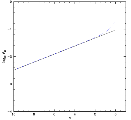
We use a modified version of the Inflation v2 module (written by Lesgourgues & Valkenburg) Lesgourgues:2007aa to carry out an accurate numerical calculation of the evolution of perturbations. Fig. 1 shows the power spectrum of curvature perturbations of an example inflation model generated using the modified horizon flow formalism. The power spectrum on large scales is compatible with the WMAP 7 year data, while the perturbations on small scales are sufficiently large that PBHs may be over-produced. The Stewart-Lyth calculation is in good agreement with the numerical calculation until the final few e-folds of inflation. On these small scales, the assumptions that are employed in the Stewart-Lyth calculation break down, and the numerical calculation finds a significant enhancement of the amplitude of the perturbations.
III Results


We use the modified flow algorithm described in sec. II.1 to generate a large ensemble (250,000) of inflation models. In fig. 2 (top row) we plot the cosmological observables for all models which are able to sustain the required number of e-foldings of inflation, . In around of the models inflation ends naturally via and these largely populate the concentrated diagonal feature seen in the left hand plots as well as the line (c.f. Ref. Kinney:2002qn ). In the remaining of models, and it is assumed, c.f. Ref. Peiris:2008be , that a secondary mechanism, such as hybrid inflation, acts to end inflation in these cases. Large positive running is in principle allowed (see top right plot), however these models may have large amplitude perturbations on small scales and hence overproduce PBHs.
To apply the PBH constraints we use the Stewart-Lyth expression for the power spectrum, eq. (15), to identify inflation models where the amplitude of the perturbations on small scales which exit the horizon close to the end of inflation is large, and may lead to the over-production of PBHs. For these models, we then carry out an accurate numerical evolution of the primordial perturbations, as described in Sec. II.2.
The PBH abundance constraints have recently been compiled and updated in Refs. Josan:2009qn ; Carr:2009jm . The resulting constraints on the amplitude of the power spectrum are typically in the range with some scale dependence Josan:2009qn . To be conservative we use the constraint . The bottom row of fig. 2 shows the cosmological observables for the models which remain once those which over-produce PBHs are excluded. The of the original models for which inflation ends naturally generally have on all scales and so are unaffected by the PBH constraints. Of the remaining models, in which inflation continues indefinitely in the absence of a secondary mechanism, are excluded by PBH overproduction. Of the models initially generated, only approximately end via a secondary mechanism and do not overproduce PBHs. With an accurate numerical calculation of the perturbations the number of these models decreases by approximately . Large positive running is now excluded as expected (see bottom-right plot).
Cosmological constraints on eliminate a significant fraction of the models generated using flow algorithms Kinney:2002qn . A full MCMC analysis of cosmological data is beyond the scope of this work, however a simple application of the observational constraints shows that a significant fraction of cosmologically viable models are excluded by PBH constraints. Of the models generated using our modified flow analysis which have cosmological observables within the 3 ranges found by WMAP7 Komatsu:2010fb are excluded by PBH over-production. This illustrates that in the era of precision cosmological measurements PBH still provide a powerful constraint on inflation models.
IV Conclusions
We have applied constraints on the primordial power spectrum from the overproduction of primordial black holes to inflation models generated by a modified flow algorithm. The amplitude of inflationary perturbations is usually calculated using the Stewart-Lyth Stewart:1993bc expression, however for scales which exit the horizon close to the end of inflation the assumptions underlying this expression are violated. A numerical calculation is therefore required, and the amplitude of the perturbations on small scales can be significantly enhanced Leach:2000yw ; Bugaev:2008bi . The models generated by the modified flow algorithm which end naturally (roughly of the total) generally have a red spectrum of perturbations on all scales and so are unaffected by PBH constraints. The remaining of models equations have a late time attractor with and it is assumed that an auxiliary mechanism terminates inflation. The majority of these models are however excluded due to PBH over-production. The number of viable models decreases if the power spectrum is calculated numerically. Of the models generated using our modified flow analysis which have cosmological observables within the 3 ranges found by WMAP7 Komatsu:2010fb are excluded by PBH over-production.
We conclude that PBH constraints provide a significant constraint on models of inflation. Furthermore to exploit their full power an accurate numerical calculation of the amplitude of primordial perturbations on small scales, which exit the horizon close to the end of inflation, is required.
Acknowledgements.
We are grateful to Andrew Liddle and Will Hartley for useful discussions and acknowledge the use of the Inflation v2 module (written by Julien Lesgourgues and Wessel Valkenburg). AJ is supported by the University of Nottingham, AMG is supported by STFC.References
- (1) B. J. Carr and S. W. Hawking Mon. Not. Roy. Astron. Soc. 168 (1974) 399–415.
- (2) B. J. Carr Astrophys. J. 201 (1975) 1–19.
- (3) H. V. Peiris and R. Easther JCAP 0807 (2008) 024 [arXiv:0805.2154].
- (4) E. D. Stewart and D. H. Lyth Phys. Lett. B302 (1993) 171–175 [arXiv:gr-qc/9302019].
- (5) S. M. Leach and A. R. Liddle Phys. Rev. D63 (2001) 043508 [arXiv:astro-ph/0010082].
- (6) E. Bugaev and P. Klimai Phys. Rev. D78 (2008) 063515 [arXiv:0806.4541].
- (7) D. H. Lyth, K. A. Malik, M. Sasaki and I. Zaballa JCAP 0601 (2006) 011 [arXiv:astro-ph/0510647].
- (8) I. Zaballa and M. Sasaki arXiv:0911.2069.
- (9) D. S. Salopek and J. R. Bond Phys. Rev. D42 (1990) 3936–3962.
- (10) M. B. Hoffman and M. S. Turner Phys. Rev. D64 (2001) 023506 [arXiv:astro-ph/0006321].
- (11) W. H. Kinney Phys. Rev. D66 (2002) 083508 [arXiv:astro-ph/0206032].
- (12) E. Komatsu et. al. arXiv:1001.4538.
- (13) S. Chongchitnan and G. Efstathiou JCAP 0701 (2007) 011 [arXiv:astro-ph/0611818].
- (14) A. D. Linde Phys. Rev. D49 (1994) 748–754 [arXiv:astro-ph/9307002].
- (15) L. Alabidi and K. Kohri Phys. Rev. D80 (2009) 063511 [arXiv:0906.1398].
- (16) K. Kohri, D. H. Lyth and A. Melchiorri JCAP 0804 (2008) 038 [arXiv:0711.5006].
- (17) E. Bugaev and P. Klimai Phys. Rev. D79 (2009) 103511 [arXiv:0812.4247].
- (18) V. F. Mukhanov, H. A. Feldman and R. H. Brandenberger Phys. Rept. 215 (1992) 203–333.
- (19) I. J. Grivell and A. R. Liddle Phys. Rev. D54 (1996) 7191–7198 [arXiv:astro-ph/9607096].
- (20) D. H. Huang, W. B. Lin and X. M. Zhang Phys. Rev. D62 (2000) 087302 [arXiv:hep-ph/0007064].
- (21) J. Lesgourgues, A. A. Starobinsky and W. Valkenburg JCAP 0801 (2008) 010 [arXiv:0710.1630].
- (22) A. S. Josan, A. M. Green and K. A. Malik Phys. Rev. D79 (2009) 103520 [arXiv:0903.3184].
- (23) B. Carr, K. Kohri, Y. Sendouda and J. Yokoyama arXiv:0912.5297.