When Two Trees Go to War

Abstract

Rooted phylogenetic networks are often constructed by combining trees, clusters, triplets or characters into a single network that in some well-defined sense simultaneously represents them all. We review these four models and investigate how they are related. In general, the model chosen influences the minimum number of reticulation events required. However, when one obtains the input data from two binary trees, we show that the minimum number of reticulations is independent of the model. The number of reticulations necessary to represent the trees, triplets, clusters (in the softwired sense) and characters (with unrestricted multiple crossover recombination) are all equal. Furthermore, we show that these results also hold when not the number of reticulations but the level of the constructed network is minimised. We use these unification results to settle several complexity questions that have been open in the field for some time. We also give explicit examples to show that already for data obtained from three binary trees the models begin to diverge.

1 Introduction

Consider a set of taxa ${\mathcal{X}}$. A rooted phylogenetic network on ${\mathcal{X}}$ is a rooted directed acyclic graph in which the outdegree-zero nodes (the leaves) are bijectively labelled by ${\mathcal{X}}$. It is common to identify a leaf with the taxon it is labelled by and it is usually assumed that there are no nodes with indegree and outdegree one; we adopt both conventions. Nodes with indegree at least two are called reticulations. The edges entering a reticulation are called reticulation edges. Nodes that are not reticulations are called tree nodes. A phylogenetic network is called binary if all reticulations have indegree two and outdegree one and all other nodes have outdegree zero or two.

One of the main challenges in phylogenetics is to reconstruct phylogenetic networks from biological data of currently living organisms. The reticulations in a phylogenetic network are of special biological interest. These nodes represent “reticulate” evolutionary phenomena like hybridisation, recombination or lateral (horizontal) gene transfer. Motivated by the parsimony principle, a phylogenetic network with fewer reticulations is often preferred over a network with more reticulations, when both networks represent the available data equally well.

Thus, we define the following fundamental problem MinRet. Given some set ${\mathcal{D}}$ of data describing some set ${\mathcal{X}}$ of taxa, find a phylogenetic network on ${\mathcal{X}}$ that “represents” ${\mathcal{D}}$ and contains a minimum number of reticulations over all phylogenetic networks on ${\mathcal{X}}$ representing ${\mathcal{D}}$. We consider three specific variants of this problem: MinRetTrees, MinRetTriplets and MinRetClusters, for data ${\mathcal{D}}$ consisting of trees, triplets and clusters respectively.

The following subtlety has to be taken into account when reticulations with indegree higher than two are considered. When counting such reticulations, indegree-$d$ reticulations are counted $d-1$ times, because such reticulations represent $d-1$ reticulate evolutionary events (of which the order is not specified). Hence, using $\delta^{-}(v)$ to denote the indegree of a node $v$, we formally define the number of reticulations in a phylogenetic network $N=(V,E)$ as

$$\sum_{\begin{subarray}{c}v\in V:\delta^{-}(v)>0\end{subarray}}(\delta^{-}(v)-1)=|E|-|V|+1\enspace.$$

Instead of minimizing the total number of reticulations in a network, another possibility is to minimize the number of reticulations in each nontrivial biconnected component (informally: tangled part) of a network. Formally, a biconnected component is a maximal subgraph that cannot be disconnected by removing a single node. A biconnected component is trivial if it is equal to a single edge and nontrivial otherwise. For $k\in\mathbb{N}$, a phylogenetic network is called a level-$k$ network if each nontrivial biconnected component contains at most $k$ reticulations. See Figure 1 for an example of a phylogenetic network with four reticulations. This is a level-3 network, because each nontrivial biconnected component contains at most three reticulations.

Figure 1: A level-3 phylogenetic network with four reticulations. Nontrivial biconnected components are encircled by dashed lines. Reticulations are unfilled and colored red. Reticulation edges are also indicated in red.

This leads to the definition of the following MinLev variant of the fundamental problem. Given some set ${\mathcal{D}}$ of data describing some set ${\mathcal{X}}$ of taxa, find a level-$k$ phylogenetic network that “represents” ${\mathcal{D}}$ such that $k$ is as small as possible. There are again three versions: MinLevTrees, MinLevTriplets and MinLevClusters, for data ${\mathcal{D}}$ consisting of trees, triplets and clusters respectively.

The definition of “represents” heavily depends on the nature of the data in ${\mathcal{D}}$. We will discuss four types of data: trees, triplets, clusters and binary characters. Throughout the paper we assume a fixed set ${\mathcal{X}}$ of taxa.

1.1 Trees

A phylogenetic tree on ${\mathcal{X}}$ is a phylogenetic network on ${\mathcal{X}}$ without reticulations. There exist numerous methods that construct phylogenetic trees, for example from DNA data. These methods include Maximum Likelihood, Maximum Parsimony, Bayesian- and distance-based methods like Neighbor Joining. When phylogenetic trees are constructed for several parts of the genome separately (e.g. several genes), one often obtains a number of different phylogenetic trees. The same can occur when several phylogenetic trees are constructed using different methods.

Thus, given a number of phylogenetic trees, it is interesting to find a phylogenetic network that “represents” each of them. This is formalized by the notion of “display” as follows. A phylogenetic tree $T$ is displayed by a phylogenetic network $N$ if $T$ can be obtained from some subtree of $N$ by suppressing nodes with indegree one and outdegree one (i.e. if some subtree of $N$ is a subdivision of $T$). See Figure 2 for an example.

For a set ${\mathcal{T}}$ of phylogenetic trees on ${\mathcal{X}}$, we define:

• $r_{t}({\mathcal{T}})$ as the minimum number of reticulations in any phylogenetic network on ${\mathcal{X}}$ that displays each tree in ${\mathcal{T}}$ and

• $\ell_{t}({\mathcal{T}})$ as the minimum $k$ such that there exists a level-$k$ phylogenetic network on ${\mathcal{X}}$ that displays each tree in ${\mathcal{T}}$.

The computation of $r_{t}$ has received much attention in the literature. For two binary trees on the same taxon set the problem is NP-hard and APX-hard [4] although on the positive side it is fixed-parameter tractable in $r_{t}$ [3][2]; [22] offers a good overview of these and related results. These algorithmic insights have been translated into the software HybridNumber [2] and its more advanced successor HybridInterleave [6]. These programs compute $r_{t}$ exactly for two binary trees on the same taxon set. The program SPRDist [37] solves the same problem (using integer linear programming) and the program PIRN [35] can compute lower and upper bounds on $r_{t}$ for any number of binary trees on the same taxon set. In [15] a polynomial-time algorithm is described that constructs a level-1 phylogenetic network that displays all trees and has a minimum number of reticulations, if such a network exists.

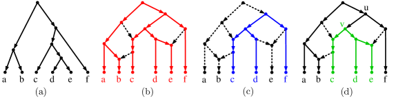
Figure 2: A phylogenetic tree $T$ (a) and a phylogenetic network $N$ (b,c,d); (b) illustrates in red that $N$ displays $T$ (edges not in the subdivision are dashed); (c) illustrates in blue that $N$ is consistent with the triplet $cd|f$ from $T$ (edges not in the embedding are again dashed); (d) illustrates in green that $N$ represents cluster $\{c,d,e\}$ from $T$ in the softwired sense (dashed reticulation edges are “switched off”).

1.2 Triplets

A (rooted) triplet on ${\mathcal{X}}$ is a binary phylogenetic tree on a size-3 subset of ${\mathcal{X}}$. We use $xy|z$ to denote the triplet with taxa $x,y$ on one side of the root and $z$ on the other side of the root. Triplets can be constructed using any of the methods for constructing phylogenetic trees (using a fourth taxon as an outgroup in order to root the triplet). Alternatively, one can first construct one or more phylogenetic trees and subsequently find the set of triplets that are contained in these trees. The main motivation for the latter approach is that representing all triplets might require fewer reticulations than representing the entire trees.

This can be formalised by using the notion of display introduced above. For triplets, often “consistent with” is used instead of “displayed by”. A triplet $xy|z$ is consistent with a phylogenetic network $N$ (and $N$ is consistent with $xy|z$) if $xy|z$ is displayed by $N$. See Figure 2 for an example. Given a phylogenetic tree $T$ on ${\mathcal{X}}$, we let $Tr(T)$ denote the set of all rooted triplets on ${\mathcal{X}}$ that are consistent with $T$. For a set of phylogenetic trees $\mathcal{T}$, we let $Tr(\mathcal{T})$ denote the set of all rooted triplets that are consistent with some tree in $\mathcal{T}$, i.e. $Tr(\mathcal{T})=\bigcup_{T\in\mathcal{T}}Tr(T)$.

For a set ${\mathcal{R}}$ of triplets on ${\mathcal{X}}$, we define:

• $r_{tr}({\mathcal{R}})$ as the minimum number of reticulations in any phylogenetic network on ${\mathcal{X}}$ that is consistent with each triplet in ${\mathcal{R}}$ and

• $\ell_{tr}({\mathcal{R}})$ as the minimum $k$ such that there exists a level-$k$ phylogenetic network on ${\mathcal{X}}$ that is consistent with each triplet in ${\mathcal{R}}$.

Throughout the article we will write $r_{tr}(\mathcal{T})$ and $\ell_{tr}(\mathcal{T})$ as abbreviations for $r_{tr}(Tr(\mathcal{T}))$ and $\ell_{tr}(Tr(\mathcal{T}))$ respectively.

A triplet set $\mathcal{R}$ on $\mathcal{X}$ is said to be dense when, for every three distinct taxa $x,y,z\in\mathcal{X}$, at least one of $xy|z,xz|y,yz|x$ is in $\mathcal{R}$ [16]. Given a dense triplet set, [16][17] describe a polynomial-time algorithm that constructs a level-1 network displaying all triplets, if such a network exists. The algorithm [30] can be used to find such a network that also minimizes the number of reticulations, and this is available as the program Marlon [28]. These results have later been extended to level-2 [27][30] (see also the program Level2 [26]) and more recently to level-$k$, for all $k\in\mathbb{N}$ [25]. The program Simplistic [29][30] can be used to construct (simple) networks of arbitrary level (again, assuming density).

1.3 Clusters

A cluster on ${\mathcal{X}}$ is a proper subset of ${\mathcal{X}}$. Clusters can be obtained from morphological data (e.g. species with wings, species with eight legs, etc.) or from phylogenetic trees. The latter approach has a similar motivation as in triplet methods. The clusters from the trees might be representable using fewer reticulations than that would be necessary to represent the trees themselves. In addition, the clusters described by a phylogenetic tree are biologically the most interesting features of the tree, because they describe putative monophyletic groups of species (clades).

We use $Cl(T)$ to denote the set of clusters of a phylogenetic tree $T$, i.e. for each edge $(u,v)$ of $T$, the set $Cl(T)$ contains a cluster consisting of those taxa that are reachable by a directed path from $v$. For a set ${\mathcal{T}}$ of phylogenetic trees, we define $Cl({\mathcal{T}})=\bigcup_{T\in{\mathcal{T}}}Cl(T)$.

Similar to tree- and triplet methods, the general aim of cluster methods is to construct a phylogenetic network that “represents” some set of input clusters. There are two different notions of “representing” for clusters: the “hardwired” and the “softwired” sense. Given a cluster $C\subset{\mathcal{X}}$ and a phylogenetic network $N$ on ${\mathcal{X}}$, we say that $N$ represents $C$ in the hardwired sense if there exists an edge $(u,v)$ in $N$ such that $C$ is the set of taxa reachable from $v$ by a directed path [13].

The definition of “representing” in the “softwired sense” is longer but biologically more relevant. We say that $N$ represents $C$ in the softwired sense if there exists an edge $(u,v)$ in $N$ such that $C$ is the set of taxa reachable from $v$ by a directed path, when for each reticulation $r$ exactly one its incoming edges is “switched on” and all other edges entering $r$ are “switched off” (see Figure 2). As a direct consequence, $C$ is represented by $N$ in the softwired sense if and only if there exists a phylogenetic tree $T$ on ${\mathcal{X}}$ that is displayed by $N$ and has $C\in Cl(T)$. In this article, we do not consider cluster representation in the hardwired sense and therefore often write “represents” as short for “represents in the softwired sense”.

For a set of clusters ${\mathcal{C}}$ on ${\mathcal{X}}$, we define:

• $r_{c}({\mathcal{C}})$ as the minimum number of reticulations in any phylogenetic network on ${\mathcal{X}}$ that represents all clusters in ${\mathcal{C}}$ in the softwired sense and

• $\ell_{c}({\mathcal{C}})$ as the minimum $k$ such that there exists a level-$k$ phylogenetic network on ${\mathcal{X}}$ that represents all clusters in ${\mathcal{C}}$ in the softwired sense.

We write $r_{c}({\mathcal{T}})$ as shorthand for $r_{c}(Cl({\mathcal{T}}))$ and $\ell_{c}({\mathcal{T}})$ as shorthand for $\ell_{c}(Cl({\mathcal{T}}))$.

A network is a galled network if it contains no path between two reticulations that is contained in a single biconnected component. In [11] and [14] an algorithm is described for constructing a galled network representing $\mathcal{C}$ in the softwired sense. In [33] the algorithm Cass [32] is presented which aims at constructing a low-level network that represents $\mathcal{C}$. Cass always returns a network representing all input clusters and, when $\ell_{c}({\mathcal{C}})\leq 2$, it is guaranteed to compute $\ell_{c}$ exactly. Alongside the algorithms from [14][11][13] Cass is available as part of the program Dendroscope [12].

1.4 Binary character data

Within the field of population genomics the literature on phylogenetic networks has evolved along a slightly different route to the literature on trees, triplets and clusters. At the level of populations the principle reticulation event is the recombination, and in this context phylogenetic networks are sometimes called recombination networks. To avoid repetition we refer to [10][8][36] for background and definitions. In this article we will always assume that recombination networks are constructed from binary character data and that the root sequence is the all-0 sequence i.e. we are dealing with the “root known” variant of the problem. We assume thus that the input is a binary $n\times m$ matrix $M$.

The basic definition given in [10] is for the unrestricted multiple crossover variant of the recombination network model. Stated informally this means that, at each reticulation, each character can freely “choose” from which of its parents it inherits its value. This is quite different to the single crossover variant which has received far more attention in the literature. In the single crossover variant the sequence at a reticulation is forced to obtain a prefix from one of its parents, and a suffix from the other, thus modelling chromosomal crossover.

For a binary matrix $M$, we define:

• $r_{sc}(M)$ as the minimum number of reticulations required by a recombination network that represents $M$, assuming the single crossover variant and an all-0 root, and

• $r_{uc}(M)$ as the minimum number of reticulations required by a recombination network that represents $M$, assuming the unrestrained multiple crossover variant and an all-0 root.

Given that the latter is a relaxation of the former, it is immediately clear that for any input $M$,

$$r_{uc}(M)\leq r_{sc}(M).$$ (1)

In [34] it was claimed that it is NP-hard to compute $r_{uc}$. However, [4] subsequently discovered that the proof in [34] was partially incorrect and modified it to prove that computation of $r_{sc}$ is NP-hard.

There are some definitional subtleties when trying to map between the model of [10] and the other models summarised in this article. Some differences between the models are rather arbitrary and minor and thus easy to overcome, and we do not discuss them here. In this article we restrict ourself to a more fundamental comparison concerning (under an appropriate transformation) the values $r_{sc}$, $r_{uc}$ and $r_{c}$.

The problem of computing $r_{sc}$ (in defiance of its NP-hardness) has attracted much attention. Articles such as [10][8][36][24][19] give a good overview of the methods in use. Much energy has been invested in computing lower bounds for $r_{sc}$ (e.g. the program HapBound [24]), and some lower bounding techniques also produce valid lower bounds for $r_{uc}$ (e.g. [10]). Programs such as Shrub [24] produce upper bounds on $r_{sc}$, and Beagle [19] uses integer linear programming to compute $r_{sc}$ exactly (for small instances). The programs HapBound-GC and Shrub-GC compute lower and upper bounds on a value that lies somewhere between $r_{sc}$ and $r_{uc}$ [23]. As in other areas of the phylogenetic network literature the problem of computing $r_{sc}$ in a topologically constrained space of networks [9] has also been considered.

1.5 Summary of Results

In this article, we study how several methods for constructing phylogenetic networks are related. We begin by clarifying the relationship between phylogenetic networks that represent clusters in the softwired sense and recombination networks that represent binary character data. We explain that the two models are equivalent when unrestricted multiple crossover recombination is considered but fundamentally different when single crossover recombination is used. This clarification is necessary to place the main results from this article in the correct context.

We then turn to the problem of constructing phylogenetic networks from trees, triplets or clusters. In particular, we focus on triplets and clusters obtained from a set of trees on the same set of taxa. We show that the number of reticulations required to display the triplets is always less than or equal to the number of reticulations necessary to represent all clusters, and the latter number is in turn less than or equal to the number of reticulations necessary to display the trees themselves:

$$r_{tr}(\mathcal{T})\leq r_{c}(\mathcal{T})\leq r_{t}(\mathcal{T})\enspace.$$

We give examples for which these inequalities are strict i.e. an example in which the triplets need strictly fewer reticulations than the clusters and an example in which the clusters need strictly fewer reticulations than the trees.

However, the main result of this article shows that, when one considers a set ${\mathcal{T}}$ containing two binary trees on the same set of taxa, the numbers of reticulations required to represent the triplets, clusters or the trees themselves are all equal:

$$r_{tr}(\mathcal{T})=r_{c}(\mathcal{T})=r_{t}(\mathcal{T})\enspace.$$

In addition, all the results above also hold for minimizing level. In particular:

$$\ell_{tr}(\mathcal{T})=\ell_{c}(\mathcal{T})=\ell_{l}(\mathcal{T})\enspace.$$

These unification results turn out to have important consequences. We use the equalities above to settle several complexity questions that have been open for some time and to strengthen several existing complexity results. In particular, we show that computation of $\ell_{t}(\mathcal{T})$, $r_{c}(\mathcal{T})$, $\ell_{c}(\mathcal{T})$, $r_{tr}(\mathcal{T})$ and $\ell_{tr}(\mathcal{T})$ are all NP-hard and APX-hard even when ${\mathcal{T}}$ consists of two binary trees on the same set of taxa. Thus, problems MinRetTriplets, MinRetClusters, MinLevTrees, MinLevTriplets and MinLevClusters are all NP-hard and APX-hard.

2 Spot the difference

2.1 Clusters and binary character data

We say that two clusters $C_{1},C_{2}\subset{\mathcal{X}}$ are compatible if either $C_{1}\cap C_{2}=\emptyset$ or $C_{1}\subset C_{2}$ or $C_{2}\subset C_{1}$ and incompatible otherwise.

Let $\mathcal{C}$ be a set of clusters on $\mathcal{X}$. Let $\mathcal{X}=\{x_{1},...,x_{n}\}$ and $\mathcal{C}=\{c_{1},...,c_{m}\}$ i.e. impose an arbitrary ordering on $\mathcal{X}$ and $\mathcal{C}$. The matrix encoding of $\mathcal{C}$ is a binary matrix $Mat(\mathcal{C})$ with $n$ rows and $m$ columns. $Mat(\mathcal{C})_{i,j}$ has the value 1 if and only if $c_{j}$ contains taxon $x_{i}$. It is also natural to define the “dual” encoding. Given an $n\times m$ binary matrix $M$, the cluster encoding of $M$ is a cluster set $Clus(M)$ containing a set of $m$ clusters $\{c_{1},...,c_{m}\}$ on taxon set $\{x_{1},...,x_{n}\}$ such that $c_{j}$ contains $x_{i}$ if and only $M_{i,j}$ has value 1. Clearly both encodings can be produced in polynomial time.

The following result was presented in [7] and is to some extent implicit in [18] (and thus should be attributed to these two groups of authors) although to the best of our knowledge has never been formally written down. It shows that in a very strong sense the construction of phylogenetic networks from clusters, and recombination networks from binary characters under the all-0 root, unrestricted multiple crossover variant, are equivalent.

Observation 1

Given a cluster set $\mathcal{C}$, any phylogenetic network $N$ that represents $\mathcal{C}$ can be relabelled (after possibly a trivial modification) to obtain a recombination network that represents $Mat(\mathcal{C})$ under the unrestricted multiple crossover variant with all-0 root. Given a binary matrix $M$, any recombination network that represents $M$ under the unrestricted multiple crossover variant with all-0 root can be relabelled (after a possibly trivial modification) to obtain a phylogenetic network that represents $Clus(M)$.

Proof

The core idea is that the edges which represent clusters will become the edges upon which mutations from 0 to 1 will occur, and vice-versa. We will now formalise this.

Consider first a cluster set $\mathcal{C}=\{c_{1},...,c_{m}\}$ and a phylogenetic network $N$ that represents it. If necessary we first modify $N$ slightly to ensure that every reticulation has outdegree exactly 1. Now, for each cluster $c_{j}\in\mathcal{C}$ there exists some tree $T_{j}$ on $\mathcal{X}$ that is displayed by $N$ and which represents $c_{j}$. To obtain the recombination network for $Mat(\mathcal{C})$ we relabel as follows: the root of $N$ receives the all-0 sequence and for each $c_{j}$ ($1\leq j\leq m$) we locate the edge $e_{j}$ in $T_{j}$ that represents $c_{j}$, and fix some subdivision of $T_{j}$ in $N$. The edge $e_{j}$ will thus correspond to a directed path of edges in $N$; we arbitrarily choose one edge from this path as the edge at which character $j$ mutates from 0 to 1. (We can assume without loss of generality that this is not a reticulation edge). For each node $v$ in $N$ we say that character $j$ has value 1 if and only if $v$ lies in the subdivision of $T_{j}$ that we fixed and the node $v^{\prime}$ in $T_{j}$ to which it corresponds, is reachable in $T_{j}$ from $e_{j}$ by a directed path. In particular, each character at a reticulation $v$ inherits its value from the node immediately preceding $v$ in the subdivision.

Given an $n\times m$ binary matrix $M$ and a recombination network $N$ that represents it under the unrestricted multiple crossover variant with all-0 root, we first ensure that reticulations in $N$ with outdegree 0 are modified to have outdegree exactly 1. Now, we can relabel $N$ as follows. The leaf labelled with row $i$ of $M$ is mapped to taxon $x_{i}$ of $\mathcal{X}$. Now, recall that the $j$th column of $M$ corresponds to cluster $c_{j}\in Clus(M)$. Consider any such $j$. At every node $v$ in $N$ it is either (i) unambiguous from which parent of $v$ the value of character $j$ was inherited, or (ii) it is ambiguous, in which case we can arbitrarily choose any such parent, or (iii) character $j$ mutates from a 0 to 1 on one of the edges feeding into $v$, in which case choose that edge. This induces a tree which will be a subdivision of some tree $T_{j}$ on $\mathcal{X}$. Furthermore, $T_{j}$ represents $c_{j}$, and we are done. ∎

Corollary 1

Given a cluster set $\mathcal{C}$, $r_{c}({\mathcal{C}})=r_{uc}(Mat({\mathcal{C}}))$. Given a binary matrix $M$, $r_{uc}(M)=r_{c}(Clus(M))$.

It is natural to wonder whether the single crossover variant is genuinely more restrictive than the unrestrained multiple crossover variant. Could it be, for example, that the columns of an input matrix $M$ can always be re-ordered to obtain a matrix $M^{\prime}$ such that $r_{sc}(M^{\prime})=r_{uc}(M)$? This is not so, as the following simple example shows. We observe firstly that for a cluster set $\mathcal{C}$ on a set of taxa $\mathcal{X}$, $r_{c}(\mathcal{C})\leq|\mathcal{X}|-1$. This follows because we can use the construction depicted in Figure 3. Now, for any integer $p\geq 5$ we let $\mathcal{C}_{p}$ be the set of all clusters that contain exactly $\lfloor p/2+1\rfloor$ elements of $\mathcal{X}$, where $\mathcal{X}$ is a taxon set on $p$ elements. Let $M=Mat(\mathcal{C}_{p})$. It follows by Observation 1 that $r_{uc}(M)=r_{c}(Clus(M))=r_{c}(\mathcal{C}_{p})\leq p-1$.

Figure 3: A network that is consistent with all $3\binom{n}{3}$ triplets and represents all $2^{n}-1$ clusters on taxon set $\mathcal{X}=\{x_{1},...,x_{n}\}$.

Clearly $M$ has $k=\binom{p}{\lfloor p/2+1\rfloor}$ columns and $k$ grows exponentially in $p$. Let $M^{\prime}$ be obtained from $M$ by arbitrarily permuting its columns. Note that any adjacent pair of columns in $M^{\prime}$ fails the three-gamete test (with respect to the all-0 root) because two distinct clusters containing $\lfloor p/2+1\rfloor$ elements are necessarily incompatible. Hence, if we partition the columns of $M^{\prime}$ into $\lfloor k/2\rfloor$ disjoint pairs of adjacent columns, and apply a composite haplotype bound (i.e. apply the haplotype bound independently to each disjoint pair of columns) [24][20], it follows that $r_{sc}(M^{\prime})\geq\lfloor k/2\rfloor$. This lower bound grows exponentially in $p$, independently of the exact column permutation applied, while the upper bound on $r_{uc}(M)$ grows only linearly. For $p\geq 5$ the gap between these bounds is already greater than zero.

We remark in passing that the “root unknown” version of the unrestrainted multiple crossover variant (let us denote this $r_{uc}^{*}$) has an interesting interpretation when given $Mat({\mathcal{C}})$ as input. In the “root unknown” version characters are allowed to start with value 1 at the root and mutate at most once to 0 (as opposed to always starting with value 0 at the root and mutating at most once to 1). It follows then that $r_{uc}^{*}(Mat({\mathcal{C}}))$ is the minimum number of reticulations ranging over all networks that, for each cluster $c\in\mathcal{C}$, represents $c$ or the complementary cluster $|\mathcal{X}|\setminus c$. It is easy to see that $r_{uc}^{*}(Mat(\mathcal{C}))$ can be significantly smaller than $r_{uc}(Mat(\mathcal{C}))$. For example, consider the set $\mathcal{C}$ of all size-$2$ clusters on a size-3 taxon set $\mathcal{X}$. These clusters are mutually incompatible, so $r_{uc}(Mat(\mathcal{C}))\geq 1$. However,the complement of each cluster is a singleton cluster, so (by choosing the all-1 root) $r_{uc}^{*}(Mat({\mathcal{C}}))=0$.

2.2 Clusters and triplets coming from trees

Let us take a closer look at sets of triplets or clusters that are obtained from a set ${\mathcal{T}}$ of phylogenetic trees on the same set of taxa. We will show that any phylogenetic network that represents $Cl({\mathcal{T}})$ is consistent with $Tr({\mathcal{T}})$. It follows that representing all triplets requires at most as many reticulations as representing all clusters. Moreover, quite obviously, representing all clusters requires at most as many reticulations as representing the trees themselves. Thus,

$$r_{tr}({\mathcal{T}})\leq r_{c}({\mathcal{T}})\leq r_{t}({\mathcal{T}})\enspace.$$ (2)

Furthermore, this is true not only with respect to minimizing the number of reticulations, but with respect to minimizing any property of the networks, e.g. level:

$$\ell_{tr}({\mathcal{T}})\leq\ell_{c}({\mathcal{T}})\leq\ell_{t}({\mathcal{T}})\enspace.$$ (3)

We will show that each of the inequalities in (2) and (3) is strict for some set of trees ${\mathcal{T}}$.

First, in order to prove (2) and (3), we show an important relation between $Tr({\mathcal{T}})$ and $Cl({\mathcal{T}})$.

Lemma 1

For any three taxa $x,y,z\in{\mathcal{X}}$ holds that $xy|z\in Tr(T)$ if and only if there exists a cluster $C\in Cl(T)$ with $x,y\in C$ and $z\notin C$.

Proof

First suppose that there is a cluster $C\in Cl(T)$ such that $x,y\in C$ and $z\notin C$. Then the triplet $xy|z$ is consistent with $T$ and hence $xy|z\in Tr(T)$.

Now suppose that $xy|z\in Tr(T)$. Then the triplet $xy|z$ is displayed by $T$ and hence there is a subtree $T^{\prime}$ of $T$ such that $xy|z$ can be obtained from $T^{\prime}$ by suppressing nodes with indegree one and outdegree one. This subtree $T^{\prime}$ contains exactly one node with indegree one and outdegree two. Let $C$ be the set of taxa reachable from this node. Then, $x,y\in C$, $z\notin C$ and $C\in Cl(T)$. ∎

It follows that, for any set ${\mathcal{T}}$ of trees on the same set ${\mathcal{X}}$ of taxa, $Cl({\mathcal{T}})$ uniquely determines $Tr({\mathcal{T}})$.

We will now prove the following proposition, from which correctness of (2) and (3) follows.

Proposition 1

For any set ${\mathcal{T}}$ of trees on the same set ${\mathcal{X}}$ of taxa, any phylogenetic network on ${\mathcal{X}}$ representing $Cl({\mathcal{T}})$ is consistent with $Tr({\mathcal{T}})$.

Proof

Let $N$ be a phylogenetic network on ${\mathcal{X}}$ representing $Cl({\mathcal{T}})$. Consider a triplet $xy|z\in Tr({\mathcal{T}})$. By Lemma 1, there is a cluster $C\in Cl(T)$ (for some $T\in\mathcal{T}$) with $x,y\in C$ and $z\notin C$. Cluster $C$ is represented by $N$ (in the softwired sense) and hence there exists a phylogenetic tree $T_{C}$ on ${\mathcal{X}}$ that is displayed by $N$ and has $C\in Cl(T_{C})$. Because $x,y\in C$ and $z\notin C$, it follows that $xy|z$ is displayed by $T_{C}$. Since $T_{C}$ is displayed by $N$, it follows that $xy|z$ is displayed by $N$. Hence, $N$ is consistent with $xy|z$. ∎

Before proceeding further, the following two lemmas will be of use throughout the rest of the article.

Lemma 2

Let $N$ be a phylogenetic network on $\mathcal{X}$. Then we can transform $N$ into a binary phylogenetic network $N^{\prime}$ such that $N^{\prime}$ has the same reticulation number and level as $N$ and if $T$ is a binary tree displayed by $N$ then $T$ is also displayed by $N^{\prime}$.

Proof

The transformation is very simple (and can clearly be conducted in polynomial time, if necessary). To begin with, each reticulation $v$ with outdegree 0 (which will be necessarily labelled with some taxon $x\in\mathcal{X}$) is transformed into a reticulation with outdegree 1 as follows. We introduce a new node $v^{\prime}$, add the edge $(v,v^{\prime})$ and move label $x$ to node $v^{\prime}$. Next we deal with nodes $v$ that have both indegree and outdegree greater than 1. Here we replace the node $v$ by an edge $(v_{1},v_{2})$ such that the edges incoming to $v$ now enter $v_{1}$, and the edges outgoing from $v$ now exit from $v_{2}$. Subsequently nodes with indegree at most 1, and outdegree $d\geq 3$, can be replaced by a chain of $(d-1)$ nodes of indegree at most 1 and outdegree 2. Nodes with indegree $d\geq 3$ and outdegree 1 can be replaced by a chain of $(d-1)$ nodes of indegree 2 and outdegree 1. The critical observation is that if a binary tree $T$ is displayed by $N$ then there is a subdivision of $T$ in $N$ which is also binary. This means that for each node $v$ in $N$ the subdivision uses at most two outgoing edges of $v$ and at most one incoming edge of $v$. Hence the subdivision can easily be extended to become a subdivision within $N^{\prime}$. ∎

Lemma 3

Let $N$ be a phylogenetic network on $\mathcal{X}$ and $\mathcal{T}$ a set of binary trees on $\mathcal{X}$. Then there exists a binary phylogenetic network $N^{\prime}$ on $\mathcal{X}$ such that (a) $N^{\prime}$ has the same reticulation number and level as $N$, (b) if $N$ displays all trees in $\mathcal{T}$ then so too does $N^{\prime}$, (c) if $N$ is consistent with $Tr(\mathcal{T})$ then so too is $N^{\prime}$ and (d) if $N$ represents $Cl(\mathcal{T})$ then so too does $N^{\prime}$.

Proof

(a) and (b) are immediate from Lemma 2. For (c) note that for each triplet $t\in Tr(\mathcal{T})$ there is some subdivision of $t$ in $N$. A triplet $t$ is binary, and thus so too is any subdivision of $t$, so we can apply the same argument as used in Lemma 2. For (d), note that for each cluster $c\in Cl(\mathcal{T})$ there is some tree $T$ on $\mathcal{X}$ which is displayed by $N$ and which represents $c$. $T$ is perhaps not binary, and thus a subdivision of it in $N$ is perhaps also not binary, so after the transformation described in Lemma 2 this subdivision will have become the subdivision of some binary tree $T^{\prime}$. However, $T^{\prime}$ is a refinement of $T$ i.e. $Cl(T)\subseteq Cl(T^{\prime})$ so $c$ is also represented by $N^{\prime}$. ∎

We will now show that each of the inequalities in (2) and (3) is strict for some set of trees. To do so for the first inequality in each formula, consider the set $\mathcal{T}$ of three trees, and the network $N$, shown in Figure 4. It is easy to check that $N$ is consistent with all the triplets in $Tr(\mathcal{T})$. However, any network that represents $Cl(\mathcal{T})$ requires at least 3 reticulations, and will be level-3 or higher, as can be verified by a straightforward (but technical) case analysis or by using the program Cass [33]. Specifically: if a level-1 or level-2 network existed that represented $Cl(\mathcal{T})$ then Cass would definitely find it, and it does not.

Figure 4: The triplets obtained from the three threes on the left are consistent with the level-2 network on the right containing two reticulations. However, any network representing all the clusters from these trees will have at least three reticulations and be level-3 or higher.

Figure 5 shows a set ${\mathcal{T}}$ of trees for which the second inequality in (2) and (3) is strict. A level-1 network with one reticulation is shown that represents all clusters from the three trees. However, a network with $k$ reticulations can display at most $2^{k}$ distinct trees, so any network that displays all three trees will require at least two reticulations. It will also have level at least 2, because a (without loss of generality) binary level-1 network displaying all three trees would have two nontrivial biconnected components, and thus all three trees would have a common non-singleton cluster, but this is not so.

Although we do not present a proof, empirical experiments furthermore suggest that it is possible to “boost” the example given in Figure 5 to create sets of three binary trees $\mathcal{T}$ such that the gap between $r_{t}(\mathcal{T})$ and $r_{c}(\mathcal{T})$ can be made arbitrarily large [31].

Figure 5: The level-1 network on the right with a single reticulation represents the union of the clusters (and triplets) obtained from the three trees on the left. However, any network that displays all three trees will have at least two reticulations and have level at least two.

2.3 Clusters and triplets coming from two binary trees

This section presents the main results of this paper. We will show that the number of reticulations necessary to represent the clusters from two binary trees on the same taxa is equal to the number of reticulations necessary to represent the trees themselves. In addition, we will show that also the number of reticulations necessary to represent all triplets from the two trees is equal to the number of reticulations necessary to represent the trees themselves. Moreover, we will show that the same is true when not the number of reticulations but the level of the networks is minimized. This means that for data coming from two binary trees on the same set of taxa, the tree-, cluster- and triplet problems all coincide.

Let ${\mathcal{T}}$ be a set containing two binary phylogenetic trees on the same set of taxa. Recall that $Cl({\mathcal{T}})$ is the set of all clusters from both trees in ${\mathcal{T}}$ and $Tr({\mathcal{T}})$ is the set of all triplets from both trees. We start by showing that the minimum number of reticulations in a network consistent with $Tr({\mathcal{T}})$ is equal to the minimum number of reticulations in a network displaying both trees in ${\mathcal{T}}$. The fact that also the number of reticulations necessary to represent $Cl({\mathcal{T}})$ is the same will be a corollary. After this corollary we will show that the results also hold for level-minimization.

First, however, some context is necessary. As mentioned earlier [4] fixed the partially correct result of [34] to prove that computation of $r_{sc}$ is NP-hard. The correct part of the proof in [34], Claim 2, essentially showed that, for a set $\mathcal{T}=\{T_{1},T_{2}\}$ of two binary trees on a set $\mathcal{X}$ of taxa, $r_{t}(\mathcal{T})\leq r_{uc}(M^{*})$ where $M^{*}$ is the concatenation of $Mat(Clus(T_{1}))$ and $Mat(Clus(T_{2}))$ into a single matrix containing $4(n-1)$ columns (i.e. characters) and $|\mathcal{X}|$ rows. By (1) they thus also proved that that $r_{t}(\mathcal{T})\leq r_{sc}(M^{*})$ and this fact is used in [4]. Now, observe that $Clus(M^{*})$ is equal to $Cl(\mathcal{T})$. Hence, by Observation 1, $r_{t}(\mathcal{T})\leq r_{uc}(M^{*})=r_{c}(\mathcal{T})$. It is clear that $r_{c}(\mathcal{T})\leq r_{t}(\mathcal{T})$ and hence $r_{t}(\mathcal{T})=r_{c}(\mathcal{T})$. In this sense the equivalence of $r_{t}(\mathcal{T})$ and $r_{c}(\mathcal{T})$ for pairs of binary trees was already implicitly present in the literature. However, given (a) the lack of clarity in the proof of [34], (b) the fact that Observation 1 has only been implicitly present in the literature up until now and (c) the desire to produce a unification result which also includes triplets, we have decided that it is useful to directly and explicitly prove this two-tree result and to explore its consequences.

Theorem 2.1

If ${\mathcal{T}}=\{T_{1},T_{2}\}$ consists of two binary phylogenetic trees on the same set of taxa, $r_{tr}({\mathcal{T}})=r_{t}({\mathcal{T}})$.

Proof

To increase the clarity of the proof we write $r_{t}(T_{1},T_{2})$ as shorthand for $r_{t}(\{T_{1},T_{2}\})$ and $r_{tr}(T_{1},T_{2})$ as shorthand for $r_{tr}(\{T_{1},T_{2}\})$.

Clearly, $r_{t}(T_{1},T_{2})\geq r_{tr}(T_{1},T_{2})$, since any phylogenetic network displaying $T_{1}$ and $T_{2}$ is consistent with all triplets from $T_{1}$ and $T_{2}$. It remains to show $r_{t}(T_{1},T_{2})\leq r_{tr}(T_{1},T_{2})$.

Suppose this is not true. Let $n$ be the number of leaves in a smallest counter example, i.e. $n$ is the smallest number such that there exist two binary phylogenetic trees $T_{1}$ and $T_{2}$ on a set of taxa $\mathcal{X}$ with $|\mathcal{X}|=n$ such that $r_{t}(T_{1},T_{2})>r_{tr}(T_{1},T_{2})$. Clearly $n\geq 3$. Let $N_{t}$ be a phylogenetic network on $\mathcal{X}$ with $r_{t}(T_{1},T_{2})$ reticulations that displays $T_{1}$ and $T_{2}$ and let $N_{tr}$ be a phylogenetic network on $\mathcal{X}$ with $r_{tr}(T_{1},T_{2})$ reticulations that is consistent with all triplets in $T_{1}$ and $T_{2}$.

We may assume by Lemma 3 that $N_{tr}$ and $N_{t}$ are binary. We define a reticulation leaf as a leaf whose parent is a reticulation and a cherry as two leaves with a common parent.

We first prove that any binary phylogenetic network contains either a reticulation leaf or a cherry. Suppose that this is not true and let $N$ be a smallest counter example, i.e. $N$ has no reticulation leaves and no cherries and has a minimum number of leaves over all such networks. Take any leaf $x$ of $N$ and let $p$ be its parent. It cannot be a reticulation, so $p$ is either a split node or the root. In both cases, we delete $x$ and contract the remaining edge leaving $p$, giving a smaller counter example. We conclude that any binary phylogenetic network contains either a reticulation leaf or a cherry. Hence, this is also true for $N_{tr}$.

First suppose that $N_{tr}$ contains a cherry. Let this cherry consist of leaves $a,b$ and their common parent $v$. Then $\{a,b\}$ is a cluster of $T_{1}$ and of $T_{2}$ i.e. they both contain an edge whose set of leaf descendants is exactly $\{a,b\}$. If this was not so, then at least one of $T_{1}$ and $T_{2}$ would be consistent with a triplet $ac|b$ or $bc|a$ for some $c\not\in\{a,b\}$ and such a triplet is not consistent with $N_{tr}$. It follows that each of $T_{1}$ and $T_{2}$ contains a cherry with leaves $a,b$. Let $T_{1}^{\prime}$ and $T_{2}^{\prime}$ be the trees obtained from $T_{1},T_{2}$ respectively by deleting leaves $a$ and $b$ and labeling their common parent by a new label $ab$. Now, Theorem 1 of Baroni et al. [1] states that, given a phylogenetic tree $T$ and a cluster $C\in Cl(T)$, let $T|C$ denote the subtree of $T$ on taxon set $C$ and let $T^{C\rightarrow c}$ denote the phylogenetic tree obtained from $T$ by replacing the subtree on $C$ by a new leaf $c$. Then, $r_{t}(T_{1},T_{2})=r_{t}(T_{1}|C,T_{2}|C)+r_{t}(T_{1}^{C\rightarrow c},T_{2}^{C\rightarrow c})$ whenever $C\in Cl(T_{1})\cap Cl(T_{2})$. Hence, if we take $C=\{a,b\}$ we have that $r_{t}(T_{1}^{\prime},T_{2}^{\prime})=r_{t}(T_{1},T_{2})$.

Furthermore, $r_{tr}(T_{1}^{\prime},T_{2}^{\prime})\leq r_{tr}(T_{1},T_{2})$ because deleting $a$ and $b$ from $N_{tr}$ and labelling $v$ by $ab$ leads to a phylogenetic network with $r_{tr}(T_{1},T_{2})$ reticulations that is consistent with all triplets in $T_{1}^{\prime}$ and $T_{2}^{\prime}$. We conclude that

$$r_{t}(T_{1}^{\prime},T_{2}^{\prime})=r_{t}(T_{1},T_{2})>r_{tr}(T_{1},T_{2})\geq r_{tr}(T_{1}^{\prime},T_{2}^{\prime})\enspace.$$

Hence, we have constructed a smaller counter example, which shows a contradiction.

Now suppose that $N_{tr}$ contains a reticulation leaf. Let $x$ be such a leaf and $r$ its parent. Let $N_{tr}\backslash_{x}$ be the result of removing $x$ and $r$ from $N_{tr}$. Let $N_{t}\backslash_{x}$ be the result of removing $x$ from $N_{t}$ and removing the former parent of $x$ as well if it is a reticulation. Let $T_{1}\backslash_{x}$ and $T_{2}\backslash_{x}$ be the trees obtained from $T_{1}$ and $T_{2}$ respectively by removing $x$ and contracting the remaining edge leaving the former parent of $p$. That is, do the following for $i\in\{1,2\}$. Let $p_{i}$ be the former parent of $x$. If $p_{i}$ is not the root, there is one edge $(u^{x}_{i},p_{i})$ entering $p_{i}$ and one edge $(p_{i},v^{x}_{i})$ leaving $p_{i}$. Remove $p_{i}$ and replace the edges $(u^{x}_{i},p_{i})$,$(p_{i},v^{x}_{i})$ by a single edge $(u^{x}_{i},v^{x}_{i})$. We will use the edges $(u^{x}_{i},v^{x}_{i})$ later on. If $p_{i}$ is the root, we remove $x$ and $p_{i}$ and leave $(u^{x}_{i},v^{x}_{i})$ undefined.

First observe that $N_{tr}\backslash_{x}$ is consistent with all triplets of $T_{1}\backslash_{x}$ and $T_{2}\backslash_{x}$. Moreover, since $N_{tr}\backslash_{x}$ contains one reticulation fewer than $N_{tr}$,

$$r_{tr}(T_{1}\backslash_{x},T_{2}\backslash_{x})<r_{tr}(T_{1},T_{2})<r_{t}(T_{1},T_{2})$$ (4)

and hence

$$r_{tr}(T_{1}\backslash_{x},T_{2}\backslash_{x})\leq r_{t}(T_{1},T_{2})-2\enspace.$$

Now observe that $N_{t}\backslash_{x}$ displays $T_{1}\backslash_{x}$ and $T_{2}\backslash_{x}$. We will show that

$$r_{t}(T_{1}\backslash_{x},T_{2}\backslash_{x})\geq r_{t}(T_{1},T_{2})-1\enspace.$$ (5)

Together, (4) and (5) imply that

$$r_{tr}(T_{1}\backslash_{x},T_{2}\backslash_{x})\leq r_{t}(T_{1},T_{2})-2\leq r_{t}(T_{1}\backslash_{x},T_{2}\backslash_{x})-1$$

and hence that we have obtained a smaller counter example, which is a contradiction.

It remains to prove (5). Let $N^{\prime}$ be a phylogenetic network on $\mathcal{X}\setminus\{x\}$ with $r_{t}(T_{1}\backslash_{x},T_{2}\backslash_{x})$ reticulations that displays $T_{1}\backslash_{x}$ and $T_{2}\backslash_{x}$. Since $T_{1}\backslash_{x}$ is displayed by $N^{\prime}$, there exists a subgraph $E_{1}$ of $N^{\prime}$ that is a subdivision of $T_{1}\backslash_{x}$ (an embedding of $T_{1}\backslash_{x}$ into $N^{\prime}$). Similarly, let $E_{2}$ be a subgraph of $N^{\prime}$ that is a subdivision of $T_{2}\backslash_{x}$. We will now use the edges $(u^{x}_{1},v^{x}_{1})$ and $(u^{x}_{2},v^{x}_{2})$ that we introduced when defining $T_{1}\backslash_{x}$ and $T_{2}\backslash_{x}$. For $i\in\{1,2\}$, if the edge $(u^{x}_{i},v^{x}_{i})$ has been defined, we define the edge $e_{i}$ as follows. The edge $(u^{x}_{i},v^{x}_{i})$ corresponds to a directed path in $E_{i}$. Let $e_{i}$ be any edge of this path. Notice that $e_{i}$ is an edge of $N^{\prime}$.

Let $N^{+}$ be the network obtained by subdividing $e_{1}$ and $e_{2}$ and making $x$ a reticulation leaf below the new nodes. To be precise, for $i\in\{1,2\}$, if $e_{i}=(u_{i},v_{i})$ has been defined, replace $e_{i}$ by $(u_{i},n_{i}),(n_{i},v_{i})$ with $n_{i}$ a new node. If $(u_{i},v_{i})$ has not been defined, add a new root $n_{i}$ and an edge from $n_{i}$ to the old root. Finally, add a leaf labelled $x$, a new reticulation $r$ and edges $(n_{1},r),(n_{2},r)$ and $(r,x)$.

Observe that $N^{+}$ displays $T_{1}$ and $T_{2}$, because we can simply extend each of the embeddings $E_{1}$ and $E_{2}$ by the new edges leading to the leaf $x$. Moreover, $N^{+}$ contains exactly one reticulation more than $N^{\prime}$. Thus, $r_{t}(T_{1},T_{2})\leq r_{t}(T_{1}\backslash_{x},T_{2}\backslash_{x})+1$, which remained to be shown. ∎

Corollary 2

If $\mathcal{T}$ consists of two binary phylogenetic trees on the same set of taxa,

$$r_{tr}(\mathcal{T})=r_{c}(\mathcal{T})=r_{t}(\mathcal{T})\enspace.$$

Proof

Follows from combining Theorem 2.1 with (2). ∎

Figure 6: The network on the right represents the union of the clusters (and triplets) obtained from the two trees on the left, but it does not display both trees.

Given this result it is natural to ask whether every network that represents all the clusters (or triplets) from two binary trees $T_{1}$ and $T_{2}$ on the same taxon set, and having a minimum number of reticulations, also displays $T_{1}$ and $T_{2}$. This is not so. Consider the two trees in Figure 6. It is easy to check that two reticulations are necessary and sufficient to display both these trees. The network in this figure contains two reticulations and represents the union of the clusters (and triplets) from both trees, but it does not display both trees.

We note that Theorem 2.1 and Corollary 2 do not hold for sets of three or more trees, as demonstrated in Section 2.2 by Figure 5. In addition, they also do not hold for two possibly non-binary trees, as demonstrated by Figure 7.

Figure 7: The network on the right displays the two trees on the left: at least one reticulation is necessary. However, the tree on the left is sufficient to represent the union of the clusters (or triplets) obtained from both trees.

For a binary phylogenetic network $N$ on $\mathcal{X}$ the notion of a cut-edge is well-defined: an edge $(u,v)$ whose removal disconnects $N$. A cut-edge is trivial if at least one of the disconnected components created by its removal contains fewer than 2 taxa from $\mathcal{X}$, and is called nontrivial otherwise. $N$ is said to be simple if it does not contain any nontrivial cut-edges.

Theorem 2.2

If $\mathcal{T}$ consists of two binary phylogenetic trees on the same set of taxa,

$$\ell_{tr}({\mathcal{T}})=\ell_{c}({\mathcal{T}})=\ell_{t}({\mathcal{T}})\enspace.$$

Proof

By (3), it suffices to show $\ell_{t}({\mathcal{T}})\leq\ell_{tr}({\mathcal{T}})$. We do so by induction on $|{\mathcal{X}}|$. The base case for $|{\mathcal{X}}|\leq 2$ is clear. Now consider a set of trees ${\mathcal{T}}$ on ${\mathcal{X}}$ with $|{\mathcal{X}}|=n$. Let $N_{t}$ be a network that displays all trees in ${\mathcal{T}}$ and has optimal level $\ell_{t}({\mathcal{T}})$. Similarly, let $N_{tr}$ be a network consistent with $Tr({\mathcal{T}})$ that has optimal level $\ell_{tr}({\mathcal{T}})$. By Lemma 3 we may assume that $N_{t}$ and $N_{tr}$ are both binary. We distinguish three cases.

First suppose that neither $N_{t}$ nor $N_{tr}$ contains nontrivial cut-edges, i.e. that $N_{t}$ is a simple level-$\ell_{t}({\mathcal{T}})$ network and $N_{tr}$ is a simple level-$\ell_{tr}({\mathcal{T}})$ network. In that case, the number of reticulations in $N_{t}$ is equal to $\ell_{t}({\mathcal{T}})$. So, $r_{t}({\mathcal{T}})\leq\ell_{t}({\mathcal{T}})$. At the same time, $r_{t}({\mathcal{T}})\geq\ell_{t}({\mathcal{T}})$, since the number of reticulations in any network is at least equal to its level. Thus, $r_{t}({\mathcal{T}})=\ell_{t}({\mathcal{T}})$. Similarly, $r_{tr}({\mathcal{T}})=\ell_{tr}({\mathcal{T}})$. Moreover, by Theorem 2.1, $r_{tr}({\mathcal{T}})=r_{t}({\mathcal{T}})$ and we can conclude that $\ell_{tr}({\mathcal{T}})=r_{tr}({\mathcal{T}})=r_{t}({\mathcal{T}})=\ell_{t}({\mathcal{T}})$.

Now suppose that $N_{t}$ contains at least one nontrivial cut-edge and let $e$ be such an edge. Let $C$ be the set of taxa reachable from $e$ by a directed path. Let ${\mathcal{T}}|C$ be the set of trees obtained by restricting each of the trees in ${\mathcal{T}}$ to the taxa in $C$ and let ${\mathcal{T}}^{C\rightarrow c}$ denote the set of trees obtained by collapsing, in each tree in ${\mathcal{T}}$, the subtree on $C$ by a single leaf labelled $c$. We claim that

$$\ell_{t}({\mathcal{T}}) \leq\max\{\ell_{t}({\mathcal{T}}|C),\ell_{t}({\mathcal{T}}^{C\rightarrow c})\}$$

$$=\max\{\ell_{tr}({\mathcal{T}}|C),\ell_{tr}({\mathcal{T}}^{C\rightarrow c})\}$$

$$\leq\ell_{tr}({\mathcal{T}})\enspace.$$

To see that $\ell_{t}({\mathcal{T}})\leq\max\{\ell_{t}({\mathcal{T}}|C),\ell_{t}({\mathcal{T}}^{C\rightarrow c})\}$, notice that any network displaying ${\mathcal{T}}^{C\rightarrow c}$ can be combined with any network displaying ${\mathcal{T}}|C$ in order to obtain a network displaying ${\mathcal{T}}$. This can be done by replacing the leaf $c$ of the network displaying ${\mathcal{T}}^{C\rightarrow c}$ by the network displaying ${\mathcal{T}}|C$. The network obtained in this way displays ${\mathcal{T}}$ and its level is equal to the maximum of the levels of the networks displaying ${\mathcal{T}}^{C\rightarrow c}$ and ${\mathcal{T}}|C$. So, $\ell_{t}({\mathcal{T}})\leq\max\{\ell_{t}({\mathcal{T}}|C),\ell_{t}({\mathcal{T}}^{C\rightarrow c})\}$. Then we use that $\ell_{t}({\mathcal{T}}|C)=\ell_{tr}({\mathcal{T}}|C)$ and $\ell_{t}({\mathcal{T}}^{C\rightarrow c})=\ell_{tr}({\mathcal{T}}^{C\rightarrow c})$ by induction. To prove the last inequality, observe that $\ell_{tr}({\mathcal{T}}|C)\leq\ell_{tr}({\mathcal{T}})$ because removing leaves can not increase the level. In addition, $\ell_{tr}({\mathcal{T}}^{C\rightarrow c})\leq\ell_{tr}({\mathcal{T}})$ because ${\mathcal{T}}^{C\rightarrow c}$ can be constructed by removing all leaves in $C$ except for one, which is relabeled $c$, and removing or relabeling leaves can not increase the level.

The final case is that $N_{tr}$ contains a nontrivial cut-edge $e$. Let $C$ be the set of taxa that can be reached from $e$ by a directed path in $N_{tr}$. Clearly, for $x,y\in C$ and $z\notin C$, $xy|z\in Tr({\mathcal{T}})$. Thus, $C$ is a cluster of each of the trees of ${\mathcal{T}}$. Therefore, we can argue in the same way as in the previous case that $\ell_{t}({\mathcal{T}})\leq\ell_{tr}({\mathcal{T}})$. ∎

3 Complexity Consequences

Theorem 2.1 and Corollary 2 allow us to elegantly settle several complexity questions in the phylogenetic network literature that have been open for some time, and to significantly strengthen some already existing hardness results.

Corollary 3

Computing $r_{c}({\mathcal{T}})$ and computing $r_{tr}({\mathcal{T}})$ are both NP-hard and APX-hard, even for sets ${\mathcal{T}}$ consisting of two binary trees on the same set of taxa.

Proof

Follows from Corollary 2 and the fact that computing $r_{t}({\mathcal{T}})$, for sets ${\mathcal{T}}$ consisting of two binary trees on the same set of taxa, is NP-hard and APX-hard [4]. ∎

It follows directly that the following two problems are NP-hard and APX-hard.

MinRetClusters
Instance:	A set ${\mathcal{X}}$ of taxa and a set ${\mathcal{C}}$ of clusters on ${\mathcal{X}}$.
Objective:	Construct a phylogenetic network on ${\mathcal{X}}$ that represents each cluster in ${\mathcal{C}}$ and has a minimum number of reticulations over all such networks.

MinRetTriplets
Instance:	A set ${\mathcal{X}}$ of taxa and a set ${\mathcal{R}}$ of triplets on ${\mathcal{X}}$.
Objective:	Construct a phylogenetic network on ${\mathcal{X}}$ that is consistent with each triplet in ${\mathcal{C}}$ and has a minimum number of reticulations over all such networks.

Moreover, the latter problem is even NP-hard and APX-hard for dense sets of triplets. This strengthens a result by Jansson et al. [16], who showed that MinRetTriplets and MinLevTriplets are NP-hard, by constructing a non-dense set of triplets such that positive instances of the NP-complete problem Set Splitting corresponded to a level-1 network with exactly one reticulation. Corollary 3 extends this result by showing that MinRetTriplets is even NP-hard for dense sets of triplets and that it is hard to approximate (APX-hard).

We now turn our attention to the problems that minimize level.

Theorem 3.1

Computing $\ell_{t}({\mathcal{T}})$ is NP-hard and APX-hard, even for sets ${\mathcal{T}}$ consisting of two binary trees on the same set of taxa.

Proof

We again reduce from the problem of computing $r_{t}({\mathcal{T}})$, for sets ${\mathcal{T}}$ consisting of two binary trees on the same set of taxa. We first reduce this problem to the restriction to pairs of trees $T_{1},T_{2}$ that do not have a common non-singleton cluster. Call this restricted problem ResMinRetTrees.

Consider a set ${\mathcal{T}}$ consisting of two binary phylogenetic trees $T_{1},T_{2}$ on a set ${\mathcal{X}}$ of taxa. Recall Theorem 1 of Baroni et al. [1] and the application of it described in the proof of Theorem 2.1 in this article. To summarise, $r_{t}(T_{1},T_{2})=r_{t}(T_{1}|C,T_{2}|C)+r_{t}(T_{1}^{C\rightarrow c},T_{2}^{C\rightarrow c})$ whenever $C\in Cl(T_{1})\cap Cl(T_{2})$. Thus, repeatedly applying the Baroni theorem, we obtain a collection of at most polynomially-many instances of ResMinRetTrees such that the minimum reticulation number of the original instance is equal to the sum of the minimum reticulation numbers of the obtained instances of ResMinRetTrees. Thus, we can solve the original instance by solving each instance of ResMinRetTrees. This completes the reduction.

We continue by reducing ResMinRetTrees to the problem of computing $\ell_{t}({\mathcal{T}})$. Consider an instance $(\mathcal{X},T_{1},T_{2})$ of ResMinRetTrees. Let $\mathcal{T}=\{T_{1},T_{2}\}$. We will prove that $\ell_{t}(\mathcal{T})$ = $r_{t}(\mathcal{T})$ and this will complete the reduction. Clearly $\ell_{t}(\mathcal{T})\leq r_{t}(\mathcal{T})$. Suppose then for the sake of contradiction that $\ell_{t}(\mathcal{T})<r_{t}(\mathcal{T})$. If that is the case, then any level-$\ell_{t}({\mathcal{T}})$ network that displays $T_{1}$ and $T_{2}$ contains at least two nontrivial biconnected components. By Lemma 3, there exists a binary such phylogenetic network $N$. Since this network contains at least two nontrivial biconnected components, it contains a cut-edge $e=(u,v)$ such that at least two taxa are reachable from $v$ (by a directed path) and at least one taxon is not. Define cluster $E$ to contain all taxa that are reachable from $v$ in $N$. Thus, $|E|\geq 2$. $T_{1}$ and $T_{2}$ are both displayed by $N$ so, for $i\in\{1,2\}$, there is a subdivision of $T_{i}$ in $N$. Fix any such subdivision. So, each edge of $T_{i}$ maps to a directed path of one or more edges in $N$. Both subdivisions must pass through $(u,v)$ and it thus follows that $E$ is a non-singleton cluster of both $T_{1}$ and $T_{2}$, giving us a contradiction. This completes the NP-hardness proof.

To see that computing $\ell_{t}({\mathcal{T}})$ is not only NP-hard but also APX-hard, observe that ResMinRetTrees is APX-hard because (as shown above) $r_{t}({\mathcal{T}})$ can be computed by simply adding up the optima of polynomially-many instances of ResMinRetTrees. This additivity means that an $\epsilon$-approximation to ResMinRetTrees yields an $\epsilon$-approximation for the problem of computing $r_{t}({\mathcal{T}})$. Combining this with the optimality-preserving reduction from ResMinRetTrees to the problem of computing $\ell_{t}({\mathcal{T}})$ described above gives the desired result. ∎

It follows directly that the following problem is NP-hard and APX-hard.

MinLevTrees
Instance:	A set ${\mathcal{X}}$ of taxa and a set ${\mathcal{T}}$ of phylogenetic trees on ${\mathcal{X}}$.
Objective:	Construct a level-$k$ phylogenetic network on ${\mathcal{X}}$ that displays each tree in ${\mathcal{T}}$ and such that $k$ is as small as possible.

Corollary 4

Computing $\ell_{c}({\mathcal{T}})$ and computing $\ell_{tr}({\mathcal{T}})$ are both NP-hard and APX-hard, even for sets ${\mathcal{T}}$ consisting of two binary trees on the same set of taxa.

Proof

Follows from Theorem 2.2 and Theorem 3.1. ∎

Thus, also the following two problems are NP-hard and APX-hard.

MinLevClusters
Instance:	A set ${\mathcal{X}}$ of taxa and a set ${\mathcal{C}}$ of clusters on ${\mathcal{X}}$.
Objective:	Construct a level-$k$ phylogenetic network on ${\mathcal{X}}$ that represents each cluster in ${\mathcal{C}}$ and such that $k$ is as small as possible.

MinLevTriplets
Instance:	A set ${\mathcal{X}}$ of taxa and a set ${\mathcal{R}}$ of triplets on ${\mathcal{X}}$.
Objective:	Construct a level-$k$ phylogenetic network on ${\mathcal{X}}$ that is consistent with each triplet in ${\mathcal{R}}$ and such that $k$ is as small as possible.

Moreover, the latter problem is even NP-hard and APX-hard for dense sets of triplets.

4 Concluding Remarks

In this article, we have proven an important unification result that shows that when computing the minimum number of reticulations (or minimum level) required to represent data obtained from two binary trees on the same taxon set, it does not matter whether one calculates this using trees, triplets or clusters. In the process of proving this, we have clarified a number of confusing issues in the literature.

The unification result has the interesting practical consequence that the two-tree case thus forms an interesting benchmark for comparing the performance of different phylogenetic network software. It was already empirically observed in [33], for example, that for a specific two-tree data set the independently developed programs Cass (which takes clusters as input, and attempts to minimise level), PIRN (which takes trees as input, and attempts to minimise the reticulation number) and HybridInterleave (which takes two binary trees as input, and minimises the reticulation number) all returned the same optimum. The intriguing possibility thus exists of creating hybrid software for the two-tree problem by combining the best parts of several existing software packages. It should be noted, however, that the networks achieving these optima are not always transferrable. For example, a network obtaining the minimum number of reticulations under the cluster model does not automatically display both the trees.

It is also interesting to view our results next to other two-tree findings in the literature. Phillips and Warnow [21] showed that, given a set of clusters coming from two trees, it is polynomial-time solvable to find a phylogenetic tree consistent with a maximum number of clusters, while this problem is NP-hard for three or more trees. Another interesting two-tree result was discovered by Bordewich, Semple and Spillner [5]. They found a polynomial-time algorithm for finding an optimal set of taxa that maximizes the weighted sum of the phylogenetic diversity across two phylogenetic trees, while also this problem is NP-hard for three or more trees. It would be interesting to try and identify general families of objective functions (i.e. optimization criteria) for which the two-tree case is special.

On the other hand, we have shown that the tree, triplet and cluster models already start to diverge for three binary trees on the same set of taxa. A natural follow-up question is thus: can we predict under what circumstances the models significantly differ, and what does it say about our choice of model if sometimes one model requires significantly more reticulations, or higher level, than another? The “triplet $\leq$ cluster $\leq$ trees” inequality from Section 2.2 suggests that in appropriate combinations existing software for triplets, clusters and trees could be used to develop lower and upper bounds for each other, but under what circumstances are these bounds strong?

References

- [1] M. Baroni, C. Semple, and M. Steel. Hybrids in real time. Systematic Biology, 55:46–56, 2006.
- [2] M. Bordewich, S. Linz, K. St. John, and C. Semple. A reduction algorithm for computing the hybridization number of two trees. Evolutionary Bioinformatics, 3:86–98, 2007.
- [3] M. Bordewich and C. Semple. Computing the hybridization number of two phylogenetic trees is fixed-parameter tractable. IEEE/ACM Transactions on Computational Biology and Bioinformatics, 4(3):458–466, 2007.
- [4] M. Bordewich and C. Semple. Computing the minimum number of hybridization events for a consistent evolutionary history. Discrete Applied Mathematics, 155(8):914–928, 2007.
- [5] M. Bordewich, C. Semple, and A. Spillner. Optimizing phylogenetic diversity across two trees. Applied Mathematics Letters, 22(5):638 – 641, 2009.
- [6] J. Collins, S. Linz, and C. Semple. Quantifying hybridization in realistic time, 2009. Submitted.
- [7] D. Gusfield. Different models for phylogenetic networks: how do they relate?, 2007. Presentation at the Phylogenetics programme at the Isaac Newton Institute (Cambridge, UK).
- [8] D. Gusfield, V. Bansal, V. Bafna, and Y. Song. A decomposition theory for phylogenetic networks and incompatible characters. Journal of Computational Biology, 14(10):1247–1272, 2007.
- [9] D. Gusfield, S. Eddhu, and C. Langley. Optimal, efficient reconstruction of phylogenetic networks with constrained recombination. Journal of Bioinformatics and Computational Biology, 2:173–213, 2004.
- [10] D. Gusfield, D. Hickerson, and S. Eddhu. An efficiently computed lower bound on the number of recombinations in phylognetic networks: Theory and empirical study. Discrete Applied Mathematics, 155(6-7):806–830, 2007.
- [11] D. H. Huson and T. H. Klöpper. Beyond galled trees - decomposition and computation of galled networks. In Research in Computational Molecular Biology (RECOMB), volume 4453 of Lecture Notes in Computer Science, pages 211–225, 2007.
- [12] D. H. Huson, D. C. Richter, C. Rausch, M. Franz, and R. Rupp. Dendroscope: An interactive viewer for large phylogenetic trees. BMC Bioinformatics, 8(1):460, 2007.
- [13] D. H. Huson and R. Rupp. Summarizing multiple gene trees using cluster networks. In Workshop on Algorithms in Bioinformatics (WABI), volume 5251 of Lecture Notes in Computer Science, pages 296–305, Berlin, Heidelberg, 2008. Springer-Verlag.
- [14] D. H. Huson, R. Rupp, V. Berry, P. Gambette, and C. Paul. Computing galled networks from real data. Bioinformatics, 25(12):i85–i93, 2009.
- [15] T. N. D. Huynh, J. Jansson, N.B. Nguyen, and W-K. Sung. Constructing a smallest refining galled phylogenetic network. In Research in Computational Molecular Biology (RECOMB), volume 3500 of Lecture Notes in Bioinformatics, pages 265–280, 2005.
- [16] J. Jansson, N. B. Nguyen, and W-K. Sung. Algorithms for combining rooted triplets into a galled phylogenetic network. SIAM Journal on Computing, 35(5):1098–1121, 2006.
- [17] J. Jansson and W-K. Sung. Inferring a level-1 phylogenetic network from a dense set of rooted triplets. Theoretical Computer Science, 363(1):60–68, 2006.
- [18] I. A. Kanj, L. Nakhleh, C. Than, and G. Xia. Seeing the trees and their branches in the network is hard. Theoretical Computer Science, 401((1-3)):153–164, 2008.
- [19] R. B. Lyngsø, Y. S. Song, and J. Hein. Minimum recombination histories by branch and bound. In Workshop on Algorithms in Bioinformatics (WABI), volume 3692 of Lecture Notes in Computer Science, pages 239–250. Springer, 2005.
- [20] S. R. Myers and R. C. Griffiths. Bounds on the minimum number of recombination events in a sample history. Genetics, 163:375–394, 2003.
- [21] C. Phillips and T. J. Warnow. The asymmetric median tree—a new model for building consensus trees. Discrete Applied Mathematics, 71(1-3):311–335, 1996.
- [22] C. Semple. Reconstructing Evolution - New Mathematical and Computational Advances, chapter Hybridization Networks, pages 277–314. Oxford University Press, 2007.
- [23] Y. S. Song, Z. Ding, D. Gusfield, C. H. Langley, and Y. Wu. Algorithms to distinguish the role of gene-conversion from single-crossover recombination in the derivation of snp sequences in populations. Journal of Computational Biology, 14(10):1273–1286, 2007.
- [24] Y.S. Song, Y. Wu, and D. Gusfield. Efficient computation of close lower and upper bounds on the minimum number of recombinations in biological sequence evolution. Bioinformatics, 21 (Suppl. 1):i413 – i422, 2005.
- [25] T-H. To and M. Habib. Level- phylogenetic networks are constructable from a dense triplet set in polynomial time. In Combinatorial Pattern Matching (CPM), volume 5577 of Lecture Notes in Computer Science, pages 275–288, 2009.
- [26] L. J. J. van Iersel, J. C. M. Keijsper, S. M. Kelk, and L. Stougie. Level2: A fast method for constructing level-2 phylogenetic networks from dense sets of rooted triplets, 2007. http://homepages.cwi.nl/~kelk/level2triplets.html.
- [27] L. J. J. van Iersel, J. C. M. Keijsper, S. M. Kelk, L. Stougie, F. Hagen, and T. Boekhout. Constructing level-2 phylogenetic networks from triplets. IEEE/ACM Transactions on Computational Biology and Bioinformatics, 6(4):667–681, 2009.
- [28] L. J. J. van Iersel and S. M. Kelk. Marlon: Constructing level one phylogenetic networks with a minimum amount of reticulation, 2008. http://homepages.cwi.nl/~kelk/marlon.html.
- [29] L. J. J. van Iersel and S. M. Kelk. Simplistic: Simple Network Heuristic, 2008. http://homepages.cwi.nl/~kelk/simplistic.html.
- [30] L. J. J. van Iersel and S. M. Kelk. Constructing the simplest possible phylogenetic network from triplets. Algorithmica, 2010. To appear.
- [31] L. J. J. van Iersel and S. M. Kelk. A short experiment to demonstrate a progressively larger tree-cluster gap, 2010. http://homepages.cwi.nl/~kelk/clusters/treeclus3treegap/.
- [32] L. J. J. van Iersel, S. M. Kelk, R. Rupp, and D. H. Huson. Cass: Combining phylogenetic trees into a phylogenetic network, 2009. http://www.win.tue.nl/~liersel/cass.html.
- [33] L. J. J. van Iersel, S. M. Kelk, R. Rupp, and D. H. Huson. Phylogenetic networks do not need to be complex: Using fewer reticulations to represent conflicting clusters. In Intelligent Systems for Molecular Biology (ISMB), 2010. Pre-print available at http://arxiv.org/abs/0910.3082.
- [34] L. Wang, K. Zhang, and L. Zhang. Perfect phylogenetic networks with recombination. Journal of Computational Biology, 8(1):69–78, 2001.
- [35] Y. Wu. Close lower and upper bounds for the minimum reticulate network of multiple phylogenetic trees. In Intelligent Systems for Molecular Biology (ISMB), 2010.
- [36] Y. Wu and D. Gusfield. A new recombination lower bound and the minimum perfect phylogenetic forest problem. Journal of Combinatorial Optimization, 16(3):229–247, 2008.
- [37] Y. Wu and W. Jiayin. Fast computation of the exact hybridization number of two phylogenetic trees. In International Symposium on Bioinformatics Research and Applications (ISBRA), 2010.