Designing neural networks that process mean values of random variables

Abstract

We introduce a class of neural networks derived from probabilistic models in the form of Bayesian networks. By imposing additional assumptions about the nature of the probabilistic models represented in the networks, we derive neural networks with standard dynamics that require no training to determine the synaptic weights, that perform accurate calculation of the mean values of the random variables, that can pool multiple sources of evidence, and that deal cleanly and consistently with inconsistent or contradictory evidence. The presented neural networks capture many properties of Bayesian networks, providing distributed versions of probabilistic models.

1 Introduction

Artificial neural networks are noted for their ability to learn functional relationships from observed data. Unfortunately, a trained neural network is typically a black box, so that it can be quite difficult to determine what function is actually represented by the network. In numerous cases, neural networks have been related to probabilistic models, with either the trained network retrospectively given a probabilitic interpretation or the training process itself explicitly based on a probabilistic strategy. Alternatively, a constructive approach can be taken to exploring representation of probabilistic models in neural networks, encoding pre-specified probabilistic models into network weights. A key challenge in this alternate approach is to produce reasonable neural networks, allowing a suitably broad class of probabilistic models to be encoded into neural networks with recognizable architectures and dynamics. Towards this end, in this paper we formulate and characterize an encoding method that handles a restricted class of probabilistic models and allows calculation, without training, of neural networks that accurately process the mean values of the random variables with the usual neural activation of a weighted sum of the neural inputs transformed with a nonlinear activation function.

Probabilistic formulations of neural information processing have been explored along a number of avenues. One of the earliest such analyses showed that the original Hopfield neural network implements, in effect, Bayesian inference on analog quantities in terms of probability densities [1]. Zemel et al. [2] have investigated population coding of probability distributions, but with different representations and dynamics than those we consider in this paper. Several extensions of this representation scheme have been developed [3, 4, 5] that feature information propagation between interacting neural populations. Additionally, several “stochastic machines” [6] have been formulated, including Boltzmann machines [7], sigmoid belief networks [8], and Helmholtz machines [9]. Stochastic machines are built of stochastic neurons that occupy one of two possible states in a probabilistic manner. Learning rules for stochastic machines enable such systems to model the underlying probability distribution of a given data set.

Additionally, the connection between neural networks and probabilistic models represented specifically as Bayesian networks [10, 11] has been explored along two main lines. In one approach, the neural network architecture and activation dynamics are specified, with a learning rule used that attempts to capture the appropriate Bayesian network in the synaptic weights based on observed patterns [8, 12]. In a second approach, a prespecified Bayesian network is transformed into a neural network using an encoding process [13, 14]. While specific Bayesian networks are readily given in the latter approach, the neural architecture and dynamics arise from the encoding and need not match existing definitions. In particular, instead of the usual weighted sum of neural activation values passed through a nonlinear activation function, the encoding process can produce neural networks depending on multiplicative interactions between neural activities.

In this work, we further explore the latter, encoding-based approach. By imposing additional, strong assumptions about the originating Bayesian network, we develop neural networks processing mean values of analog variables, where all weights are calculated and no learning process is needed. The random variables are assumed to be normally distributed, which results in only the mean values being accurately encoded into the neural network. The resulting dynamics are of the usual form for neural networks, i.e., a weighted sum of the neural inputs transformed with a nonlinear activation function.

We begin with a brief summary of the key relevant properties of Bayesian networks in Section 2. We describe a procedure for generating and evaluating the neural networks in Section 3, and apply the procedure to several examples in Section 4.

2 Bayesian Networks

Bayesian networks [10, 11] are directed acyclic graphs that represent probabilistic models (Fig. 1). Each node represents a random variable, and the arcs signify the presence of dependence between the linked variables. The strengths of these influences are defined using conditional probabilities. We additionally take the direction of a particular link to indicate the direction of causality (or, more simply, relevance), with an arc pointing from cause to effect; in this form, the Bayesian network is also called a causal network.

Multiple sources of evidence about the random variables are conveniently handled using Bayesian networks. The belief, or degree of confidence, in particular values of the random variables is determined as the likelihood of the value given evidentiary support provided to the network. There are two types of support that arise from the evidence: predictive support, which propagates from cause to effect along the direction of the arc, and retrospective support, which propagates from effect to cause, opposite to the direction of the arc.

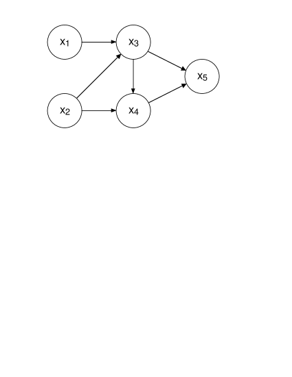
Figure 1: A Bayesian network. Evidence about any of the random variables influences the likelihood of the remaining random variables. In a straightforward terminology, the node at the tail of an arrow is a parent of the child node at the head of the arrow, e.g. $X_{4}$ is a parent of $X_{5}$ and a child of both $X_{2}$ and $X_{3}$. From the structure of the graph, we can see the conditional independence relations in the probabilistic model. For example, $X_{5}$ is independent of $X_{1}$ and $X_{2}$ given $X_{3}$ and $X_{4}$.

Bayesian networks have two properties that we will find very useful, both of which stem from the dependence relations shown by the graph structure. First, the value of a node $X$ is not dependent upon all of the other graph nodes. Rather, it depends only on a subset of the nodes, called a Markov blanket of $X$, that separates node $X$ from all the other nodes in the graph. The Markov blanket of interest to us is readily determined from the graph structure. It is comprised of the union of the direct parents of $X$, the direct successors of $X$, and all direct parents of the direct successors of $X$. Second, the joint probability over the random variables is decomposable as

$$P(x_{1},x_{2},\ldots,x_{n})=\prod_{\mu=1}^{n}P(x_{\mu}\!\mid\!\mathrm{Pa}(x_{\mu}))\enspace,$$ (1)

where $\mathrm{Pa}(x_{\mu})$ denotes the (possibly empty) set of direct-parent nodes of $X_{\mu}$. This decomposition comes about from repeated application of Bayes’ rule and from the structure of the graph.

3 Neural Network Model

We will develop neural networks from the set of marginal distributions $\left\{\rho(x_{\mu};t)\right\}$ so as to best match a desired probabilistic model $\rho(x_{1},x_{2},\ldots,x_{D})$ over the set of random variables, which are organized as a Bayesian network. One or more of the variables $x_{\mu}$ must be specified as evidence in the Bayesian network. To facilitate the development of general update rules, we do not distinguish between evidence and non-evidence nodes in our notation.

Our general approach will be to minimize the difference between a probabilistic model $\rho(x_{1},x_{2},\ldots,x_{D})$ and an estimate of the probabilistic model $\hat{\rho}(x_{1},x_{2},\ldots,x_{D})$. For the estimate, we utilize

$$\hat{\rho}(x_{1},x_{2},\ldots,x_{D})=\prod_{\alpha}\rho(x_{\alpha};t)\enspace.$$ (2)

This is a so-called naive estimate, wherein the random variables are assumed to be independent. We will place further constraints on the probabilistic model and representation to produce neural networks with the desired dynamics.

The first assumption we make is that the populations of neurons only need to accurately encode the mean values of the random variables, rather than the complete densities. We take the firing rates of the neurons representing a given random variable $X_{\alpha}$ to be functions of the mean value $\bar{x}_{\alpha}$(t)

$$a^{\alpha}_{i}(t)=g\left(A^{\alpha}_{i}\bar{x}_{\alpha}(t)+B^{\alpha}_{i}\right)\enspace,$$ (3)

where $A^{\alpha}_{i}$ and $B^{\alpha}_{i}$ are parameters describing the response properties of neuron $i$ of the population representing random variable $X_{\alpha}$. The activation function $g$ is in general nonlinear; in this work, we take $g$ to be the logistic function,

$$g\left(x\right)=\frac{1}{1+\exp\left(-x\right)}\enspace.$$ (4)

We use a set of neural response function (Fig. 2) similar to ones from work on population-temporal coding that supported manipulation of mean values [15, 16]. We can make use of Eq. 3 to directly encode mean values into neural activation states, providing a means to specify the value of the evidence nodes in the NBN.

Figure 2: The mean values of the random variables are encoded into the firing rates of populations of neurons. A population of twenty neurons with sigmoidal responses is associated with each random variable. The neuronal responses $a^{\alpha}_{i}$ are fully determined by a single input $\xi$, which we interpret as the mean value of a density. The form of the neuronal transfer functions can be altered without affecting the general result presented in this work.

Using Eq. 3, we derive an update rule describing the neuronal dynamics, obtaining (to first order in $\tau$)

$$a^{\alpha}_{i}(t+\tau)=g\left(A^{\alpha}_{i}\bar{x}_{\alpha}(t)+\tau A^{\alpha}_{i}\frac{d\bar{x}_{\alpha}(t)}{dt}+B^{\alpha}_{i}\right)\enspace.$$ (5)

Thus, if we can determine how $\bar{x}_{\alpha}$ changes with time, we can directly determine how the neural activation states change with time.

The mean value $\bar{x}_{\alpha}(t)$ can be determined from the firing rates as the expectation value of the random variable $X_{\alpha}$ with respect to a density $\rho(x_{\alpha};t)$ represented in terms of some decoding functions $\left\{\phi^{\alpha}_{i}\left(x_{\alpha}\right)\right\}$ The density is recovered using the relation

$$\rho(x_{\alpha};t)=\sum_{i}a^{\alpha}_{i}\phi^{\alpha}_{i}\left(x_{\alpha}\right)\enspace.$$ (6)

The decoding functions are constructed so as to minimize the difference between the assumed and reconstructed densities (discussed in detail in [17]).

With representations as given in Eq. 6, we have

$$\bar{x}_{\alpha}(t) =\int x_{\alpha}\rho\left(x_{\alpha};t\right)\,dx_{\alpha}$$

$$=\sum_{i}a^{\alpha}_{i}(t)\bar{x}^{\alpha}_{i}\enspace,$$ (7)

where we have defined

$$\bar{x}^{\alpha}_{i}=\int x_{\alpha}\phi^{\alpha}_{i}\left(x_{\alpha}\right)\,dx_{\mu}\enspace.$$ (8)

Although we used the decoding functions $\phi^{\alpha}_{i}\left(x_{\alpha}\right)$ to calculate the parameters $\bar{x}^{\alpha}_{i}$, they can in practice be found directly so that the relations in Eqs. 3 and 7 are mutually consistent.

We take the densities $\rho(x_{\alpha};t)$ to be normally distributed with the form $\rho(x_{\alpha};t)\equiv\rho(x_{\alpha};\bar{x}_{\alpha}(t))=N(x_{\alpha};\bar{x}_{\alpha}(t),\sigma_{x_{\alpha}}^{2})$. Intuitively, we might expect that the variance $\sigma_{x_{\alpha}}^{2}$ should be small so that the mean value is coded precisely, but we will see that the variances have no significance in the resulting neural networks.

The second assumption we make is that interactions between the nodes are linear:

$$x_{\beta}=\sum_{\alpha}K_{\beta\alpha}x_{\alpha}\enspace.$$ (9)

Utilizing the causality relations given by the Bayesian network, we require that $K_{\beta\alpha}\neq 0$ only if $X_{\beta}$ is a child node of $X_{\alpha}$ in the network graph. To represent the linear interactions as a probabilistic model, we take the normal distributions $\rho(x_{\beta}\!\mid\!\mathrm{Pa}(x_{\beta}))=N(x_{\beta};\sum_{\alpha}K_{\beta\alpha}x_{\alpha},\sigma_{\beta}^{2})$ for the conditional probabilities.

For nodes in the Bayesian network which have no parents, the conditional probability $\rho(x_{\beta}\!\mid\!\mathrm{Pa}(x_{\beta}))$ is just the prior probability distribution $\rho(x_{\beta})$. We utilize the same rule to define the prior probabilities as to define the conditional probabilities. For parentless nodes, the prior is thus normally distributed with zero mean, $\rho(x_{\beta})=N(x_{\beta};0,\sigma_{\beta}^{2})$.

We use the relative entropy [18] as a measure of the “distance” between the joint distribution describing the probabilistic model $\rho(x_{1},x_{2},\ldots,x_{D})$ and the density estimated from the neural network $\hat{\rho}(x_{1},x_{2},\ldots,x_{D})$. Thus, we minimize

$$E=-\int\hat{\rho}(x_{1},x_{2},\ldots,x_{D})\log\left(\frac{\rho(x_{1},x_{2},\ldots,x_{D})}{\hat{\rho}(x_{1},x_{2},\ldots,x_{D})}\right)\,dx_{1}dx_{2}\cdots dx_{D}$$ (10)

with respect to the mean values $\bar{x}_{\alpha}$. By making use of the gradient descent prescription

$$\frac{d\bar{x}_{\gamma}}{dt}=-\eta\frac{\partial E}{\partial\bar{x}_{\gamma}}$$ (11)

and the decomposition property for Bayesian networks given by Eq. 1, we obtain the update rule for the mean values,

$$\frac{d\bar{x}_{\gamma}}{dt}=\frac{\eta}{\sigma_{\gamma}^{2}}\left(\sum_{\beta}K_{\gamma\beta}\bar{x}_{\beta}-\bar{x}_{\gamma}\right)-\eta\sum_{\beta}\frac{K_{\beta\gamma}}{\sigma_{\beta}^{2}}\left(\sum_{\alpha}K_{\beta\alpha}\bar{x}_{\alpha}-\bar{x}_{\beta}\right)\enspace.$$ (12)

Because the coupling parameters $K_{\alpha\beta}$ are nonzero only when $X_{\alpha}$ is a parent of $X_{\beta}$, generally only a subset of the mean values contributes to updating $\bar{x}_{\gamma}$ in Eq. 12. In terms of the Bayesian network graph structure, the only contributing values come from the parents of $X_{\gamma}$, the children of $X_{\gamma}$, and the parents of the children of $X_{\gamma}$; this is identical to the Markov blanket discussed in Section 2.

The update rule for the neural activities is obtained by combining Eqs. 5, 7 and 12, resulting in

$$a^{\gamma}_{i}(t+\tau)=g\left(\sum_{j}S^{\gamma}_{ij}a^{\gamma}_{j}(t)+B^{\gamma}_{i}+\eta\tau h^{\gamma}_{i}(t)\right)\enspace.$$ (13)

The quantity $\sum_{j}S^{\gamma}_{ij}a^{\gamma}_{j}(t)+B^{\gamma}_{i}$ serves to stabilize the activities of the neurons representing $\rho(x_{\gamma})$, while

$$h^{\gamma}_{i}(t)=\sum_{j}T^{\gamma}_{ij}a^{\gamma}_{j}(t)+\sum_{\beta}\sum_{j}\left(U^{\gamma\beta}_{ij}+V^{\beta\gamma}_{ij}\right)a^{\beta}_{j}(t)+\sum_{\alpha,\beta}\sum_{j}W^{\gamma\beta\alpha}_{ji}a^{\alpha}_{j}(t)$$ (14)

drives changes in $a^{\gamma}_{i}(t)$ based on the densities represented by other nodes of the Bayesian network. The synaptic weights of the neural network are

$$S^{\gamma}_{ij} =A^{\gamma}_{i}{}\bar{x}^{\gamma}_{j}\enspace,$$ (15)

$$T^{\gamma}_{ij} =-A^{\gamma}_{i}{\frac{1}{\sigma_{\gamma}^{2}}}\bar{x}^{\gamma}_{j}\enspace,$$ (16)

$$U^{\gamma\beta}_{ij} =A^{\gamma}_{i}{\frac{1}{\sigma_{\gamma}^{2}}K_{\gamma\beta}}\bar{x}^{\gamma}_{j}\enspace,$$ (17)

$$V^{\beta\gamma}_{ij} =-A^{\gamma}_{i}{\frac{1}{\sigma_{\beta}^{2}}K_{\beta\gamma}}\bar{x}^{\gamma}_{j}\enspace,$$ (18)

$$W^{\gamma\beta\alpha}_{ji} =A^{\gamma}_{i}{\frac{1}{\sigma_{\gamma}^{2}}K_{\gamma\beta}K_{\beta\alpha}}\bar{x}^{\gamma}_{j}$$ (19)

The foregoing provides an algorithm for generating and evaluating neural networks that process mean values of random variables. To summarize,

1. Establish independence relations between model variables. This may be accomplished by using a graph to organize the variables.

2. Specify the $K_{\alpha\beta}$ to quantify the relations between the variables.

3. Assign network inputs by encoding desired values into neural activities using Eq. 3.

4. Update other neural activities using the update rule in Eq. 13 and the supporting definitions in Eqs. 14 to xtract the expectation values of the variables from the neural activities using Eq. 7.

   4 Examples

   As a first example, we apply the algorithm to the Bayesian network shown in Fig. 1, with firing rate profiles as shown in Fig. 2. Specifying $x_{1}=1/2$ and $x_{2}=-1/2$ as evidence, we find an excellent match between the mean values calculated by the neural network and the directly calculated values for the remaining nodes (Table 1).

   Table 1: The mean values decoded from the neural network closely match the values directly calculated from the linear relations. The coefficients for the linear combinations were randomly selected, with values $K_{31}=-0.2163$, $K_{32}=-0.8328$, $K_{42}=0.0627$, $K_{43}=0.1438$, $K_{53}=-0.5732$, and $K_{54}=0.5955$.

   Node	Direct Calculation	Neural Network
   $X_{1}$	0.5000	0.5000
   $X_{2}$	-0.5000	-0.5000
   $X_{3}$	0.3083	0.3084
   $X_{4}$	0.0130	0.0128
   $X_{5}$	-0.1690	-0.1689

   We next focus on some simpler Bayesian networks to highlight certain properties of the resulting neural networks (which will again utilize the firing rate profiles shown in Fig. 2). In Fig. 3, we present two Bayesian networks that relate three random variables in different ways. The connection strengths are all taken to be unity in each graph, so that $K_{21}=K_{23}=K_{12}=K_{13}=1$.

   With the connection strengths so chosen, the two Bayesian networks have straightforward interpretations. For the graph shown in Fig. 3, $X_{2}$ represents the sum of $X_{1}$ and $X_{3}$, while, for the graph shown in Fig. 3, $X_{2}$ provides a value which is duplicated in $X_{1}$ and $X_{3}$. The different graph structures yield different neural networks; in particular, nodes $X_{1}$ and $X_{3}$ have direct synaptic connections in the neural network based on the graph in Fig. 3, but no such direct weights exist in a second network based on Fig. 3. Thus, specifying $x_{1}=-1/4$ and $x_{2}=1/4$ for the first network produces the expected result $\bar{x}_{3}=-0.5000$, but specifying $x_{2}=1/4$ in the second network produces $\bar{x}_{3}=0.2500$ regardless of the value (if any) assigned to $x_{1}$.

   

   

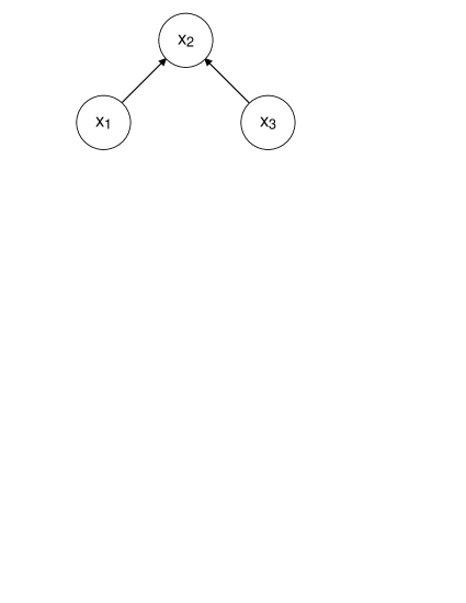
   Figure 3: Simpler Bayesian networks. Although the underlying undirected graph structure is identical for these two networks, the direction of the causality relationships between the variables are reversed. The neural networks arising from the Bayesian networks thus have different properties.

   To further illustrate the neural network properties, we use the graph shown in Fig. 3 to process inconsistent evidence. Nodes $X_{1}$ and $X_{3}$ should copy the value in node $X_{2}$, but we can specify any values we like as network inputs. For example, when we assign $x_{1}=-1/4$ and $x_{3}=1/2$, the neural network yields $\bar{x}_{2}=0.1250$ for the remaining value. This is a typical and reasonable result, matching the least-squares solution to the inconsistent problem.

   5 Conclusion

   We have introduced a class of neural networks that consistently mix multiple sources of evidence. The networks are based on probabilistic models, represented in the graphical form of Bayesian networks, and function based on traditional neural network dynamics (i.e., a weighted sum of neural activation values passed through a nonlinear activation function). We constructed the networks by restricting the represented probabilistic models by introducing two auxiliary assumptions.

   First, we assumed that only the mean values of the random variables need to be accurately represented, with higher order moments of the distribution being unimportant. We introduced neural representations of relevant probability density functions consistent with this assumption. Second, we assumed that the random variables of the probabilistic model are linearly related to one another, and chose appropriate conditional probabilities to implement these linear relationships.

   Using the representations suggested by our auxiliary assumptions, we derived a set of update rules by minimizing the relative entropy of an assumed density with respect to the density decoded from the neural network. In a straightforward fashion, the optimization procedure yields neural weights and dynamics that implement specified probabilistic relations, without the need for a training process.

   The neural networks investigated in this work captures many of the properties of both Bayesian networks and traditional neural network models. In particular, multiple sources of evidence are consistently pooled based on local update rules, providing a distributed version of a probabilistic model.

   Acknowledments

   This work was supported by the U.S. National Science Foundation, by the Portuguese Fundação para a Ciência e a Technologia (FCT) under Bolsa SFRH/BPD/9417/2002, and by the Austrian Science Fund (FWF) under project P21450. JWC also acknowledges support received from the Fundação Luso-Americana para o Desenvolvimento (FLAD) and from the FCT for his participation in Madeira Math Encounters XXIII at the University of Madiera, where portions of the work were conducted.

References

- Anderson and Abrahams [1987] C. H. Anderson, E. Abrahams, The Bayes connection, in: Proceedings of the IEEE First International Conference on Neural Networks, volume III, IEEE, SOS Print, San Diego, CA, 1987, pp. 105–112.
- Zemel et al. [1998] R. S. Zemel, P. Dayan, A. Pouget, Probabilistic interpretation of population codes, Neural Comput. 10 (1998) 403–30.
- Zemel [1999] R. S. Zemel, Cortical belief networks, in: R. Hecht-Neilsen (Ed.), Theories of Cortical Processing, Springer-Verlag, Berlin, 1999.
- Zemel and Dayan [1999] R. S. Zemel, P. Dayan, Distributional population codes and multiple motion models, in: M. S. Kearns, S. A. Solla, D. A. Cohn (Eds.), Advances in Neural Information Processing Systems 11, MIT Press, Cambridge, MA, 1999.
- Yang and Zemel [2000] Z. Yang, R. S. Zemel, Managing uncertainty in cue combination, in: S. A. Solla, K. R. Leen, T. K. and. Müller (Eds.), Advances in Neural Information Processing Systems 12, MIT Press, Cambridge, MA, 2000.
- Haykin [1999] S. Haykin, Neural Networks: A Comprehensive Foundation, Prentice Hall, Upper Saddle River, NJ, second edition, 1999.
- Hinton and Sejnowski [1986] G. E. Hinton, T. J. Sejnowski, Learning and relearning in Boltzmann machines, in: D. E. Rumelhart, J. L. McClelland, et al. (Eds.), Parallel Distributed Processing: Explorations in Microstructure of Cognition, MIT Press, Cambridge, MA, 1986, pp. 282–317.
- Neal [1992] R. M. Neal, Connectionist learning of belief networks, Artificial Intelligence 56 (1992) 71–113.
- Dayan and Hinton [1996] P. Dayan, G. E. Hinton, Varieties of Helmholtz machines, Neural Networks 26 (1996) 1385–1403.
- Pearl [1988] J. Pearl, Probabilistic Reasoning in Intelligent Systems: Networks of Plausible Inference, Morgan Kaufmann, San Mateo, CA, 1988.
- Smyth et al. [1997] P. Smyth, D. Heckerman, M. I. Jordan, Probabilistic independence networks for hidden Markov probability models, Neural Comput. 9 (1997) 227–69.
- George and Hawkins [2005] D. George, J. Hawkins, A hierarchical bayesian model of invariant pattern recognition in the visual cortex, volume 3, pp. 1812–1817.
- Barber et al. [2003a] M. J. Barber, J. W. Clark, C. H. Anderson, Neural representation of probabilistic information, Neural Comp. 15 (2003a) 1843–1864.
- Barber et al. [2003b] M. J. Barber, J. W. Clark, C. H. Anderson, Generating neural circuits that implement probabilistic reasoning, Physical Review E (Statistical, Nonlinear, and Soft Matter Physics) 68 (2003b) 041912.
- Eliasmith and Anderson [1999] C. Eliasmith, C. H. Anderson, Developing and applying a toolkit from a general neurocomputational framework, Neurocomputing 26 (1999) 1013–1018.
- Eliasmith and Anderson [2002] C. Eliasmith, C. H. Anderson, Neural Engineering: The Principles of Neurobiological Simulation, MIT Press, 2002.
- Barber et al. [2003] M. J. Barber, J. W. Clark, C. H. Anderson, Neural representation of probabilisitic information, Neural Comp. 15 (2003) 1843–1864.
- Papoulis [1991] A. Papoulis, Probability, Random Variables, and Stochastic Processes, McGraw-Hill, Inc., New York, NY, third edition, 1991.