Magnetic field induced non-Gaussian fluctuations in macroscopic equilibrium systems

Abstract

We calculate the magnetic-field dependent nonlinear conductance and noise in a two-dimensional macroscopic inhomogeneous system. If the system does not possess a specific symmetry, the magnetic field induces a nonzero third cumulant of the current even at equilibrium. This cumulant is related to the first and second voltage derivatives of the spectral density and average current in the same way as for mesoscopic quantum-coherent systems, but these quantities may be much larger. The system provides a robust test of a non-equilibrium fluctuation relation.

It is commonly believed that equilibrium fluctuations in macroscopic systems are Gaussian Landau . If their correlation length $l_{c}$ is much smaller than all the dimensions of the sample $L$, this is a direct consequence of the central limit theorem, which says that the sum of a large number of random variables will have approximately normal distribution. This is why higher cumulants of current are usually calculated and measured for mesoscopic systems, whose size is smaller than $l_{c}$. Typically, $l_{c}$ is the inelastic scattering length and if $L<l_{c}$, the conductor behaves as a single quantum scatterer. In a macroscopic system, higher cumulants are usually much smaller than the second one. However some fluctuations do not exponentially decay with distance and therefore do not have a definite correlation length. For example, fluctuations of charge density in two-dimensional conductors are screened according to a power law. If they are nonlinearly coupled to the current, this may result in a non-Gaussian noise even in an equilibrium macroscopic system. Below we propose a model of such noise. Moreover, the nonzero equilibrium third cumulant of current in it obeys the fluctuation relations recently derived for mesoscopic systems.

The last several years saw an increase of interest to fluctuation–dissipation relations that apply beyond the linear transport regime Tobiska05 ; Andrieux . Based on the symmetry properties of the cumulant generating function in the full counting statistics of transferred charge Levitov93 , universal relations between cumulants of current of different order and their voltage derivatives were obtained.

Recent studies Forster08 ; Saito08 ; Sanchez09 showed that the fluctuation relations hold even in a magnetic field that breaks the microscopic reversibility. In particular, they link the contribution to the mean current proportional to magnetic field and quadratic in voltage $\Delta I\propto V^{2}H$ to a noise contribution proportional to the temperature, magnetic field, and voltage $\Delta S\propto THV$, and to the third cumulant of equilibrium current fluctuations $C_{0}$. Consequently, this cumulant is an odd function of the magnetic field. However the relations obtained in Forster08 and Saito08 differ. Förster and Büttiker Forster08 obtained that $C_{0}=3T\,[\partial\Delta S/\partial V-T\,\partial^{2}\Delta I/\partial V^{2}]$, whereas Saito and Utsumi Saito08 obtained a stronger condition $C_{0}=2T\,\partial\Delta S/\partial V=6T^{2}\,\partial^{2}\Delta I/\partial V^{2}$ valid for a more restricted class of systems. The weaker condition permits magnetic field asymmetric conductance and noise even if the third cumulant of the equilibrium noise vanishes.

The nonlinear contributions to the average current $\Delta I\propto V^{2}H$ were calculated for a number of mesoscopic systems. Sanchez and Polianski and one of the authors Sanchez04 ; Polianski06 investigated a quantum Hall bar with an antidot and a chaotic cavity connected to quantum point contacts. Spivak and Zuyzin Spivak04 calculated this contribution for a mesoscopic diffusive system, whereas Andreev and Glazman Andreev06 studied it for a semiclassical ballistic contact with an asymmetric obstacle. This contribution was observed in several experiments Zumbuhl06 ; Leturcq06 ; Angers07 ; Brandenstein09 . A qualitative relation between the magnetic field asymmetric current $\Delta I$ and the voltage derivative of the noise $\Delta S$ was established in a pioneering experiment for an Aharonov–Bohm interferometer Nakamura10 .

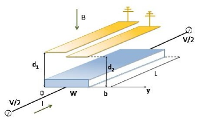
Figure 1: A sketch of a diffusive conductor with an asymmetric gate. Its I-V-characteristics, noise and the third cumulant of equilibrium noise are magnetic-field asymmetric. Gap heights $d_{1}$ and $d_{2}$ correspond to $\alpha_{1}$ and $\alpha_{2}$ in Eq. (17).

The fluctuation relations in a magnetic field Forster08 ; Saito08 were derived for mesoscopic systems assuming conservation of the electron energy. Therefore it is of interest to test them for a macroscopic system with a strong energy dissipation by explicitly calculating the relevant quantities. Here we consider a system that can be made arbitrarily large and yet exhibits non-Gaussian noise due to long-range charge fluctuations. We use it to test the nonlinear fluctuation–dissipation relations in a magnetic field. Because of the macroscopic nature of the system, the quantities in hand may reach much higher values than in mesoscopic conductors and are more easy to measure.

Model. To perform our test, we need a macroscopic conductor that possesses a nonlinear conductivity and lacks symmetry in the direction transverse to the current. The system of our choice (shown in Fig. 1) is a conducting slab with a thickness much smaller than the charge screening length and two perfect electrodes. The slab is threaded by a magnetic field normal to its surface, and a grounded gate is mounted on top of it. The narrow gap of height $d_{g}$ between the slab and the gate and the 2D conductivity of the slab $\sigma_{0}$ are spatially nonuniform. We also assume a diffusive transport and a strong energy relaxation so that the local distribution of electrons is in equilibrium and the local conductivity is determined solely by the electron sheet density $n_{s}$. The conductor and the gate form together a plane capacitor so that the electron density in the slab is related to the local potential $\varphi({\bf r})$ by $e(n_{s}-n_{0})=\varepsilon_{d}\varphi/4\pi d_{g},$ where $n_{0}$ is the equilibrium electron density at $\varphi=0$ and $\varepsilon_{d}$ is the dielectric constant of the insulator in the gap. Therefore the local conductivity depends on the local potential, i. e.

$$\sigma({\bf r})=\sigma_{0}({\bf r})\,[1+\alpha({\bf r})\,\varphi({\bf r})],\qquad$$

$$\sigma_{0}=\frac{e^{2}n_{0}({\bf r})\tau_{tr}}{m},\quad\alpha({\bf r})=\frac{\varepsilon_{d}}{4\pi en_{0}({\bf r})\,d_{g}({\bf r})},$$ (1)

where $m$ is the electron mass and $\tau_{tr}$ is its coordinate- and energy-independent scattering time. The sensitivity of $\sigma({\bf r})$ to the potential leads to a current which is nonlinear in the applied voltage. If a current flows from one electrode to another in a magnetic field, it induces a Hall voltage across the conductor. If $\alpha({\bf r})$ is asymmetric in the direction transverse to the current, the different directions of current or magnetic field will result in different changes of conductivity and hence the antisymmetric component $\Delta I\propto V^{2}H$ should appear in the current.

In a magnetic field $H$, the local current density is

$${\bf j}=-\sigma_{0}\,(1+\hat{\beta})(1+\alpha\varphi)\,\nabla\varphi,\quad\hat{\beta}=\left(\begin{array}[]{rr}0&\beta\\ -\beta&0\\ \end{array}\right),$$ (4)

where the matrix $\hat{\beta}$ acts on the vector $\nabla\varphi$ and $\beta=eH/(mc)\,\tau_{tr}$ is proportional to $H$. The current density satisfies the continuity equation $\nabla\cdot{\bf j}=0\,.$ The boundary conditions at the left and right electrodes are $\left.\varphi({\bf r})\right|_{L}=V_{L}$ and $\left.\varphi({\bf r})\right|_{R}=V_{R}$, where $V_{R}-V_{L}=V$. The rest of the conductor boundary is impenetrable to the current. Without loss of generality, we assume that $\sigma_{0}$ smoothly turns to zero at the insulating boundary whereas ${\bf n}\cdot\nabla\varphi$ remains finite there.

Average current. We solve the continuity equation by expanding $\varphi$ and ${\bf j}$ in $\alpha$ and $\beta$ ,

$$\varphi=\varphi_{0}+\varphi_{\alpha}+\varphi_{\beta}+\varphi_{\alpha\beta},\quad{\bf j}={\bf j}_{0}+{\bf j}_{\alpha}+{\bf j}_{\beta}+{\bf j}_{\alpha\beta}.$$ (5)

In our derivation, we use an approach similar to that of Sukhorukov98 . The correction to the total current flowing through the conductor is conveniently expressed in terms of the characteristic potential $\psi$ of the left contact that obeys an equation ${\cal L}\psi\equiv\nabla\cdot(\sigma_{0}\nabla\psi)=0$ with boundary conditions $\left.\psi\right|_{L}=1$ and $\left.\psi\right|_{R}=0$ Buttiker93 so that $\varphi_{0}=V_{L}\,\psi+V_{R}\,(1-\psi)$. In the absence of a magnetic field, $\psi$ allows one to map the conductor on a purely one-dimensional system, where it plays the role of the longitudinal coordinate $x$. For vanishing $\alpha$ and magnetic field, the current through the conductor can be written in a form

$$I_{0}={V}\int d^{2}r\,\sigma_{0}\,(\nabla\psi)^{2}.$$ (6)

We obtain the first order nonlinear correction in $\alpha$ to the current by separating the component ${\bf j}_{\alpha}$ in Eq. (4) which takes the form of an integral

$$I_{\alpha}={V}\int d^{2}r\,\alpha\,\sigma_{0}\,\varphi_{0}\,(\nabla\psi)^{2}.$$ (7)

This quantity is proportional to the nonlinear correction to the local conductivity averaged over the conductor with a weigh factor $(\nabla\psi)^{2}$. It vanishes for a symmetric conductor if $V_{L}=-V_{R}$. The quadratic nonlinear conductance and the rectification effect were recently discussed in detail in Polianski07 .

The antisymmetric contribution to the current $I_{\alpha\beta}$ can be calculated by isolating the corresponding component in Eq. (4). We can present $\Delta I\equiv I_{\alpha\beta}$ in the form

$$\Delta I={V^{2}}\!\int d^{2}r\,\alpha\,\sigma_{0}\,(\nabla\psi)^{2}{\cal L}^{-1}\left[(\nabla\sigma_{0})\cdot\hat{\beta}\,\nabla\psi\right],$$ (8)

where ${\cal L}^{-1}$ is the inverse of differential operator ${\cal L}$ taken with zero boundary conditions. This component of the current results from the Hall voltage and the related correction to the conductivity. Note that in a magnetic field, the problem cannot be mapped onto a one-dimensional one. Therefore the operator ${\cal L}^{-1}$ cannot be eliminated from the right-hand side of Eq. (8) in contrast to Eq. (6) for $\delta I_{\alpha}$.

Noise. To find the spectral density of electric noise, i. e. the second cumulant of the current, we use the Langevin approach Kogan96 . To this end, we linearize Eq. (4) with respect to small fluctuations $\delta\varphi$ and $\delta{\bf j}$ and add a random extraneous current $\delta{\bf j}^{ext}$ to its right-hand side so that

$$\delta{\bf j}=-\sigma_{0}(1+\hat{\beta})[\nabla\delta\varphi+\alpha\nabla(\varphi\,\delta\varphi)]+\delta{\bf j}^{ext}.$$ (9)

We are interested in the low-frequency fluctuations for which the continuity equation $\nabla\cdot\delta{\bf j}=0$ holds. The fluctuations also obey the boundary conditions $\delta\varphi=0$ at the electrodes and ${\bf n}\,\delta{\bf j}=0$ at the rest of the boundary. The continuity equation results in a diffusion-type equation in $\delta\varphi$. Using the formal solution of this equation and Eq. (9), we express the fluctuation $\delta I$ in terms of $\delta{\bf j}^{ext}$. Then the product of two different realizations $\delta I$ has to be averaged using the correlation function of extraneous currents. We assume that because of a strong energy relaxation the local distribution of electrons is equilibrium for a given electric potential and therefore this correlation function is given by

$$\langle\delta j_{x,y}^{ext}({\bf r}_{1})\,\delta j_{x,y}^{ext}({\bf r}_{2})\rangle=2T\,\delta({\bf r}_{1}-{\bf r}_{2})\,$$

$$\times[1+\alpha\,\varphi({\bf r}_{1})]\,\sigma_{0}({\bf r}_{1}).$$ (10)

Extraneous currents $\delta j_{x}^{ext}$ and $\delta j_{y}^{ext}$ are uncorrelated because their correlation function is proportional Landau to $\sigma_{xy}(H)+\sigma_{yx}(H)=(\sigma_{0}\hat{\beta})_{12}+(\sigma_{0}\hat{\beta})_{21}=0$.

We solve Eq. (9) by expanding $\delta\varphi$ and $\delta{\bf j}$ in $\alpha$ and $\beta$ similarly to Eqs. (5). In the zero approximation, we obtain a formal expression for the current fluctuation $\delta I_{0}=\int d^{2}r\,(\nabla\psi)\cdot\delta{\bf j}^{ext},$ which leads to the spectral density of current of the form

$$S_{0}=2T\int d^{2}r\,\sigma_{0}\,(\nabla\psi)^{2}\equiv 2T\,\partial I_{0}/\partial V$$ (11)

that satisfies the usual Nyquist theorem.

The correction to the spectral density proportional to voltage equals

$$S_{\alpha}=2T\int d^{2}r\,\alpha\sigma_{0}\varphi_{0}\,(\nabla\psi)^{2}\equiv 2T\,\partial I_{\alpha}/\partial V.$$ (12)

The second part of this equation is exactly the relation established in Refs. Forster08 ; Saito08 for the quantities symmetrized with respect to the magnetic field.

The correction to the noise $S_{\alpha\beta}$ proportional to both voltage and magnetic field is determined by the components of the current fluctuation $\delta I_{0}$, $\delta I_{\alpha}$, and $\delta I_{\beta}$. Long but simple calculations lead to the expression for $\Delta S\equiv S_{\alpha\beta}$ of a form

$$\Delta S=6T\,{V}\int d^{2}r\,\alpha\sigma_{0}\,(\nabla\psi)^{2}\,{\cal L}^{-1}\left[(\nabla\sigma_{0})\cdot\hat{\beta}\,\nabla\psi\right],$$ (13)

hence the antisymmetric contribution to the noise satisfies the condition $\partial\Delta S/\partial V=3T\,\partial^{2}\Delta I/\partial V^{2}$ Saito08 . The presence of this contribution to the noise suggests that in a nonzero magnetic field, the minimum in the voltage dependence of noise Forster09 is shifted away from $V=0$.

Third cumulant. To calculate the equilibrium third cumulant of current, we use the semiclassical cascade approach Nagaev02 ; Pilgram03 ; Jordan04 . We assume that the conductor is diffusive and therefore the local random Langevin currents have a Gaussian distribution with zero third cumulant Nagaev02 . However these random currents induce fluctuations of the potential $\delta\varphi$, which may affect the correlator of Langevin currents at a different point by changing the local conductivity (1) that enters into Eq. (10). This results in an irreducible correlation between three observable currents. The third cumulant of current is

$$C=3\int d^{2}r\,\frac{\delta S}{\delta\varphi({\bf r})}\,\langle\delta\varphi({\bf r})\,\delta I\rangle,$$ (14)

where ${\delta S}/{\delta\varphi({\bf r})}$ is the functional derivative of the spectral density of the current $S$ with respect to the local potential $\varphi$ at point ${\bf r}$. As this derivative is proportional to $\alpha$, the correlator $\langle\delta\varphi({\bf r})\,\delta I\rangle$ should be calculated to the zero approximation in this parameter. In the required approximation, the sought-for correlator equals

$$\langle\delta\varphi({\bf r})\,\delta I\rangle=2T{\cal L}^{-1}\!\left[(\nabla\sigma_{0})\cdot\hat{\beta}\,\nabla\psi\right]$$ (15)

and vanishes in zero magnetic field. Thus ${\delta S}/{\delta\varphi({\bf r})}$ is needed only to the zero order in $\beta$ and therefore

$$C_{0}=12\,T^{2}\int d^{2}r\,\alpha\sigma_{0}\,(\nabla\psi)^{2}\,{\cal L}^{-1}\!\left[(\nabla\sigma_{0})\cdot\hat{\beta}\,\nabla\psi\right].$$ (16)

$C_{0}$ is proportional to $T^{2}$ and vanishes in zero magnetic field. Like the asymmetric part of $S$, it is proportional to the asymmetric part of the nonlinear conductance and satisfies the relation $C_{0}=6T^{2}\,\partial^{2}\Delta I/\partial V^{2}$ Saito08 . In the quantum-coherent approach Forster09 , the $T^{2}$ dependence of the third cumulant was explained with the energy dependence of electron transmission through the conductor. In semiclassics, it arises quite naturally because Eq. (16) actually involves a product of two correlators of thermal noise (10). At equilibrium and in the absence of magnetic field the local potential fluctuations do not contribute to the fluctuation of total current, and therefore $\delta\varphi$ and $\delta I$ are uncorrelated. It is the magnetic field that introduces a correlation between them as the fluctuation $\delta I$ immediately leads to a fluctuation of the Hall voltage in the transverse direction. To exhibit a nonvanishing third cumulant of current, the system must possess a certain asymmetry so that the fluctuation of the Hall voltage is not averaged out upon integration over its area.

Example. Consider a specific example of a rectangular conductor with $\sigma_{0}=$const and dimensions $0<x<L$ and $0<y<W$ with the current flowing in the $x$ direction. Assume that the gate above the conductor is split in the direction transverse to the current so that $\alpha(y)=\alpha_{1}\Theta(W/2-y)+\alpha_{2}\Theta(y-W/2)$, where $\Theta(y)$ is the Heaviside step function. Calculations by means of Eq. (8) give

$$\Delta I=\frac{4}{\pi^{4}}\,\beta\,\sigma_{0}\,(\alpha_{1}-\alpha_{2})\,V^{2}$$

$$\times\sum_{n=0}^{\infty}\frac{1-(-1)^{n}}{n^{4}}\left[1-\frac{1}{\cosh(n\pi W/2L)}\right].$$ (17)

For long and narrow conductors with $W\ll L$ this expression reduces to $(1/8)\,\beta\,\sigma_{0}\,(\alpha_{1}-\alpha_{2})\,V^{2}\,(W/L)^{2}$. In the opposite limit of short and wide contacts $L\ll W$ it saturates as a function of $W/L$ and tends to $(1/12)\,\beta\,\sigma_{0}\,(\alpha_{1}-\alpha_{2})\,V^{2}$. The $\Delta I(W/L)$ curve is shown in Fig. 2. For a square conductor, the $\Delta I/I_{0}$ ratio does not depend on its size and appears to be much larger than for a mesoscopic system. For a quantum-coherent mesoscopic system of size $d$ one can use an estimate $\Delta I_{Q}\sim e(eH/mc)(eV\tau_{d}/h)^{2}$, where $\tau_{d}$ is the dwell time of an electron in the system and $h$ is the Planck’s constant Sanchez04 ; Spivak04 . As the maximum $H$ and $V$ in this equation can be evaluated from the conditions $Hd^{2}\sim\Phi_{0}\equiv hc/e$ and $eV\tau_{d}\sim h$, one obtains the maximum value of the asymmetric current of the order of $\Delta I_{Q}\sim e(\varepsilon_{F}/h)(\lambda_{F}/d)^{2}$, where $\varepsilon_{F}$ is the Fermi energy and $\lambda_{F}$ is the Fermi wavelength. An estimate of Eq. (17) for a degenerate two-dimensional electron gas made on the assumption that $\alpha V\sim 1$ and $\beta\sim 1$ gives us $\Delta I_{M}\sim e(\varepsilon_{F}/h)(l_{tr}d_{g}/a_{B}\lambda_{F})$, where $l_{tr}=v_{F}\tau_{tr}$ and $a_{B}=\varepsilon_{d}\hbar^{2}/me^{2}$ is the Bohr radius of an electron in the conductor. The ratio of these quantities $\Delta I_{Q}/\Delta I_{M}\sim\lambda_{F}^{3}a_{B}/d^{2}d_{g}l_{tr}$ is much smaller than unity.

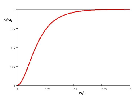
Figure 2: The ratio of the term $\Delta I$ for a rectangular conductor to its saturation value $\Delta I_{S}=(1/12)\,\beta\,\sigma_{0}\,(\alpha_{1}-\alpha_{2})\,V^{2}$ as a function of its width-to-length ratio.

Discussion. Equations (13) and (16) suggest that the system exhibits a component of noise $\Delta S\propto VH$ and an equilibrium third cumulant of current $C_{0}\sim T^{2}\beta\sigma_{0}(\alpha_{1}-\alpha_{2})$. The ratio of $C_{0}$ to the conductance is independent of the size of the square conductor precisely as for a mesoscopic system. As the third cumulant is insensitive to inelastic scattering, it can be made much larger than in mesoscopic systems by increasing temperature.

In summary, we have made predictions for the non-linear conductance, the voltage dependence of noise and the third cumulant in a macroscopic system with a strong energy dissipation. Long-range fluctuations of charge along with nonlinearity, macroscopic inhomogeneity and the magnetic field lead in particular to a nonzero third cumulant of current at equilibrium. This cumulant is proportional to the magnetic-field-asymmetric nonlinear conductance and voltage-dependent noise and satisfies the stronger form of the two fluctuation relations derived for quantum-coherent transport. This suggests that quantum coherence or energy conservation are not necessary for these relations to hold and they may be considered as universal. The macroscopic size of the third cumulant makes its measurement possible and thus could provide an experimental confirmation of the first non-trivial fluctuation relation.

Acknowledgments. This work is supported by the Swiss NSF, the center for excellence MaNEP and the European ITN NanoCTM.

References

- (1) L.D. Landau, E.M. Lifshitz, Statistical Physics, Part 1. Vol. 5 (3rd ed.) (Butterworth-Heinemann, 1980).
- (2) J. Tobiska and Yu. V. Nazarov, Phys. Rev. B 72, 235328 (2005).
- (3) D. Andrieux et al., New J. Phys. 043014 (2009).
- (4) L. S. Levitov and G. B. Lesovik, JETP Lett. 58, 230 (1993).
- (5) H. Förster and M. Büttiker, Phys. Rev. Lett. 101, 136805 (2008).
- (6) K. Saito and Y. Utsumi, Phys. Rev. B 78, 115429 (2008).
- (7) D. Sanchez, Phys. Rev. B79, 045305 (2009.)
- (8) D. Sanchez and M. Büttiker, Phys. Rev. Lett. 93, 106802 (2004).
- (9) M. L. Polianski and M. Büttiker, Phys. Rev. Lett. 96, 156804 (2006).
- (10) B. Spivak and A. Zyuzin, Phys. Rev. Lett. 93, 226801 (2004).
- (11) A. V. Andreev and L. I. Glazman, Phys. Rev. Lett. 97, 266806 (2006).
- (12) D. M. Zumbuhl, C. M. Marcus, M. P. Hanson, and A. C. Gossard, Phys. Rev. Lett. 96, 206802 (2006)
- (13) R. Leturcq et al., Phys. Rev. Lett. 96, 126801 (2006)
- (14) L. Angers et al., Phys. Rev. B 75, 115309 (2007)
- (15) B. Brandenstein-Köth, L. Worschech, and A. Forchel, Appl. Phys. Lett. 95, 062106 (2009)
- (16) S. Nakamura et al., Phys. Rev. Lett. 104, 080602 (2010)
- (17) E. V. Sukhorukov and D. Loss, Phys. Rev. B 59, 13054 (1999).
- (18) M. Büttiker, J. Phys.: Condens. Matter 5, 9361 (1993).
- (19) M. L. Polianski and M. Büttiker, Phys. Rev. B 76, 205308 (2007)
- (20) Sh. M. Kogan, Electronic noise and fluctuations in solids (Cambridge University Press, 1996)
- (21) H. Förster and M. Büttiker, arXiv:0903.1431
- (22) K. E. Nagaev, Phys. Rev. B 66, 075334 (2002).
- (23) S. Pilgram, A. N. Jordan, E. V. Sukhorukov, and M. Büttiker, Phys. Rev. Lett. 90, 206801 (2003).
- (24) A. N. Jordan, E. V. Sukhorukov, and S. Pilgram, J. Math. Phys. 45, 4386 (2004).