Spline approximation of a random process with singularity

Abstract

Let a continuous random process $X$ defined on $[0,1]$ be $(m+\beta)$-smooth, $0\leq m$, $0<\beta\leq 1$, in quadratic mean for all $t>0$ and have an isolated singularity point at $t=0$. In addition, let $X$ be locally like a $m$-fold integrated $\beta$-fractional Brownian motion for all nonsingular points. We consider approximation of $X$ by piecewise Hermite interpolation splines with $n$ free knots (i.e., a sampling design, a mesh). The approximation performance is measured by mean errors (e.g., integrated or maximal quadratic mean errors). We construct a sequence of sampling designs with asymptotic approximation rate $n^{-(m+\beta)}$ for the whole interval.

Keywords: Approximation, random process, sampling design, Hermite splines

1 Introduction

Let a random process $X(t),\,t\in[0,1]$, with finite second moment be observed in $n$ points and have different quadratic mean (q.m.) smoothness at $t=0$ (i.e., an isolated singularity). We consider piecewise polynomial approximation of $X$, combining two different Hermite interpolation splines for the interval adjacent to the singularity point and for the remaining part (i.e., a composite Hermite interpolation spline). A sequence of sampling designs (i.e., meshes) is constructed to improve the asymptotic approximation performance (e.g., integrated or maximal q.m. errors) eliminating the effect of the singularity point. The proposed technique can be applied also to random processes with a finite number of isolated singularity points. In principle, the main idea is well-known for nonlinear approximation of deterministic functions (see, e.g., de Boor, 1973, DeVore, 1998, and references therein). We use a finer mesh where the target function is singular and a coarser mesh where it is smooth. The primary question remains however: how to measure this smoothness for random functions in order to obtain definitive results.

More precisely, let $l$-th derivative of $X$ satisfy an $\alpha$-Hölder condition $0\leq l,0<\alpha\leq 1$, for $[0,1]$. It is known that the approximation rate $n^{-(l+\alpha)}$ is optimal in a certain sense for such class of processes and Hermite splines (see, e.g., Buslaev and Seleznjev, 1999, Seleznjev, 2000). Let, additionally, $X$ have a continuous $m$-th derivative satisfying a local stationarity condition, Berman (1974), with parameter $\beta$, and $0\leq m,0<\beta<1,l+\alpha\leq m+\beta$, for all points $t\in(0,1]$. We approximate $X$ by a corresponding composite Hermite interpolation spline and set up a sequence of sampling designs attaining the asymptotic approximation rate $n^{-(m+\beta)}$ for the whole interval $[0,1]$.

The nonlinear approximation results obtained in this paper are related to various problems in signal processing (e.g., optimization of compressing digitized signals, see, e.g., Cohen and D’Ales, 1997, Cohen et al., 2002), in numerical analysis of random functions (see, e.g., Benhenni and Cambanis, 1992, Kon and Plaskota, 2005, Creutzig and Lifshits, 2006, Creutzig et al., 2007), in simulation studies with controlled accuracy for functionals on realizations of random processes (see, e.g., Eplett, 1986, Abramowicz and Seleznjev, 2008). Hermite spline interpolation for continuous and smooth random functions is studied in Seleznjev (1996, 2000), and Huesler et al. (2003). Ritter (2000) contains a very detailed survey of various random function approximation problems.

The paper is organized as follows. First we introduce a basic notation. In Section 2, we consider composite spline interpolation for certain Hölder type classes of random processes, which behave locally like $m$-fold integrated fractional Brownian motion for all intervals $[a,b]\subset(0,1]$ and construct sequences of sampling designs with asymptotically optimal approximation rate. In the second part of the section, the approximation of more general Hölder’s classes of random functions and the accuracy for the corresponding composite Hermite spline approximation are studied. Sections 3 and 4 contain the results of numerical experiments and the proofs of the statements from Section 2, respectively.

1.1 Basic notation

Let $X=X(t),\,t\in[0,1]$, be defined on a probability space $(\Omega,\mathscr{F},P)$. Assume that for every $t$, the random variable $X(t)$ lies in the normed linear space $L^{2}(\Omega)=L^{2}(\Omega,\mathscr{F},P)$ of random variables with finite second moments and identified equivalent elements with respect to $P$. We set $||\,Z\,||:=(\mbox{E}\,Z^{2})^{1/2}$ for all $Z\in L^{2}(\Omega)$. Let ${\cal C}^{m}([0,1])$ denote the space of random processes with continuous q.m. derivatives up to order $m\geq 0$, and $C^{m}([0,1])$ be the corresponding space of non-random functions. Let ${\cal P}_{k}([0,1])$ be the space of stochastic polynomials of order $k\geq 0$. We define the norm for any $X\in{\cal C}^{m}([0,1])$ by setting

$$||\,X\,||_{p}:=\left(\int^{1}_{0}||\,X(t)\,||^{p}dt\right)^{1/p},\quad 1\leq p<\infty,$$

and $||\,X\,||_{\infty}:=\max_{[0,1]}||\,X(t)\,||$ for $p=\infty$. Henceforth, we use the convention, that if $p=\infty$, then $1/p=0$. Denote by $f(t)\asymp g(t)$ as $t\to a$ the weak equivalence property, i.e., $C_{1}~{}g(t)~{}\leq~{}f(t)~{}\leq~{}C_{2}~{}g(t)$ for some positive $C_{1},C_{2},b$ and for all $t\in(a,b]$ and similarly for $a_{n}\asymp b_{n}$ as $n\to\infty$.

Let $X$ be sampled at the distinct design points $T_{n}:=(t_{0},t_{1},\ldots,t_{n})$ (also referred to as knots), and the set of all $(n+1)$-point designs be denoted by $D_{n}:=\{T_{n}:0=t_{0}<t_{1}<\cdots<t_{n}=1\}$. We suppress the argument $n$ for the design points $t_{k}=t_{k}(n)$ from $T_{n}$, $\;k=0,\ldots,n$, when doing so causes no confusion. Recall that, for any $f\in C^{m}([0,1]),\;m\geq 0$, the piecewise Hermite polynomial $H_{k}(t)=H_{k}(f,T_{n})(t)$, of degree $k=2r+1$, $0\leq r\leq m$, is the unique solution of the interpolation problem $H_{k}^{(j)}(t_{i})=f^{(j)}(t_{i})$, where $i=0,\ldots,n$, $j=0,\ldots,r$. Analogously, we suppose that for $X\in{\cal C}^{m}([0,1])$, the process and its first $r\leq m$ derivatives can be sampled, and write $H_{k}(X,T_{n})$ with $k=2r+1\leq 2m+1$ to denote a corresponding stochastic Hermite spline. Define ${H}_{q,k}(X,T_{n}),\,q\leq k$, to be a composite Hermite spline

$${H}_{q,k}(X,T_{n}):=\left\{\begin{array}[]{rl}H_{q}(X,T_{n})(t),&t\in[0,t_{1}]\\ H_{k}(X,T_{n})(t),&t\in[t_{1},1]\end{array}\right..$$

To formulate the asymptotic results, we introduce a quasi regular sequence (qRS) of sampling designs $\{T_{n}=T_{n}(h)\}$ generated by a positive density function $h(t),\,t\in(0,1]$, via

$$\int_{0}^{t_{i}}h(t)\;dt=i/n,\quad i=1,\ldots,n,\quad\int_{0}^{1}h(t)dt=1.$$ (1)

Henceforth we assume that $h(t)$ is continuous for $t\in(0,1]$ and if $h(t)$ is unbounded in $t=0$, then $h(t)\to+\infty$ as $t\to 0+$, otherwise $h\in C([0,1])$. We denote this property of $\{T_{n}\}$ by: $\{T_{n}\}$ is qRS$(h)$. If the function $h$ is positive and continuous on the whole interval $[0,1]$, the corresponding generated sampling designs are called regular sequences, RS$(h)$, and were introduced by Sacks and Ylvisaker (1966) for certain time series models. In particular, if $h$ is uniform over $[0,1]$ ($h(t)\equiv 1,\,t\in[0,1]$), then the regular sampling becomes the equidistant sampling including the endpoints. For random process linear approximation problems, see Su and Cambanis (1993), Seleznjev (2000), and references therein. Define the related distribution functions

$$H(t):=\int_{0}^{t}h(u)du,\qquad G(t):=H^{-1}(t)=\int_{0}^{t}g(v)dv,\quad t\in[0,1],$$

i.e., $G$ is a quantile function for the distribution $H$. Then by the definition,

$$t_{i}=G\left({i}/{n}\right),\qquad i=1,\ldots,n,$$

the knots are $i/n$-quantile points of $H$. The quantile density function

$$g(s):=G^{\prime}(s)={1}/{h(G(s))}$$

is assumed to be continuous for $s\in[0,1]$ with the convention that $g(0)=0$ if $h(t)\to+\infty$ as $t\to+0$. Following Sacks and Ylvisaker (1966), we define asymptotic optimality of a sequence of sampling designs $T_{n}^{*}$ by

$$\lim_{n\rightarrow\infty}||X-H_{q,k}(X,T_{n}^{*})||_{p}\Big{/}\inf_{T\in D_{n}}||X-H_{q,k}(X,T)||_{p}=1.$$

Now we introduce the classes of processes used throughout the paper. We say that:
(i) $X\in{\cal C}^{m,\beta}([a,b],V(\cdot))$ if $X\in{\cal C}^{m}([a,b])$ and $X^{(m)}$ is locally Hölder continuous, i.e., if for all $t,t+s,\in[a,b]$,

$$||\,X^{(m)}(t+s)-X^{(m)}(t)\,||\leq V(\bar{t})^{1/2}|s|^{\beta},0<\beta\leq 1,$$ (2)

for a positive continuous function $V(t),t\in[a,b]$, and some $\bar{t}\in[t,t+s]$. In particular, if $V(t)=C,\,t\in[a,b]$, where $C$ is a positive constant, then $X^{(m)}$ is Hölder continuous, and we denote it by $X\in{\cal C}^{m,\beta}([a,b],C)$
(ii) $X\in{\cal B}^{m,\beta}([a,b],c(\cdot))$ if $X\in{\cal C}^{m}([a,b])$ and there exist $0<\beta\leq 1$ and a positive continuous function $c(t),\,t\in[a,b]$, such that $X^{(m)}$ is locally stationary, i.e.,

$$\lim_{s\to 0}\frac{||\,X^{(m)}(t+s)-X^{(m)}(t)\,||}{|s|^{\beta}}=c(t)^{1/2}\mbox{ uniformly in }t\in[a,b],$$ (3)

(iii) $X\in{\cal C}{\cal B}^{m,\beta}((0,1],c(\cdot),V(\cdot))$ if there exist $0<\beta\leq 1$ and positive continuous functions $c(t),V(t),\,t\in(0,1]$, such that $X\in{\cal C}^{m,\beta}([a,b],V(\cdot))\cap{\cal B}^{m,\beta}([a,b],c(\cdot))$ for any $[a,b]~{}\subset~{}(0,1]$.
By definition, we have that $V(t)\geq c(t),t\in(0,1]$. Moreover, if $X\in{\cal C}^{(m+1)}((0,1])$, then $c(t)=||\,X^{(m+1)}(t)\,||^{2}$ and we may set also $V(t)=c(t)$, $t\in(0,1]$. Some properties of locally stationary processes are considered in Berman (1974), Hüsler (1995), and Seleznjev (2000).

Example 1 Let $B(t),t\in[0,1]$, be a fractional Brownian motion with the covariance function $r(t,s)=(|t|^{2\beta}+|s|^{2\beta}-|t-s|^{2\beta})/2,$ where $0<\beta\leq 1$ is a Hurst parameter. Define a time changed version of the process $B$,

$$X(t):=B(\sqrt{t}),t\in[0,1].$$

Then

$$||X(t+s)-X(t)||=|\sqrt{t+s}-\sqrt{t}|^{\beta}\leq|s|^{\beta/2}\quad\mbox{for all }t,t+s\in[0,1].$$

However on the nonsingular part of the domain, we get

$$||X(t+s)-X(t)||=(\sqrt{t+s}+\sqrt{t})^{-\beta}|s|^{\beta}\qquad\mbox{for all }t,t+s\in(0,1]$$

and therefore $X\in{\cal C}^{0,\beta/2}([0,1],1)\cap{\cal C}{\cal B}^{0,\beta}((0,1],c(\cdot),V(\cdot))$ with $V(t)=c(t)=(4t)^{-\beta}$.

For the differentiable case, a representation of the approximation error can be obtained as a consequence of the following proposition (see Seleznjev, 2000), which is a q.m. variant of the well-known Peano kernel theorem (see, e.g., Davis, 1975, p. 69). We formulate this proposition for further references for a closed interval $[a,b]\subseteq[0,1]$. Define linear operators of the following type over ${\cal C}^{m}([a,b])$,

$$R(X):=\sum_{i\leq m}\Bigl{(}\int_{a}^{b}X^{(i)}(s)d_{i}(s)\;ds+\sum_{j\leq k_{i}}b_{ij}X^{(i)}(s_{ij})\Bigr{)},$$ (4)

where the integrals and derivatives are taken in quadratic mean. The functions $d_{i}(\cdot)$ are assumed to be piecewise continuous over $[a,b]$ and all points $s_{ij}\in[a,b]$. Further, for any $s\in[a,b]$ and a given $m$, let $(t)_{+}:=\max(0,t)$, and $p_{s,m}(t):=(t-s)^{m}_{+},\;t\in[a,b]$, be the function of $t$ for a given $s$.

Proposition 1

(q.m.  Peano kernel theorem)  Let $R$ be of the form (4) and $R(Y)=0$ if $Y\in{\cal P}_{m}([a,b])$. Then for all $X\in{\cal C}^{m+1}([a,b])$,

$$R(X)=\int_{a}^{b}X^{(m+1)}(s)K_{m}(s)\;ds,$$ (5)

where the Peano kernel $K_{m}(s):=R(p_{s,m})/m!$, $s\in[a,b].$

Example 2 For a given point $t$ in $[0,1]$, denote by $K_{m,k}(t,s)$ the Peano kernel (as a function of $s$) of Hermite interpolation of $X\in{\cal C}^{m+1}([a,b])$ by $H_{k}(t)$. In particular, for the two-point piecewise linear interpolation of $X\in{\cal C}^{1}([0,1])$ on the interval $[0,1]$, we have $K_{0,1}(t,s)=(t-s)_{+}-t,\;t,s\in[0,1]$.

For a zero mean fractional Brownian motion $B(t)$, $t\in[0,1]$, with Hurst parameter $\beta$ the $m$-fold integrated Brownian motion $B_{m}(t)$ is defined by setting

$$B_{m}(t):=\frac{1}{(m-1)!}\int_{0}^{1}(t-s)^{m-1}_{+}B(s)\;ds,\;\;m\geq 1,\,B_{0}(t)=B(t),$$ (6)

$B^{(j)}_{m}(0)=0$, $j=0,\ldots,m-1$, $B^{(m)}_{m}(t)=B(t).$ Let $R_{k,2}(B_{m})(t)$ be the remainder for the two-point Hermite interpolation of $B_{m}(t),\,t\in[0,1]$, by the Hermite spline $H_{k}(B_{m})(t)$ with the norm

$$b^{m,\beta}_{k,p}:=||\,R_{k,2}(B_{m})\,||_{p}.$$

Explicit expressions for particular values of $b^{m,\beta}_{k,p}$ can be found in Seleznjev (2000).

Recall that a positive function $f$ is called regularly varying (on the right) at the origin with index $\rho$ if for all $\lambda>0$,

$$\frac{f(\lambda x)}{f(x)}\rightarrow\lambda^{\rho}\quad\mbox{ as }x\to 0+.$$ (7)

We denote this property by $f\in{\cal R}_{\rho}(0+)$. Throughout the proofs we use the following properties of regularly varying functions (see, e.g., Bingham et al., 1987):
(R1) convergence in (7) is uniform for all intervals $0<a\leq\lambda\leq b<\infty$;
(R2) if $f(x)\in{\cal R}_{\rho}(0+)$ and $F(x)=\int_{0}^{x}f(v)dv,\;x\in[0,1]$, then $F\in{\cal R}_{\rho+1}(0+).$
Write $f\in{\cal R}^{+}(r(\cdot),0+)$, if for some $r\in{\cal R}_{\rho}(0+)$, $a>0$, we have $f(t)\leq r(t)$ for all $t\in(0,a]$.

2 Results

We consider first the case when an optimal approximation rate can be attained by using a suitable composite splines and sequences of sampling designs (or generating densities). Let $X~{}\!\!\!\in{\cal C}^{l,\alpha}([0,1],M)\cap{\cal C}{\cal B}^{m,\beta}((0,1],c(\cdot),V(\cdot))$, $l+\alpha\leq m+\beta$. We formulate the following condition for a local Hölder function $V$ and a sequence generating density $h$:
(C) let $g\in{\cal R}^{+}(r(\cdot),0+)$, where

$$r(s)=\emph{{o}}(s^{(m+\beta)/(l+\alpha+1/p)-1})\mbox{ as }s\to 0;$$ (8)

if $p=\infty$, then $V(t)^{1/2}r(H(t))^{m+\beta}\to 0$ as $t\to 0$;
if $1\leq p<\infty$ and, additionally, $V(G(\cdot))^{1/2}\in{\cal R}^{+}(R(\cdot),0+)$, then $R(H(t))r(H(t))^{m+\beta}~{}\in~{}L_{p}[0,b]$ for some $b>0$.

In the following theorem, we describe the class of generating densities eliminating the effect of the singularity point for the asymptotic approximation accuracy.

Theorem 1

Let $X\in{\cal C}^{l,\alpha}([0,1],M)\cap{\cal C}{\cal B}^{m,\beta}((0,1],c(\cdot),V(\cdot))$, $l+\alpha\leq m+\beta$, with the mean $f\in C^{m,\theta}([0,1],C)$, $\beta<\theta\leq 1$, be interpolated by a composite Hermite spline ${H}_{q,k}(X,T_{n})$, $l\leq q$, $m\leq k$, where $T_{n}$ is a qRS($h$). Let for the density $h$ and the local Hölder function $V$, the condition (C) hold. Then

$$\lim_{n\rightarrow\infty}n^{m+\beta}||X-{H}_{q,k}(X,T_{n})||_{p}=b^{m,\beta}_{k,p}||c^{1/2}h^{-(m+\beta)}||_{p}>0.$$ (9)

Remark 1 (i) The condition (C) is technical and we conjecture that the main result of the above theorem is valid for a wider class of processes and generating functions. In particular, for $p=\infty$, if in (C) the following condition is used,

$$V(t)^{1/2}r(H(t))^{m+\beta}\to D\mbox{ as }t\to 0$$ (10)

for some constant $D\geq 0$, it follows straightforwardly from the proof that

$$||X-{H}_{q,k}(X,T_{n})||_{\infty}\asymp n^{-(m+\beta)}\mbox{ as }n\to\infty.$$ (11)

More general conditions are considered also in Proposition 2.
(ii) Let $\gamma:=1/(m+\beta+1/p)$ and write

$$h^{*}(t):=c(t)^{\gamma/2}\Big{/}\int_{0}^{1}c(s)^{\gamma/2}ds,\quad t\in(0,1].$$

It is well known that $h^{*}$ minimizes the asymptotic constant in (9) (see, e.g., Seleznjev, 2000). Thus if the conditions of the above theorem hold for $X$ and $h^{*}$, then $h^{*}$ is the asymptotically optimal density and

$$\lim_{n\rightarrow\infty}n^{m+\beta}||X-H_{q,k}(X,T_{n}(h^{*}))||_{p}=b_{k,p}^{m,\beta}\;||c^{1/2}||_{\gamma}.$$

For example, if $c(t)\sim Ct^{-{2\theta}}$ for some constant $C>0$ and $V(t)\asymp c(t)$ as $t\to 0$, then for any $1\leq p<\infty$ the inequality

$$\left(1-\frac{l+\alpha+1/p}{m+\beta}\right)\Big{/}\gamma<\theta<\frac{1}{\gamma}.$$ (12)

is a sufficient condition for $h^{*}$ to be the asymptotically optimal density, as it implies the condition (C). However for $p=\infty$, only (10) holds and it follows from (11) that the approximation error is of order $n^{-(m+\beta)}$ for large $n$.

Example 3 Consider $X(t),t\in[0,1]$, defined in Example 1. By previous calculations we have $c(t)=(4t)^{-\beta},0<\beta<1$, and $\gamma=1/(\beta+1/p)$. Now the condition (12), i.e.,

$$\left(1-\frac{{\beta}/{2}+{1}/{p}}{\beta}\right)\left(\beta+\frac{1}{p}\right)=\frac{\beta}{2}-\left(\frac{1}{2p}+\frac{1}{\beta p^{2}}\right)<\frac{\beta}{2}<{\beta}+\frac{1}{p},$$

is satisfied for any $1\leq p<\infty$, hence

$$h^{*}(t)=\left(1-{\beta\gamma}/{2}\right)t^{-\beta\gamma/2},\qquad t\in(0,1],$$

is the asymptotically optimal density.

We proceed to some cases not included in Theorem 1 but important for applications. Specifically, like in the conventional approximation for interpolation by piecewise polynomials (or splines) of order $k$ and smoothness $m>k$, the upper bound for the optimal approximation rate is $n^{-(k+1)}$. We investigate the corresponding generating densities leading to the asymptotically optimal solution in such setting. Namely, let $X\in{\cal C}^{l,\alpha}([0,1],M)\cap{\cal C}^{m}((0,1])$ be approximated by a composite Hermite spline $H_{q,k}$. For any $q\leq k<m$ we have $c_{k}(t):=||X^{(k+1)}(t)||^{2}$. We introduce the following modification of the condition (C), where $k+1$ is used instead of $m+\beta$:
(C^′) let $g\in{\cal R}^{+}(r(\cdot),0+)$, where

$$r(s)=\emph{{o}}(s^{(k+1)/(l+\alpha+1/p)-1})\mbox{ as }s\to 0;$$ (13)

if $p=\infty$, then $c_{k}(t)^{1/2}r(H(t))^{k+1}\to 0$ as $t\to 0$;
if $1\leq p<\infty$ and, additionally, $c_{k}(G(\cdot))^{1/2}\in{\cal R}^{+}(R(\cdot),0+)$, then $R(H(t))r(H(t))^{k+1}\in L_{p}[0,b]$ for some $b>0$.

Theorem 2

Let $X\in{\cal C}^{l,\alpha}([0,1],M)\cap{\cal C}^{m}((0,1])$, $l+\alpha\leq m$, with the mean $f\in C^{m+1,\theta}([0,1],C)$, $0<\theta\leq 1$, be interpolated by a composite Hermite spline ${H}_{q,k}(X,T_{n})$, $l\leq q$, $k<m$, where $T_{n}$ is a qRS($h$). Let for the density $h$ and the function $V$, the condition (C^′) hold. Then

$$\lim_{n\rightarrow\infty}n^{k+1}||X-{H}_{q,k}(X,T_{n})||_{p}=b^{k,1}_{k,p}\;||c_{k}^{1/2}h^{-(k+1)}||_{p}>0,$$ (14)

where $b_{k,p}^{k,1}=B(p(k+1)/2+1,p(k+1)/2+1)^{1/p}/(k+1)!$, $1\leq p<\infty$, and $b_{k,\infty}^{k,1}=2^{-(k+1)}/(k+1)!$, and $B(\cdot,\cdot)$ denotes the beta function.

Similarly to the above case $m\leq k$, we consider an optimal density for such spline approximation.

Remark 2 Let $\gamma_{k}:=1/(k+1+1/p)$ and write

$$h^{*}(t):=c_{k}(t)^{\gamma_{k}/2}\Big{/}\int_{0}^{1}c_{k}(s)^{\gamma_{k}/2}ds,\qquad t\in(0,1].$$

If the conditions of Theorem 2 hold for $X$ and $h^{*}$, then $h^{*}$ is an asymptotically optimal density and

$$\lim_{n\rightarrow\infty}n^{k+1}||X-H_{q,k}(X,T_{n}(h^{*}))||_{p}=b^{k,1}_{k,p}\;||c_{k}^{1/2}||_{\gamma_{k}}.$$

The following proposition says that an improvement of the approximation rate is gradual with respect to some properties of knot generating densities. We introduce conditions for a more general class of processes and generating densities when approximation rates $n^{-\kappa}$, $\kappa\in[l+\alpha,m+\beta]$, are attained.

Proposition 2

Let $X\in{\cal C}^{l,\alpha}([0,1],M)\cap{\cal C}^{m,\beta}((0,1],V(\cdot))$, $l+\alpha\leq m+\beta$, with nonincreasing $V(\cdot)$, be interpolated by a composite Hermite spline ${H}_{q,k}(X,T_{n})$, $l\leq q,\,m\leq k$, for sampling designs $T_{n}$ such that

$$h_{1} \leq M^{-1/(l+\alpha+1/p)}n^{-\kappa/(l+\alpha+1/p)},$$ (15)

$$h_{j} \leq V({t_{j-1}})^{-1/(2(m+\beta+1/p))}n^{-\kappa/(m+\beta+1/p)},\quad j=2,\ldots,n,$$

where $\kappa\in[l+\alpha,m+\beta]$. Then

$$n^{\kappa}||X-{H}_{q,k}(X,T_{n})||_{p}\leq C$$

for some positive $C$.

Remark 3 The constant $C$ in the above proposition depends only on the corresponding Peano kernels of the composite spline and hence some conventional (deterministic) approximation theory results can be used (see, e.g., Davis, 1975, p. 69).

3 Numerical experiments

In this section, we present some examples illustrating the obtained results. For given knot densities and covariance functions, first the pointwise approximation errors are found analytically. Then numerical maximization and integration are used to evaluate the approximation errors for the whole interval. Notice that the nonlinear approximation here gives a significant gain in the order of approximation error. We consider the following knot densities

$$h_{\lambda}(t)=\frac{1}{\lambda}t^{\frac{1}{\lambda}-1},\quad t\in(0,1],\quad\lambda>0,$$

say, power densities. This leads to the sampling points $t_{i}=\left({i}/{n}\right)^{\lambda},i=0,\ldots,n$, where $\lambda=1$ corresponds to the uniform knot distribution (equidistant sampling). Define by

$$\delta_{n}(X,H_{q,k},h)(t):=X(t)-H_{q,k}(X,T_{n}(h))(t),\qquad t\in[0,1],$$

the deviation process for the approximation of $X$ by the composite spline $H_{q,k}$ with $n$ knots generated by the density $h$ and write

$$e_{n}(h)=e_{n}(h,X,H_{q,k},p):=||\delta_{n}(X,H_{q,k},h)||_{p}$$

for the corresponding mean error with the density function $h$.

Example 4 Consider $X(t),t\in[0,1]$, defined in Example 1 and let $\beta=0.4$. Let $e_{n}(h_{\lambda})=e_{n}(h_{\lambda},X,H_{1,1},\infty)$ be the mean maximal approximation error, $p=\infty$, when the both splines are piecewise linear interpolators, $q=k=1$. For the power density $h_{\lambda}$ and $X$, the conditions of Theorem 1 are satisfied if $\lambda>2$. We choose the following values of the power density parameter: $\lambda_{1}=1$ (uniform knot distribution) and $\lambda_{2}=2.1$. Figure 1(a) shows the (fitted) plots and evaluated values of the mean maximal errors $e_{n}(h_{\lambda_{i}}),i=1,2$, versus $n$ (in a log-log scale).

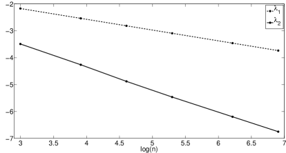
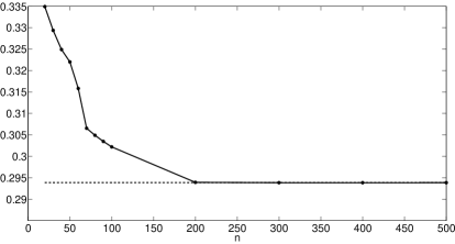
(a)	(b)

Figure 1: (a) The (fitted) plots of $e_{n}(h_{\lambda_{1}})$ (dashed-line) and $e_{n}(h_{\lambda_{2}})$ (solid line) versus $n$ in a log-log scale. (b) The convergence of $n^{0.8}e_{n}(h_{\lambda_{2}})$ (solid line) to the asymptotic constant (dashed line).

These plots correspond to the following asymptotic behavior of the approximation errors:

$$\begin{array}[]{rcl}e_{n}(h_{\lambda_{1}})&\sim&C_{1}\,n^{-0.4},\quad C_{1}\simeq 0.377,\\ e_{n}(h_{\lambda_{2}})&\sim&C_{2}\,n^{-0.8},\quad C_{2}\simeq 0.295\mbox{ as }n\to\infty.\end{array}$$

For example, the minimal number of observations needed to obtain the accuracy $0.01$ is approximately $8727$ for the equidistant sampling density $h_{\lambda_{1}}$, whereas it needs only $69$ knots when $h_{\lambda_{2}}$ is used, i.e., Theorem 1 is applicable. Figure 1(b) demonstrates the convergence of the scaled approximation error $n^{0.8}e_{n}(h_{\lambda_{2}})$ to the asymptotic constant obtained in Theorem 1.

Example 5 Let $Y(t),\,t\in[0,1]$, be a zero mean stationary Gaussian process with the covariance function $r(s,t)=\exp\{-(s-t)^{2}\}.$ We consider a distorted version of the process,

$$X(t):=t^{0.9}Y(t),\,t\in[0,1].$$

Then $X\in{\cal C}^{0,0.9}([0,1],1)\cap{\cal C}^{m}((0,1],c_{m}(\cdot))$ for any $m\geq 0$, where $c_{m}(t)=||X^{(m+1)}(t)||^{2},$ $t\in(0,1]$. The process $Y$ has infinitely many q.m. derivatives, hence the approximation rate of Hermite spline approximation is limited by the order of spline only. However, the linear methods applied to $X$ would suffer a substantial loss of efficiency. Consider now an approximation of $X$ by the composite Hermite spline $H_{1,3}$, i.e., a linear function on the interval adjacent to singularity, and the cubic Hermite spline otherwise. We investigate the mean integrated ($p=2$) approximation error $e_{n}(h_{\lambda})=e_{n}(h_{\lambda},X,H_{1,3},2)$. For the corresponding local stationarity function, we have

$$c_{3}(t)\sim Ct^{-6.2}\mbox{ as }t\to 0,$$

where $C\simeq 0.0432$. For the power density $h_{\lambda}$ and $X$, the conditions of Theorem 2 are satisfied if $\lambda>20/7$. We choose $\lambda_{2}=3$, $\lambda_{3}=4$, and $\lambda_{4}=5$ satisfying this condition, together with $\lambda_{1}=1$, the equidistant sampling density. Figure 2(a) shows the (fitted) plots and evaluated values of mean integrated errors $e_{n}(h_{\lambda_{i}})$, $i=1,2,3,4$, versus $n$ (in a log-log scale).

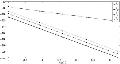
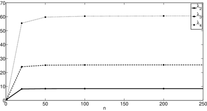
(a)	(b)

Figure 2: (a) The (fitted) plots of $e_{n}(h_{\lambda_{i}}),\,i=1,2,3,4$ versus $n$ in a log-log scale. (b) The (fitted) plots of ratios $e_{n}(h_{\lambda_{i}})/e_{n}(h^{*}),\,i=2,3,4$, for the asymptotically optimal density $h^{*}$.

Note that the estimated approximation rate for the uniform knot distribution is $n^{-1.4}$, whereas the power densities with parameters $\lambda_{2},\lambda_{3}$, and $\lambda_{4}$ result in the regular (nonsingular) case rate, namely, $n^{-4}$. By Remark 2, the asymptotically optimal density

$$h^{*}(t)=c_{3}(t)^{\frac{1}{9}}\Big{/}\int_{0}^{1}c_{3}(s)^{\frac{1}{9}}ds,\quad t\in(0,1].$$

Moreover, $h^{*}(t)\sim h_{\lambda}(t)$ with $\lambda=45/14\simeq 3.21$ as $t\to 0$. Figure 2(b) demonstrates the ratios $e_{n}(h_{\lambda_{i}})/e_{n}(h^{*}),\,i=2,3,4$ and an essential benefit in the asymptotic constant for the optimal density $h^{*}$.

4 Proofs

Proof of Theorem 1. We investigate the asymptotic behavior of the q.m. error $e_{n}(t):=||\,X(t)-H_{q,k}(X,T_{n})(t)\,||$ for any $t\in[t_{j-1},t_{j}]$, $i=1,\ldots,n$, when the number of knots $n$ tends to infinity. An explicit formula when $l=0$ or $m=0$ is used, and the q.m.  Peano kernel representation is applied otherwise. We show that the densities satisfying the conditions of the theorem lead asymptotically to eliminating the effect of the singularity point. Further, we find the asymptotic form of $||\,X-H_{q,k}(X,T_{n})\,||_{p}$ for any density $h(\cdot)$ satisfying the conditions.

Throughout the proof we utilize the next property of the Peano kernel (see, e.g., Seleznjev 2000):
Let $K_{m-1,k}(t,s),t,s\in[0,1]$, be a Peano kernel for the two-point Hermite interpolation, $m\geq 1$. If $m\leq k\leq 2m+1$, then

$$\int_{0}^{1}K^{*}_{m-1,k}(t,s)ds=0.$$ (16)

Additionally, the following (shifting) property of a regular varying function $r$ is used:
there exist positive $C,\beta$ such that

$$r(s)\leq Cr(v)\mbox{ for all }\frac{1}{2}\leq\frac{s}{v}\leq{2},\qquad v\neq 0,\,\,\max(s,v)<\beta,$$ (17)

which follows directly from the regular variation property (R1).

Note that (8) and the regular variation property (R2) imply

$$G(s)=o\left(s^{(m+\beta)/(l+\alpha+1/p)}\right)\;\mbox{ as }s\to 0.$$ (18)

Now we come to the detailed presentation of the proof. We investigate the asymptotic behaviour of the q.m.  error $e_{n}(t):=||\,X(t)-H_{q,k}(X,T_{n})(t)\,||$ for any $t\in[t_{j-1},t_{j}]$, $i=1,\ldots,n$, when the number of knots $n$ tends to infinity. Consider first the case $p=\infty$, the mean maximal norm. Let for a fixed $\delta>0$, ${J_{\delta}}$ denote the largest integer such that $t_{J_{\delta}}<\delta$. Then the error can be decomposed as follows,

$$||X-H_{q,k}(X,T_{n})||_{\infty}=\max_{[0,1]}e_{n}(t)=\max(e_{n,j},j=1,\ldots,n)=\max(S_{1},S_{2},S_{3}),$$

where $e_{n,j}:=\max_{[t_{j-1},t_{j}]}e_{n}(t)$,

$$S_{1} :=S_{1}(n)=e_{n,1},$$

$$S_{2} :=S_{2}(n)=\max(e_{n,j},j=2,\ldots,J_{\delta}),$$

$$S_{3} :=S_{3}(n)=\max(e_{n,j},j=J_{\delta}+1,\ldots,n).$$

For the first interval and $S_{1}$, if $l=0$, then a piecewise linear interpolator $H_{1}(X,T_{n})$ is applied. Hence, by the definition, (R2), (C), and (18), we obtain that

$$n^{m+\beta}e_{n,1} \leq M2^{-\alpha}n^{m+\beta}2h_{1}^{\alpha}\leq M2^{-\alpha}n^{m+\beta}G(1/n)^{\alpha}$$ (19)

$$=n^{m+\beta}\mbox{o}(n^{-(m+\beta)})=\mbox{o}(1)\mbox{ as }n\to\infty.$$

If $l>0$, Proposition 1 and (16) imply, that for $t\in[0,t_{1}]$,

$$X(t)-H_{q}(X,T_{n})(t)=h_{1}^{l}\int_{0}^{1}(Z(\bar{s})-Z(0)){K}^{*}_{l-1,q}(\bar{t},\bar{s})\;d\bar{s},$$

where $Z(\bar{s})=X^{(l)}(t_{j-1}+h_{j}\bar{s})$, and ${K}^{*}_{l-1,q}(\bar{t},\bar{s})$ denotes the corresponding Peano kernel for the two-point Hermite interpolation at $[0,1]$. Now the Hölder property and (18) give

$$n^{m+\beta}e_{1,n}\leq Cn^{m+\beta}h_{1}^{l+\alpha}=Cn^{m+\beta}G(1/n)^{l+\alpha}=\mbox{ o }(1)\mbox{ as }n\to\infty.$$ (20)

For $S_{2}$, let first $m\geq 1$. Then Proposition 1 implies

$$X(t)-H_{q,k}(X,T_{n})(t) =X(t)-H_{k}(X,T_{n})(t)=\int_{t_{j-1}}^{t_{j}}X^{(m)}(\bar{s}){K}_{m-1,k}(t,s)\;ds$$ (21)

$$=h_{j}^{m}\int_{0}^{1}Y(\bar{s}){K}^{*}_{m-1,k}(\bar{t},\bar{s})\;d\bar{s}$$

where $Y(\bar{s})=X^{(m)}(t_{j-1}+h_{j}\bar{s})$, and ${K}^{*}_{m-1,k}(\bar{t},\bar{s})$ denotes the corresponding Peano kernel for the two-point Hermite interpolation at $[0,1]$. Using (16), we get

$$X(t)-H_{q,k}(X,T_{n})(t)=h_{j}^{m}\int_{0}^{1}\left(Y(\bar{s})-Y(0)\right){K}^{*}_{m-1,k}(\bar{t},\bar{s})\;d\bar{s}.$$ (22)

Now the Cauchy-Schwartz inequality together with (2) give

$$e_{n,j}\leq Ch_{j}^{m+\beta}V(w_{j})^{1/2},$$ (23)

where $V(w_{j})^{1/2}=\max_{[t_{j-1},t_{j}]}V(t)^{1/2},w_{j}=G(s_{j})$, $s_{j}\in\left[{(j-1)}/{n},{j}/{n}\right]$, and

$$C=C(K_{m-1,k})=\max_{t\in[0,1]}||K_{m-1,k}(t,\cdot)||_{2}.$$

Notice that by definition and the integral mean value theorem for a positive $C_{1}$,

$$h_{j}=G\left(\frac{j}{n}\right)-G\left(\frac{j-1}{n}\right)=g(v_{j})\frac{1}{n}\leq C_{1}\frac{1}{n},j=1,\ldots,n,$$ (24)

and, therefore, from (22) we obtain, $v_{j}\in\left[{(j-1)}/{n},{j}/{n}\right]$,

$$n^{m+\beta}e_{n,j} \leq Cn^{m+\beta}V(w_{j})^{1/2}h_{j}^{m+\beta}\leq CV(w_{j})^{1/2}g(v_{j})^{m+\beta}$$

$$\leq CV(w_{j})^{1/2}r(v_{j})^{m+\beta}.$$

Now the (shifting) property (17) implies for some positive $C_{2}$,

$$n^{m+\beta}e_{n,j} \leq C\,V(G(s_{j}))^{1/2}r(v_{j})^{m+\beta}$$ (25)

$$\leq C_{2}V(G(s_{j}))^{1/2}r(s_{j})^{m+\beta},\;j=2,\ldots,J_{\delta},$$

for small enough $\delta$ by the definition, since $s_{j},v_{j}\in[(j-1)/{n},{j}/{n}]$ and

$$\frac{1}{2}\leq\frac{j-1}{j}\leq\frac{s_{j}}{v_{j}}\leq\frac{j}{j-1}\leq 2,\quad j\geq 2.$$

For $m=0$, we have $k=1$, and the explicit expression for the piecewise linear interpolator yields

$$e_{n,j}(t) =\,\,||X(t)-(1-\bar{t})X(t_{j-1})-\bar{t}X(t_{j})||\leq||X(t)-X(t_{j-1})||+\bar{t}||X(t_{j})-X(t_{j}-1)||$$

$$\leq(\bar{t}^{\beta}+\bar{t})V(w_{j})^{1/2}h_{j}^{\beta}\leq 2V(w_{j})^{1/2}h_{j}^{\beta},$$

and therefore, by (24), the Hölder condition, and the shifting property (17) we get

$$n^{\beta}e_{n,j}\leq 2g(v_{j})^{\beta}V(G(s_{j}))^{1/2}\leq Cr(s_{j})^{\beta}V(G(s_{j}))^{1/2},$$ (26)

for some positive constant $C$. Thus, by (C), (25), and (26) for any $\epsilon>0$, sufficiently small $\delta$, and $n$ large enough, we get

$$n^{m+\beta}S_{2}=\max(n^{m+\beta}e_{n,j},j=2,\ldots,J_{\delta})<\epsilon,$$ (27)

for any $m\geq 0$.

For $S_{3}$, we show first that

$$n^{m+\beta}S_{3}\to b^{m,\beta}_{k,\infty}\max_{[\delta,1]}(c(t)^{1/2}h^{-(m+\beta)}(t))\mbox{ as }n\to\infty.$$ (28)

The main steps of the proof repeat those of the corresponding result for a regular sequence of designs in Seleznjev (2000) for interpolation of a smooth random function by the Hermite spline $H_{k}(X,T_{n})$. Applying the local stationarity condition and uniform continuity of positive $c(t),h(t),t\in[\delta,1]$, we obtain

$$n^{m+\beta}S_{3}= n^{m+\beta}\max(e_{n}(t),t\in[t_{j-1},t_{j}],j=J_{\delta}+1,\ldots,n)$$ (29)

$$= b^{m,\beta}_{k,\infty}\max(c(w_{j})^{1/2}h(w_{j})^{-(m+\beta)},j=J_{\delta}+1,\ldots,n)(1+\mbox{o}(1)),$$

for some $w_{j}\in[t_{j-1},t_{j}],j=J_{\delta}+1,\ldots,n$, and consequently

$$n^{m+\beta}S_{3}= b^{m,\beta}_{k,\infty}\max(c(t)^{1/2}h(t)^{-(m+\beta)},t\in[t_{J_{\delta}},1])(1+\mbox{o}(1))\mbox{ as }n\to\infty.$$ (30)

Moreover,

$$\max(c(t)^{1/2}h (t)^{-(m+\beta)},t\in[t_{J_{\delta}},1])$$ (31)

$$=\max(c(t)^{1/2}h(t)^{-(m+\beta)},t\in[\delta,1])(1+\mbox{o}(1))\mbox{ as }n\to\infty,$$

since (24) yields $|t_{J_{\delta}}-\delta|\leq h_{J_{\delta}}\leq C/n$ for a positive constant $C$.
Let $a_{\delta}:=\max(c(t)^{1/2}h(t)^{-(m+\beta)},t\in[t_{J_{\delta}},1])$. Note that it follows from (C) that $a_{\delta}$ is bounded, and the monotone convergence gives

$$a_{\delta}\uparrow a:=b^{m,\beta}_{k,\infty}\sup(c(t)^{1/2}h(t)^{-(m+\beta)},t\in[0,1])\mbox{ as }\delta\to 0.$$ (32)

So, first, we select $\delta$ sufficiently small and apply (27), (30), and (32) for sufficiently large $n$. Then for the selected $\delta$, (19) and (20) imply the assertion. This completes the proof for $p=\infty$.

The proof for $1\leq p<\infty$ is analogous to the previous case, so we give the main steps only. Let for a fixed $\delta>0$,

$$e_{n}^{p}:=\int_{0}^{1}e_{n}(t)^{p}dt=\sum_{j=1}^{n}\int_{t_{j-1}}^{t_{j}}e_{n}(t)^{p}dt=e_{n,1}^{p}+\sum_{j=2}^{J_{\delta}}e_{n,j}^{p}+\sum_{j=J_{\delta}+1}^{n}e_{n,j}^{p}=S_{1}+S_{2}+S_{3},$$

where $S_{1}=S_{1}(n):=e_{n,1}$, the sum $S_{3}=S_{3}(n)$ includes all terms $e_{n,j}$ such that $[t_{j-1},t_{j}]\subset[\delta,1]$, say, $j\geq J_{\delta}+1$, and $S_{2}=e_{n}^{p}-S_{1}-S_{3}$.

For $S_{1}$, the first interval, if $l=0$, $H_{1}(X,T_{n})$ is applied, hence by the definition, (R2), (C), and (18), we have

$$n^{p(m+\beta)}(e_{n,1}(t))^{p}\leq n^{p(m+1)}M2^{-p\alpha}\int_{0}^{h_{1}}2h_{1}^{p\alpha}dt\leq M2^{1-p\alpha}n^{p(m+\beta)}G(1/n)^{p\alpha+1}$$ (33)

$$= n^{p(m+\beta)}\mbox{o}(n^{-p(m+\beta)})=\mbox{o}(1)\mbox{ as }n\to\infty.$$

If $l>0$, Proposition 1 and (16) imply that for $t\in[0,t_{1}]$,

$$X(t)-H_{q}(X,T_{n})(t)=h_{1}^{l}\int_{0}^{1}(Z(\bar{s})-Z(0)){K}^{*}_{l-1,q}(\bar{t},\bar{s})\;d\bar{s}$$

where $Z(\bar{s})=X^{(l)}(t_{j-1}+h_{j}\bar{s})$, and ${K}^{*}_{l-1,q}(\bar{t},\bar{s})$ denotes the corresponding Peano kernel for the two-point Hermite interpolation at $[0,1]$. Now the Hölder inequality and (18) give

$$n^{p(m+\beta)}(e_{n,1})^{p}\leq Cn^{p(m+\beta)}h_{1}^{1+pl+p\alpha}=Cn^{p(m+\beta)}G(1/n)^{1+pl+p\alpha}=\mbox{o}(1).$$ (34)

For $S_{2}$ and $m\geq 0$, i.e., $j=2,\ldots,J_{\delta}$, (22) and (24) yield that for some positive constant $C$

$$n^{(m+\beta)}e_{n,j}\leq Cn^{(m+\beta)}V(w_{j})^{1/2}h_{j}^{m+\beta+1/p}\leq CV(w_{j})^{1/2}g(v_{j})^{(m+\beta)}h_{j}^{1/p},$$

where $w_{j},v_{j}\in[{(j-1)}/{n},{j}/{n}]$. The (shifting) property (17) together with condition (C) imply that for some positive $C_{1}$,

$$n^{(m+\beta)p}e_{n,j}^{p}(t) \leq C^{p}V(w_{j})^{p/2}g(v_{j})^{(m+\beta)p}h_{j}\leq{C_{1}}R(s_{j})^{p}r(s_{j})^{(m+\beta)p}h_{j}$$ (35)

$$\leq C_{1}\int_{t_{j-1}}^{t_{j}}R(H(t))^{p}r(H(t))^{(m+\beta)p}dt,\;j=2,\ldots,J_{\delta},$$

where for $s_{j}=H(u_{j})\in\left[(j-1)/n,{j}/{n}\right]$,

$$R(s_{j})r(s_{j})^{m+\beta}=R(H(u_{j}))r(H(u_{j}))^{m+\beta}=\min_{[t_{j-1},t_{j}]}R(H(t))r(H(t))^{m+\beta}.$$

Thus, for any $\epsilon_{1}>0$, sufficiently small $\delta$, and large enough $n$, we obtain

$$n^{(m+\beta)p}S_{2}^{p}\leq C_{1}\int_{t_{1}}^{t_{J_{\delta}}}R(H(t))^{p}r(H(t))^{(m+\beta)p}dt<\epsilon_{1}$$ (36)

Analogously to the case $p=\infty$, the explicit form of piecewise linear interpolator is used to obtain (36) when $m=0$.

For $S_{3}$, we show that

$$n^{(m+\beta)p}S_{3}^{p}\to\left(b_{k,p}^{m,\beta}\right)^{p}\int_{\delta}^{1}c(t)^{p/2}h(t)^{-(m+\beta)p}dt\mbox{ as }n\to\infty.$$ (37)

Applying the local stationarity condition and uniform continuity of positive $c(t),h(t),t\in[\delta,1]$, we get

$$n^{(m+\beta)p}S_{3}^{p}=\left(b_{k,p}^{m,\beta}\right)^{p}\left(\sum_{j=J_{\delta}+1}^{n}c(w_{j})^{p/2}h(w_{j})^{{-(m+\beta)p}}h_{j}\right)\left(1+\mbox{o}(1)\right)$$

for some $w_{j}\in[t_{j-1},t_{j}],j=J_{\delta}+1,\ldots,n$, and consequently

$$n^{(m+\beta)p}S_{3}^{p} = \left(b_{k,p}^{m,\beta}\right)^{p}\left(\int_{t_{J_{\delta}}}^{1}c(t)^{p/2}h(t)^{{-(m+\beta)p}}dt\right)\left(1+\mbox{o}(1)\right)$$ (38)

$$= \left(b_{k,p}^{m,\beta}\right)^{p}\left(\int_{\delta}^{1}c(t)^{p/2}h(t)^{{-(m+\beta)p}}dt\right)(1+\mbox{o}(1))$$

$$=: a_{\delta}(1+\mbox{o}(1))\mbox{ as }n\to\infty.$$

Now it follows by (C), that $c(t)^{p/2}h(t)^{{-(m+\beta)p}}$ is integrable on $[0,1]$, hence

$$a_{\delta}\uparrow a:=\left(b_{k,p}^{m,\beta}\right)^{p}\int_{0}^{1}c(t)^{p/2}h(t)^{{-(m+\beta)p}}dt,t\in[0,1])\mbox{ as }\delta\to 0.$$ (39)

This completes the proof.

Proof of Theorem 2. The proof repeats the steps of that of Theorem 1 for the differentiable case. For the calculations of the asymptotic constants we refer to Seleznjev (2000).

Proof of Proposition 2. The arguments are similar for the first interval and the other intervals in both the mean integrated, and maximal norms. So we demonstrate the main steps for the $[t_{j-1},t_{j}],j\geq 2$, the mean maximal norm, and the differentiable case. Applying Proposition 1 and (16) to the Hermite spline approximation, we have, $t\in[t_{j-1},t_{j}],j\geq 2$,

$$X(t)-H_{k}(X)(t)=h_{j}^{m}\int_{0}^{1}\left(Y(\bar{s})-Y(0)\right){K}^{*}_{m-1,k}(\bar{t},\bar{s})\;d\bar{s},$$

where $Y(\bar{s})=X^{(m)}(t_{j-1}+h_{j}\bar{s})$, and ${K}^{*}_{m-1,k}(\bar{t},\bar{s})$ denotes the corresponding Peano kernel for the two-point Hermite interpolation at $[0,1]$. Now the Cauchy-Schwartz inequality, (2), and the monotonicity of $V$ give

$$||X(t)-H_{k}(X)(t)||_{\infty}\leq Ch_{j}^{m+\beta}V(t_{j-1})^{1/2},$$

where $C=C(K_{m-1,k})=\max_{t\in[0,1]}||K_{m-1,k}(t,\cdot)||_{2}$. Finally, applying the condition (15) implies the result.

References

• Abramowicz, K. and Seleznjev, O.  (2008). On the error of the Monte Carlo pricing method. J. Num. and Appl. Math. 96, 1-10

  Benhenni, K. and Cambanis, S. (1992). Sampling designs for estimating integrals of stochastic process. Ann. Statist. 20, 161-194.

  Berman, S.M.  (1974). Sojourns and extremes of Gaussian process. Ann. Probab. 2, 999- 1026; corrections 8, 999 (1980); 12, 281, (1984).

  Bingham, N.H., Goldie, C.M., and Teugels, J.L. (1987). Regular variation. Cambridge Univ. Press.

  de Boor, C. (1973). Good approximation by splines with variable knots, In: Meir, A.  and Sharma, A., Eds., Spline functions and approximation theory, Birkhäuser, 57-72.

  Buslaev, A.P. and Seleznjev, O. (1999). On certain extremal problems in theory of approximation of random processes. East J.  Approx. 5, 467–481.

  Cohen, A. and D’Ales, J.-P. (1997). Nonlinear approximation of random functions. SIAM J. Appl. Math. 57 , 518-540.

  Cohen, A., Daubechies, I., Guleryuz, O.G., and Orchard, M.T.  (2002). On the importance of combining wavelet-based nonlinear approximation with coding strategies. IEEE Trans. Inform. Theory 48 , 1895-1921.

  Creutzig, J. and Lifshits, M. (2006). Free-knot spline approximation of fractional Brownian motion. In: Keller, A., Heinrich, S., and Neiderriter, H., Eds., Monte Carlo and quasi Monte Carlo methods. Springer, Berlin, 195-204.

  Creutzig, J., Müller-Gronbach, T., and Ritter, K. (2007). Free-knot spline approximation of stochastic processes. J. Complexity 23, 867-889.

  Davis, P.J. (1975). Interpolation and approximation. Dover, New York.

  DeVore, R. (1998). Nonlinear approximation. Acta Numer. 7 , 51-150.

  Eplett, W.T. (1986). Approximation theory for simulation of continuous Gaussian processes. Prob. Theory Related Fields 73, 159-181.

  Hüsler, J. (1995). A note on extreme values of locally stationary Gaussian processes. J. Statist. Plann. Inference 45, 203- 213.

  Hüsler, J., Piterbarg, V., and Seleznjev, O. (2003). On convergence of the uniform norms for Gaussian processes and linear approximation problems. Ann. Appl. Probab. 13, 1615-1653.

  Kon, M. and Plaskota, L. (2005). Information-based nonlinear approximation: an average case setting. J. Complexity 21, 211-229,

  Ritter, K. (2000). Average-case analysis of numerical problems, Springer-Verlag.

  Sacks, J. and Ylvisaker, D.  (1966). Design for regression problems with correlated errors. Ann. Math. Statist. 37, 66-89.

  Seleznjev, O. (1996). Large deviations in the piecewise linear approximation of Gaussian processes with stationary increments. Adv. in Appl. Prob. 28, 481-499.

  Seleznjev, O. (2000). Spline approximation of random processes and design problems. J. Statist. Plann. Inference 84, 249-262.

  Su, Y. and Cambanis, S. (1993)  Sampling designs for estimation of a random process. Stoch. Proc. Appl. 46, 47-89.