Large $D-2$ Theory of Superconducting Fluctuations in a Magnetic Field and Its Application to Iron-Pnictides

Abstract

A Ginzburg-Landau approach to fluctuations of a layered superconductor in a magnetic field is used to show that the interlayer coupling can be incorporated within an interacting self-consistent theory of a single layer, in the limit of a large number of neighboring layers. The theory exhibits two phase transitions – a vortex liquid-to-solid transition is followed by a Bose-Einstein condensation into the Abrikosov lattice – illustrating the essential role of interlayer coupling. Using this theory, explicit expressions for magnetization, specific heat, and fluctuation conductivity are derived. We compare our results with recent experimental data on the iron-pnictide superconductors.

The discovery of high-temperature superconductivity in iron-pnictides kamihara08 ; pnictidereview has led to a renewed interest in the physics of layered compounds and the role of superconducting fluctuations. In older high-T_c superconducting cuprates, due in large part to their extreme anisotropy, the fluctuations have taken center stage, particularly in a magnetic field reviews . At present, a rather good understanding of such fluctations is available in two-dimensional (2D) and three-dimensional (3D) systems. However, the intermediate regime, where the interlayer coupling is too weak to be ignored and yet not strong enough to render the system fully 3D, remains an important challenge. Although most theoretical models of pnictides so far have focused on the 2D nature of these materials raghu08 ; kuroki08 ; cvetkovic09 ; Chubukov ; Bernevig , experimental evidence frequently suggests a pronounced quasi 3D behavior salem09 ; choi09 , especially within the so-called 122 family rotter08 . Thus, the iron-pnictides apparently belong to this in-between regime.

In this Letter, we introduce a theoretical approach that allows for an explicit approximate solution to the problem of superconducting fluctuations in this challenging intermediate situation. First, we show that the Josephson coupling between superconducting layers in a magnetic field can be recast as a contribution to the effective “on-site” Ginzburg-Landau (GL) free energy of a single layer, in the limit of a large number of neighboring layers. The system is thus described by an effective 2D GL theory, which – for practical purposes – can be treated exactly, by solving a set of non-linear, self-consistent equations, in combination with a solution for the purely 2D case tesanovic92 ; tesanovic94 ; ullah91 ; ikeda . Second, we show that this theory – unlike the 2D one – possesses two phase transitions, reflecting the crucial role of Josephson coupling. Finally, we apply our theory to study fluctuation effects around the upper critical field $H_{c2}(T)$ and compare the results to recent experimental data on the iron-pnictide superconductors.

We consider a general Josephson-coupled layered system, with an individual layer described by the GL model. The partition function is

$$Z=\prod_{i}\int D(\bar{\psi}_{i},\psi_{i})e^{-S_{0}(i)-\sum_{j(i)}S_{\mathrm{int}}(i,j)},$$ (1)

where $\psi_{i}\in{\rm LLL}$ is the fluctuating GL order parameter in the $i$th layer; LLL denotes the lowest Landau level for charge $2e$; and $j$ is summed over nearest neighbors of layer $i$. The corresponding action is

$$S_{0}(i)=\frac{s}{T}\int d^{2}r\left(\alpha|\psi_{i}({\bf r})|^{2}+\frac{\beta}{2}|\psi_{i}({\bf r})|^{4}\right)~{},$$ (2)

where $s$ is the distance between layers, and $\alpha=\alpha_{0}(t-t_{c2}(h))$, where $t=T/T_{c}(0)$ and $h=H/H_{c2}(0)$ are the dimensionless temperature and magnetic field, respectively. The interlayer portion of the GL-LLL action (1) is footnoteLD

$$S_{\mathrm{int}}(i,j)=-\frac{s}{T}\sum_{j=1}^{d}\int d^{2}r\frac{\eta}{2}\left[\bar{\psi}_{i}({\bf r})\psi_{j}({\bf r})+\bar{\psi}_{j}({\bf r})\psi_{i}({\bf r})\right].$$ (3)

The goal now is to integrate out the Josephson-coupled portion and obtain a partition function for the 0th layer that is entirely “local,” i.e. defined on a single layer. As a first step, we assume that this can be done for the layers (denoted by $j$) that are adjacent to the 0th layer, i.e. that all couplings $S_{int}(j,j+\sigma)$, where $\sigma$ denotes all layers neighboring layer $j$ except for the 0th layer, can be integrated over, giving a correction to the “on-site” action, so that $S_{0}(j)\rightarrow S_{0}^{\prime}(j)$. (When the number of layers $j$ is very large they decouple from each other, and we are left with a Bethe lattice, where each lattice “site” is actually a 2D superconducting layer and the coordination number of the lattice is $d$. This is different from Ref. kollar05 , where each site is a 0D quantum cluster.) We obtain

$$\begin{split}Z(0)=&\int D(\bar{\psi}_{0},\psi_{0})e^{-S_{0}(0)}\\ &\times\prod_{j=1}^{d}\frac{1}{Z_{0}(j)}\int D(\bar{\psi}_{j},\psi_{j})e^{-S^{\prime}_{0}(j)-S_{\mathrm{int}}(0,j)},\end{split}$$ (4)

where $Z_{0}(j)=Z(j)|_{S_{int}=0}$. Expanding the interlayer term in (4), and noting that only even terms in the expansion will survive the functional integration, yields

$$\begin{split}\sum_{n}\frac{1}{(2n)!}\left(\frac{\eta s}{T}\sum^{d}_{j=1}\int d^{2}r\left[\bar{\psi}_{0}({\bf r})\psi_{j}({\bf r})+\bar{\psi}_{j}({\bf r})\psi_{0}({\bf r})\right]\right)^{2n}.\end{split}$$ (5)

The terms that survive the functional integral are of the form $(\bar{\psi}_{0}\psi_{0})^{n}\bar{\psi}_{j_{1}}\psi_{j_{1}}\dots\bar{\psi}_{j_{n}}\psi_{j_{n}}$. In the $d\to\infty$ limit, the large majority of these terms has $j_{1}\neq j_{2}\neq\dots\neq j_{n}$. There are $(2n)!$ of each terms of this type. Since each involves $n$ pairs, and since there are $d$ possible pairs to choose from, the total number of all such terms (note that $j$’s are indistinguishable) is $(2n)!\binom{d}{n}\xrightarrow{d\rightarrow\infty}(2n)!d^{n}/n!$.

Thus, in the large-$d$ limit (5) turns into

$$\begin{split}&\sum_{n}\frac{1}{(2n)!}\left(\frac{\eta s}{T}\right)^{2n}\frac{d^{n}(2n)!}{n!}\left(\int D(\bar{\psi}_{j},\psi_{j})e^{-S^{\prime}_{0}(j)}\right)^{d-n}\\ &\times\left(\int D(\bar{\psi}_{j},\psi_{j})e^{-S^{\prime}_{0}(j)}\int d^{2}r\int d^{2}r^{\prime}\bar{\psi}_{0}\psi_{0}^{\prime}\bar{\psi}_{j}\psi_{j}^{\prime}\right)^{n},\end{split}$$ (6)

where we have adopted the shorthand $\psi\equiv\psi({\bf r})$ and $\psi^{\prime}\equiv\psi({\bf r}^{\prime})$. This expression can now be inserted into Eq. (4), where the sum over $n$ can be re-exponentiated, giving

$$\begin{split}Z^{(1)}(0)=&\int D(\bar{\psi},\psi)e^{-S_{0}}\\ &\times\exp{\left[\left(\frac{\tilde{\eta}s}{T}\right)^{2}\int d^{2}r\int d^{2}r^{\prime}\bar{\psi}\psi^{\prime}\left<\bar{\psi}\psi^{\prime}\right>\right]}.\end{split}$$ (7)

The superscript in $Z^{(1)}(0)$ signifies that this is the leading term in a large-$d$ expansion. Here we have defined $\tilde{\eta}\equiv\eta\sqrt{d}$ as the new interlayer coupling, which remains finite as $\eta\rightarrow 0$ and $d\rightarrow\infty$. The $j$ index has been dropped, since all layers are equivalent and are no longer coupled. The general correlation function is defined as

$$\left<\dots\right>\equiv\frac{\int D(\bar{\psi},\psi)(\dots)e^{-S^{\prime}_{0}}}{\int D(\bar{\psi},\psi)e^{-S^{\prime}_{0}}}.$$ (8)

In the symmetric gauge, the correlation function in (7) is

$$\left<\bar{\psi}({\bf r})\psi({\bf r}^{\prime})\right>=\frac{T}{2\pi l^{2}s\tilde{\alpha}}e^{-(|z|^{2}+|z^{\prime}|^{2})/4+\bar{z}z^{\prime}/2}.$$ (9)

where $z=(x+iy)/l$ is the complex coordinate within a single layer, $l=\sqrt{\phi_{0}/2\pi H}$ is the magnetic length, and $\tilde{\alpha}$ is defined later. The integral in Eq. (7) is thus

$$\begin{split}&\frac{1}{\tilde{\alpha}}\int d^{2}r\int d^{2}r^{\prime}\bar{\psi}({\bf r})\psi({\bf r}^{\prime})e^{-(|z|^{2}+|z^{\prime}|^{2})/4+\bar{z}z^{\prime}/2}\\ &=\frac{2\pi l^{2}}{\tilde{\alpha}}\int d^{2}r|\psi({\bf r})|^{2}.\end{split}$$ (10)

The last equality follows from $\psi\in{\rm LLL}$.

Following Ref. tesanovic94 , we make change of variables ${\psi({\bf r})=\Phi\prod_{i}(z-z_{i})e^{-|z|^{2}/4}}$, where $\{z_{i}\}$ are the positions of vortices. The interaction of $\{z_{i}\}$ is set by $U^{-1}\equiv\sqrt{\left<\beta_{A}\right>}$, where $\beta_{A}(\{z_{i}\})\equiv\overline{|\psi|^{4}}/\overline{|\psi|^{2}}^{2}$ is the Abrikosov ratio for arbitrary $\{z_{i}\}$ ($\overline{\cdots}$ denotes a spatial average). The partition function for the zeroth layer becomes

$$\begin{split}&Z^{(1)}(0)=\int d\Phi^{*}d\Phi\int dUe^{Ns(U)}e^{-S_{\mathrm{eff}}}\\ &S_{\mathrm{eff}}=\frac{2\pi l^{2}sN}{T}\left(\alpha^{\prime}|\Phi|^{2}+\frac{\beta}{2U^{2}}|\Phi|^{4}\right)-N\mathrm{ln}(2\pi l^{2}s|\Phi|^{2})\end{split}$$ (11)

Here $N$ is the number of vortices $\{z_{i}\}$ and $\alpha^{\prime}\equiv\alpha-\tilde{\eta}^{2}/\tilde{\alpha}$. The entropy function $s(U)$ contains all the effects of lateral correlations among vortices $\{z_{i}\}$, and knowledge of its exact form is equivalent to the exact solution for the thermodynamics of a single layer tesanovic94 .

In the thermodynamic limit $N\to\infty$, the saddle point method can be applied to integrals over $\Phi$ and $U$ in Eq. (LABEL:z_phi). Minimizing with respect to $|\Phi|^{2}$ gives

$$|\Phi_{0}|^{2}=\frac{1}{2}\left[-\frac{\alpha^{\prime}U^{2}}{\beta}+\sqrt{\left(\frac{\alpha^{\prime}U^{2}}{\beta}\right)^{2}+\frac{4TU^{2}}{2\pi l^{2}s\beta}}\right].$$ (12)

In order for this expression to be useful, we must determine the form of $\tilde{\alpha}$, as well as $U$.

From Eq. (9), we have $\tilde{\alpha}^{-1}=(2\pi l^{2}s/T)\left<\bar{\psi}(0)\psi(0)\right>$. Using this along with Eqs. (8) and (12), we obtain the following self-consistent expression for $\tilde{\alpha}$:

$$\tilde{\alpha}=\alpha-\frac{\tilde{\eta}^{2}}{\tilde{\alpha}}+\frac{\beta T}{2\pi l^{2}s\tilde{\alpha}U^{2}}.$$ (13)

Solving this for $\tilde{\alpha}$, and substituting the result into our expression for $\alpha^{\prime}$, we get

$$\alpha^{\prime}=\alpha\left[1-\frac{2\left(\frac{\tilde{\eta}}{\alpha}\right)^{2}}{1+\mathrm{sgn}(\alpha)\sqrt{1+\frac{2}{\alpha^{2}}\left(\frac{\beta T}{\pi l^{2}sU^{2}}-2\tilde{\eta}^{2}\right)}}\right].$$ (14)

In solving for this expression, we must assume $\beta^{\prime}\equiv\beta-2\tilde{\eta}^{2}(\pi l^{2}sU^{2}/T)>0$. $\beta^{\prime}<0$ leads to $\tilde{\alpha}<0$, which is clearly unphysical. The implications of $\beta^{\prime}\to 0^{+}$ at finite $T$ are important and are discussed shortly. Eq. (14) constitutes our main theoretical result, allowing us to describe the system of coupled layers with a 2D GL-LLL action, albeit with $\alpha\rightarrow\alpha^{\prime}$. Its innocent appearance notwithstanding, the change $\alpha\rightarrow\alpha^{\prime}$ actually entails an elaborate self-consistent calculation to determine the ultimate dependence on $T$ and $H$. Note that the next term in the large-$d$ expansion – arising from terms in (5) with one index repeated four times – modifies the quartic term $\beta$ in the 2D GL action. It is important to systematically incorporate such finite-$d$ corrections when addressing the details of interlayer correlations in real materials.

Evaluating Eq. (LABEL:z_phi) at its saddle point and using Eq. (12), we obtain for the free energy density

$$\begin{split}\frac{F}{V}=&\frac{HT}{\phi_{0}s}\Bigg{[}\frac{1}{2}-\frac{1}{2}g^{2}U^{2}+\frac{1}{2}gU\sqrt{2+g^{2}U^{2}}\\ &-\mathrm{ln}\left(-gU^{2}+U\sqrt{2+g^{2}U^{2}}\right)-\frac{1}{2}\mathrm{ln}\frac{\pi l^{2}sT}{\beta}\Bigg{]},\end{split}$$ (15)

where $g\equiv\alpha^{\prime}\sqrt{2\pi l^{2}s/(2\beta T)}$ can be expressed using Eq. (14) as

$$g=g_{0}\frac{t-t_{c2}(h)}{\sqrt{ht}}\left[1-\frac{\frac{2}{(t-t_{c2}(h))^{2}}\left(\frac{\tilde{\eta}}{\alpha_{0}}\right)^{2}}{\mathrm{sgn}(\alpha)\Xi(h,t)+1}\right].$$ (16)

In the above equation $g_{0}\equiv\sqrt{s\phi_{0}H_{c2}(0)/16\pi\kappa^{2}T_{c}(0)}$,

$$\Xi(h,t)\equiv\left[1+\frac{4}{(t-t_{c2}(h))^{2}}\left(\frac{ht}{2g_{0}^{2}U^{2}(g)}-\left(\frac{\tilde{\eta}}{\alpha_{0}}\right)^{2}\right)\right]^{1/2},$$ (17)

and we used the GL result $\alpha_{0}^{2}/\beta=H_{c2}^{2}(0)/8\pi\kappa^{2}$ tinkham96 .

$g(t,h)$ (16) is the scaling variable of our theory. Since $\Xi(h,t)$ depends on $U(g)$, Eq. (16) has the form $g=g(U(g))$. $U(g)$ is the same as in a purely 2D problem, but there $g(t,h)=g_{0}(t-t_{c2}(h))/\sqrt{ht}$, so the $t$ and $h$ dependencies in our case are very different. $U(g)$ follows from minimization of (LABEL:z_phi) and relies on knowledge of $s(U)$. Here we can turn the problem around and exploit the fact that $\beta_{A}(g)$ interpolates between its high- and low-$T$ limits of 2 and $\beta_{\Delta}\equiv 1.159$, respectively. In particular,

$$U(g)=0.818-0.110\ \mathrm{tanh}\left(\frac{g+c_{1}}{c_{2}}\right),$$ (18)

suggested in Ref. tesanovic94 , where $c_{1}=1.60$ and $c_{2}=2.66$ from the fit to the Monte Carlo results of Ref. kato93 , yields a virtually exact solution for fluctuation thermodynamics footnote . This expression for $U(g)$ can then be used to solve self-consistently for $g$ in Eq. (16).

It is now clear that the divergence in Eq. (14), associated with $\beta^{\prime}\to 0^{+}$ and $T\to T_{\Delta}=2\pi l^{2}\tilde{\eta}^{2}s/(\beta\beta_{\Delta})$, is endowed with special significance. As $T$ is lowered toward $T_{\Delta}$, $g\rightarrow-\infty$ (since $g\propto\alpha^{\prime}$), and thus $U(g)\rightarrow 1/\sqrt{\beta_{\Delta}}$. Therefore, at finite temperature $T_{\Delta}$ the system undergoes a Bose-Einstein condensation transition into the Abrikosov lattice state. In a purely 2D ($\tilde{\eta}=0$) theory, such a transition could occur only at $T=0$. Once $\tilde{\eta}\not=0$, this transition moves to finite $T_{\Delta}$, which, over a large portion of an $H-T$ phase diagram, is far below the vortex liquid-solid transition taking place at $T_{M}$, defined by $g=g_{M}\sim-7$ footnote . As $H\to 0$, both $T_{\Delta}$ and $T_{M}$ tend into $T_{c2}(H)$. This echoes the phase diagram of layered superconductors proposed in Ref. tesanovic94a .

We now turn our attention to fluctuation thermodynamics tesanovic94 ; kogan ; koshelev . The magnetization follows from $4\pi M=-(1/V)\partial F/\partial H$, with $|\Phi_{0}|^{2}$ given in (12):

$$\frac{4\pi\phi_{0}sM}{T_{c}(0)}=g_{0}\sqrt{ht}\left(gU^{2}-U\sqrt{2+g^{2}U^{2}}\right).$$ (19)

Fig. 1 shows fluctuation magnetization data choi09 for $\mathrm{BaFe_{1.8}Co_{0.2}As_{2}}$, and a fit of Eq. (19) to the data. For this sample $T_{c}(0)=23.6\ \mathrm{K}$; and we obtain $g_{0}=5.8$ using the values $H_{c2}(0)=72\ \mathrm{T}$ for the upper critical field, $\kappa=44$ for the GL parameter williams09 , and $s=6.65\ \mathrm{\AA}$ for the interlayer spacing rotter08 . The demagnetization factor $D_{M}$, which reduces the overall magnetization by a factor of $1-D_{M}$, is not known exactly for this sample, but can be estimated as $D_{M}\approx 1-\pi d/(2R)$, which is valid for a flat disk of radius $R$ and thickness $d\ll R$ in a perpendicular magnetic field fetter67 . The sample used in Ref. choi09 is rectangular in shape with length and width $L\approx 10d$, so we expect $D_{M}\approx 1-\pi/10$.

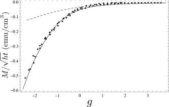
Figure 1: Scaled magnetization data from Ref. choi09 , at fields 3, 5, and 7 T, along with a theoretical fit from Eq. (19). The theoretical scaling function (19) uses fitting parameters $D_{M}=0.70$ and $\tilde{\eta}/\alpha_{0}=0.034$ (solid line), with other parameters given in the text. The dashed line is the 2D case ($\tilde{\eta}=0$).

Fitting the data with respect to $D_{M}$ and $\tilde{\eta}/\alpha_{0}$, with other parameters fixed, yields the curve in Fig. 1 and $D_{M}=0.70$, $\tilde{\eta}/\alpha_{0}=0.034$.

We now calculate the heat capacity $C=-T\partial^{2}F/\partial T^{2}$. From Eq. (15) we obtain

$$\begin{split}\frac{2g_{0}^{2}}{h\beta_{\Delta}}c=&\left(2\frac{\partial g}{\partial t}+t\frac{\partial^{2}g}{\partial t^{2}}\right)\left(2gU^{2}-2U\sqrt{2+g^{2}U^{2}}\right)\\ &+\frac{1}{2t}+2t\left(\frac{\partial g}{\partial t}\right)^{2}\left(U^{2}-\frac{gU^{3}}{\sqrt{2+g^{2}U^{2}}}\right)\\ &+4t\left(\frac{\partial g}{\partial t}\right)^{2}\frac{dU}{dg}\left(gU-\frac{1+g^{2}U^{2}}{\sqrt{2+g^{2}U^{2}}}\right).\end{split}$$ (20)

Here the heat capacity $c\equiv C/\Delta C_{2d}$ has been normalized to its 2D mean-field value, $\Delta C_{2d}=V\alpha_{0}^{2}t/(s\beta\beta_{\Delta})=2VH_{c2}(0)g_{0}^{2}t/(\phi_{0}s\beta_{\Delta})$, and $g$ is given by (16). Fig. 2 shows $c$ for three different values of $\tilde{\eta}$. As $T\to 0$, there is a divergence in the specific heat, stemming from the fact that, for $\tilde{\eta}\not=0$, $g\rightarrow-\infty$ at finite $T\to T_{\Delta}$, as discussed before. This is suggestive of a first-order Abrikosov transition at $T_{\Delta}$; to describe its details our approach needs to be augmented either by the sixth order GL term (since $\beta^{\prime}\to 0^{+}$ at $T_{\Delta}$) or finite $d$ corrections, something left for future study. The specific heat, being a second derivative, is rather sensitive to this divergence at low $T$, even for small $\tilde{\eta}$, as we illustrate in the figure.

Recent experiments on $\mathrm{SmFeAsO_{1-x}F_{x}}$ pallecchi09 suggest that the fluctuation conductivity follows an approximate 2D scaling behavior of the form predicted by Ref. ullah91 (see also Ref. ikeda ), where transport coefficients are derived from the time-dependent GL-LLL theory, within the Hartree-Fock approximation ($\beta_{A}=2$). We follow Ref. ullah91 to obtain the fluctuation conductivity as

$$\sqrt{\frac{H}{T}}\Delta\sigma_{yy}=\frac{\hbar}{64\lambda_{ab}(0)\xi_{ab}(0)T_{c}(0)}\sqrt{\frac{\pi}{s\phi_{0}}}{\cal K}(g),$$ (21)

where, in their case, the scaling variable $g$ has its 2D form, i.e. $\tilde{\eta}=0$ in Eq. (16).

Figure 2: Specific heat from Eq. (20), with $g_{0}=3$, $h=0.3$, and $t_{c2}(h)=1-h$. The three curves have interlayer coupling values of $\tilde{\eta}/\alpha_{0}=0$ (solid), 0.002 (dashed), and 0.004 (dotted).

In obtaining Eq. (21), we used the relations from the GL theory $\alpha_{0}=e^{2}H_{c2}^{2}(0)\lambda_{ab}^{2}(0)/m_{ab}c^{2}\kappa^{2}$ and $H_{c2}(0)=\phi_{0}/2\pi\xi_{ab}^{2}(0)$, as well as the expression for the coefficient in the time-dependent GL equation $\Gamma_{0}^{-1}\approx\pi\hbar\alpha_{0}/8T_{c}(0)$ tinkham96 ; larkin05 . The scaling function in (21) has the form ${\cal K}(g)={\cal K}_{2D}(g)\equiv-g/2+\sqrt{1+g^{2}/4}$, where now, of course, the scaling variable $g$ must be changed to our Eq. (16), with $\tilde{\eta}\not=0$.

Comparison of the scaling function ${\cal K}(g)$ to the experimental data in pallecchi09 is not straightforward since their sample is a polycrystal. To compensate for this, we replace $\xi_{ab}(0)\to(\xi_{ab}(0)^{2}\xi_{c}(0))^{1/3}$, $\lambda_{ab}(0)\to(\lambda_{ab}(0)^{2}\lambda_{c}(0))^{1/3}$ in the prefactor in (21). Fig. 3 shows ${\cal K}(g)$ and the data for the optimally doped ($x=0.15$, $T_{c}(0)=51.5\ \mathrm{K}$) sample at $H=28\ \mathrm{T}$. The coherence length is $\xi_{ab(c)}(0)=24\ (3)\ \mathrm{\AA}$ pallecchi09 ; the penetration depth $\lambda_{ab(c)}(0)=2000\ (16000)\ \mathrm{\AA}$ prozorov09 ; the upper critical field $H_{c2}(0)/T_{c}(0)=7.8\ \mathrm{T/K}$ footnotehighslope fits snugly between $|dH^{10\%}_{c2}/dT|$ and $|dH^{90\%}_{c2}/dT|$ reported in Ref. pallecchi09 ; and the interlayer separation $s=8.45\mathrm{\AA}$ margadonna09 .

Figure 3: Fluctuation conductivity data from Ref. pallecchi09 , along with a theoretical fit, with scaling variable $g$ from (16), $g_{0}=6.37$, and $\tilde{\eta}/\alpha_{0}=0.022$ (solid line). The purely 2D curve ($\tilde{\eta}=0$) is shown for comparison (dashed line). Other parameters are given in the text.

One can see that the interlayer coupling leads to a strong enhancement of conductivity over its 2D form, even for modest values of $\tilde{\eta}/\alpha_{0}$.

In summary, we showed that a GL theory of coupled fluctuating superconducting layers in a magnetic field can be expressed as an effective, self-consistent single layer problem, in the limit of a large number of neighboring layers. Our approach can be generalized to other 2D, 1+1D or 2+1D problems. Comparison of the theory with experimental results in the iron-pnictides is rather favorable, and provides a means of making the quasi 3D nature of these materials more theoretically tractable.

References

(1) Y. Kamihara et al., J. Am. Chem. Soc. 130, 3296 (2008).
(2) P. C. W. Chu et al. (eds.), Superconductivity in iron-pnictides. Physica C 469 (special issue), 313-674 (2009).
(3) G. Blatter et al., Rev. Mod. Phys 66, 1125 (1994);
B. Rosenstein and D. Li, Rev. Mod. Phys. 82 109 (2010).
(4) S. Raghu et al., Phys. Rev. B 77, 220503 (2008).
(5) K. Kuroki et al., Phys. Rev. Lett. 101, 087004 (2008).
(6) V. Cvetković and Z. Tešanović, Europhys. Lett. 85, 37002 (2009).
(7) A.V. Chubukov et al., Phys. Rev. B, 78,134512 (2008).
(8) M. M. Parish et al., Phys. Rev. B 78, 144514 (2008).
(9) C. Choi et al., Supercond. Sci. Technol. 22, 105016 (2009).
(10) S. Salem-Sugui, Jr. et al., Phys. Rev. B 80, 014518 (2009).
(11) M. Rotter et al., Phys. Rev. Lett. 101, 107006 (2008).
(12) Z. Tešanović and A. Andreev, Phys. Rev. B 49, 4064 (1994).
(13) Z. Tešanović et al.,
Phys. Rev. Lett. 69, 3563 (1992).
(14) S. Ullah and A. Dorsey, Phys. Rev. B 44, 262 (1991).
(15) R. Ikeda et al., J. Phys. Soc. Jpn. 60, 1051 (1991).
(16) The renormalization of from the familiar Lawrence-Doniach term (W. E. Lawrence and S. Doniach, in Proc. 12th Int. Conf. Low Temp. Phys., (Kyoto, 1970)) is absorbed into the definition of .
(17) M. Kollar et al., Ann. Phys. (Leipzig) 14, 642 (2005).
(18) M. Tinkham, Introduction to Superconductivity (Dover, 1996).
(19) Y. Kato and N. Nagaosa, Phys. Rev. B 48, 7383 (1993).
(20) The thermodynamics thus obtained is within 1-2% of
numerical simulations.
If even better accuracy is needed, a more elaborate form
of can be used, including one that allows for a 2D vortex liquid-to-solid
transition at (See
Z. Tešanović and L. Xing, Phys. Rev. Lett. 67, 2729 (1991),
J. Hu and A. H. MacDonald, Phys. Rev. Lett. 71, 432 (1993),
and kato93 ).
(21) Z. Tešanović, Physica C 220, 303 (1994).
(22) L. N. Bulaevskii et al.,
Phys. Rev. Lett. 68, 3773 (1992).
(23) A. E. Koshelev, Phys. Rev. B 50, 506 (1994).
(24) T. J. Williams et al., Phys. Rev. B 80, 094501 (2009).
(25) A. L. Fetter and P. C. Hohenberg, Phys Rev. 159, 330 (1967).
(26) I. Pallecchi et al., Phys. Rev. B 79, 104515 (2009).
(27) A. Larkin and A. Varlamov, Theory of Fluctuations in Superconductors (Oxford University Press, 2005).
(28) S. Weyeneth et al., J. Supercond.
Nov. Magn. 22, 325 (2009);
R. Prozorov et al., Physica C 469, 582 (2009).
(29) Note that such
a high value of simply reflects
a polycrystalline character of a sample used in Ref. pallecchi09 , with
.
(30) S. Margadonna et al., Phys. Rev. B 79, 014503 (2009).