Spatial Rock–Paper–Scissors Models with Inhomogeneous Reaction Rates

Abstract

We study several variants of the stochastic four-state rock–paper–scissors game or, equivalently, cyclic three-species predator–prey models with conserved total particle density, by means of Monte Carlo simulations on one- and two-dimensional lattices. Specifically, we investigate the influence of spatial variability of the reaction rates and site occupancy restrictions on the transient oscillations of the species densities and on spatial correlation functions in the quasi-stationary coexistence state. For small systems, we also numerically determine the dependence of typical extinction times on the number of lattice sites. In stark contrast with two-species stochastic Lotka–Volterra systems, we find that for our three-species models with cyclic competition quenched disorder in the reaction rates has very little effect on the dynamics and the long-time properties of the coexistence state. Similarly, we observe that site restriction only has a minor influence on the system’s dynamical properties. Our results therefore demonstrate that the features of the spatial rock–paper–scissors system are remarkably robust with respect to model variations, and stochastic fluctuations as well as spatial correlations play a comparatively minor role.

I Introduction

Understanding the origin of and maintaining biodiversity is of obvious paramount importance in ecology and biology May ; Maynard ; Michod ; Sole ; Neal . In this context, paradigmatic schematic models of predator–prey interaction that build on the classic Lotka–Volterra system Lotka ; Volterra have been widely studied. Specifically, systems with cyclic dominance of competing populations have been suggested to provide a mechanism to promote species diversity; there are also natural connections to evolutionary game theory MaynardSmith ; Hofbauer ; Nowak ; Szabo ; Redner ; Mobilia . A minimal yet non-trivial model for cyclic competition is the three-species cyclic predator–prey system with standard Lotka–Volterra predation interactions, essentially equivalent to the familiar rock–paper–scissors (RPS) game MaynardSmith ; Hofbauer ; Nowak ; Szabo . This RPS system has, for example, been used to model the cyclic competitions between three subspecies of certain Californian lizards Sinervo ; Zamudio , and the coevolution of three strains of E. coli bacteria in microbial experiments Kerr . Other examples include coral reef invertebrates Jackson and overgrowths by marine sessile organisms Buss ; Burrows . In this simple RPS model, one lets ‘rock’ (species $A$) smash ‘scissors’ (species $B$), ‘scissors’ cut ‘paper’ (species $C$), and ‘paper’ wrap ‘rock’. Already for a non-spatial RPS system, the presence of intrinsic stochastic fluctuations (reaction noise) makes the system eventually evolve to one of the three extinction states where only one species survives Ifti ; Reichen ; Frean ; Berr . For example, if the reaction rates in the system are not equal, one intriguingly observes the ‘weakest’ species, with the smallest predation rate, to survive, whereas the other two species always die out Berr ; Frean . When the model is extended to include spatial degrees of freedom, say by allowing particles to hop to nearest-neighbor sites on a lattice and interact upon encounter, spatial fluctuations and correlations further complicate the picture. For instance, species extinction still prevails in one-dimensional RPS models Tainaka1 ; Frache1 ; Frache2 ; Provata , but the system settles in a coexistence state when the species are efficiently mixed through particle exchange (but see also Ref. Pleimling ). In contrast, two-dimensional RPS systems are characterized by coexistence of the competing species, and the emergence of complex spatio-temporal structures such as spiral patterns Frean ; Tainaka1 ; Provata ; Tainaka2 ; Tainaka3 ; Szabo2 ; Perc ; Reichenbach1 ; Reichenbach2 ; Reichenbach3 ; Reichenbach4 ; Tsekouras ; Matti . Recently, Reichenbach et al. extensively studied the four-state RPS model without conservation law Reichenbach1 ; Reichenbach2 ; Reichenbach3 ; Reichenbach4 , and it is now well-established that cyclic reactions in conjunction with diffusive spreading generate spiral patterns (when the system is sufficiently mixed). In model variants that incorporate conservation of the total population density, on the other hand, spiral patterns do not occur Tainaka1 ; Frean ; Matti ; also, when the species mobility is drastically enhanced through fast particle exchange processes, the spiral patterns are destroyed as well, and the system eventually reaches an extinction state Reichenbach1 ; Matti .

This work is motivated by the following question: Which are the crucial model ingredients to be included in order to attain a further degree of realism? To this end, we carried out Monte Carlo simulation studies on the influence of the carrying capacity and environmental inhomogeneity on the properties of a class of spatial RPS models where the total population size is conserved (zero-sum games) Hofbauer ; Szabo ; Ifti ; Reichenbach1 ; Frean ; Tainaka1 ; Frache1 ; Frache2 ; Provata ; Tainaka2 ; Tainaka3 ; Tsekouras ; Matti ; Dobrienski . In our stochastic lattice models, the carrying capacity (i.e., the maximum population size that can be sustained by the environment) is implemented through site occupation number restrictions. Environmental variability is modeled through assigning local reaction rates that are treated as quenched random variables drawn from a uniform distribution. Our extensive numerical study shows that carrying capacity and quenched disorder have little influence on the oscillatory dynamics, spatial correlation functions, and extinction times in the RPS model system. This demonstrates a quite remarkable robustness of this class of models. From a modeling perspective, this establishes the essential equivalence of rather distinct model variants. We emphasize that this outcome is nontrivial, as is, for example, revealed by a comparison with the two-species Lotka-Volterra system Ivan ; Mark , where spatially varying reaction rates may cause more localized clusters of activity and thereby enhance the fitness of both predator and prey species Ulrich .

Naturally, lattice models should be viewed as coarse-grained representations of a metapopulation system where each lattice site or cell can be interpreted as a ‘patch’ (or ‘island’) populated by a ‘deme’ (or ‘local community’) Hubbell ; Hanski . For the sake of simplicity (i.e. to try to understand the simplest possible systems before venturing further), we here restrict our presentation to RPS model variants that obey a conservation law (even though that has no particular ecological motivation). As empty lattice sites are allowed, we shall refer to our model system as a class of four-state RPS models with conservation law (if all sites are at most occupied by a single individual, each of them can be in one of four states). While the presence or absence of the conservation of the total number of particles is crucial for the emergence of spiral waves in RPS systems Matti , this is not the case for the properties studied here. In fact, it turns out that our conclusions on the effects (or lack thereof) of limited carrying capacity and random environmental influences on the transient population oscillations, spatial correlation functions, and species extinction times are common to models both with and without conservation laws HMT .

Our paper is structured as follows: In Sec. II, we define our model, the stochastic four-state spatial rock–paper–scissors (RPS) game or cyclic three-species predator–prey system with conservation of total population density, and briefly review the results obtained from the mean-field rate equation approximation. In Sec. III, we introduce our Monte Carlo simulation algorithm and discuss the detailed model variants we have explored. We then present results for the species’ time-dependent densities, associated frequency power spectra, and spatial correlation functions to analyze the influence of quenched spatial disorder in the reaction rates and site occupation restriction on the temporal evolution and quasi-stationary states of this system, both in two dimensions and for a one-dimensional lattice. We also compare our numerical findings with the mean-field predictions, and obtain the mean extinction time (for the first species to die out) as function of system size. Finally, we provide a summary of our results and concluding remarks.

II Model and rate equations

The rock–paper–scissors (RPS) model describes the cyclic competition of three interacting species that we label $A$, $B$, and $C$. We consider the following (zero-sum Hofbauer ) predator–prey type interactions:

$$A+B \to A+A\quad{\rm with\ rate}\ k_{a}\ ,$$

$$B+C \to B+B\quad{\rm with\ rate}\ k_{b}\ ,$$ (1)

$$C+A \to C+C\quad{\rm with\ rate}\ k_{c}\ .$$

Note that these irreversible reactions strictly conserve the total number of particles. We remark that naturally other variants of the RPS dynamics could also be considered; notably the four-state May–Leonard model which does not conserve the total particle density MayLeonard has attracted considerable attention, see e.g. Refs. Hofbauer ; DurrettLevin ; Reichenbach2 . As will be demonstrated elsewhere, the conclusions presented here on the effects of carrying capacity and spatial reaction rate variability remain essentially unchanged for this system HMT . To generalize the above reaction model to a spatially extended lattice version, we allow empty sites (as a fourth possible state) and let the reactions happen only between nearest neighbors. In addition, we introduce nearest-neighbor particle hopping with rate $D$ (if at most one particle is allowed per lattice site, this process takes place only if an adjacent empty site becomes selected at each time step).

Within the mean-field approximation, wherein any correlations and spatial variations are neglected, the following set of three coupled rate equations for homogeneous population densities $a(t)$, $b(t)$, and $c(t)$, with fixed total population density $a(t)+b(t)+c(t)=\rho={\rm const}$ describes the system’s temporal evolution,

$$\partial_{t}\,a(t) = a(t)\left[k_{a}\,b(t)-k_{c}\,c(t)\right]\,,$$

$$\partial_{t}\,b(t) = b(t)\left[k_{b}\,c(t)-k_{a}\,a(t)\right]\,,$$ (2)

$$\partial_{t}\,c(t) = c(t)\left[k_{c}\,a(t)-k_{b}\,b(t)\right]\,.$$

These coupled rate equations possess a reactive fixed point, where all three species coexist, $(a^{*},b^{*},c^{*})=(k_{b},k_{c},k_{a})\rho/(k_{a}+k_{b}+k_{c})$, which is marginally stable (see also Ref. Frean ). Indeed, introducing new variables $\delta a(t)=a(t)-a^{*}$, $\delta b(t)=b(t)-b^{*},$ $\delta c(t)=c(t)-c^{*}$, and utilizing the conservation law $\delta a+\delta b+\delta c=0$, we may express the first two rate equations in terms of $\delta a$ and $\delta b$. Linearizing about the reactive fixed point then gives

$$\left(\begin{array}[]{c}\partial_{t}\,{\delta a}\\ \partial_{t}\,{\delta b}\\ \end{array}\right)=L\left(\begin{array}[]{c}\delta a\\ \delta b\\ \end{array}\right)\ ,$$ (3)

with the linear stability matrix

$$L=\frac{\rho}{k_{a}+k_{b}+k_{c}}\left(\begin{array}[]{cc}k_{b}\,k_{c}&k_{b}\,(k_{a}+k_{c})\\ -k_{c}\,(k_{a}+k_{b})&-k_{b}\,k_{c}\\ \end{array}\right)\ ,$$ (4)

with eigenvalues $\lambda=\pm i\,\rho\,\sqrt{k_{a}\,k_{b}\,k_{c}/(k_{a}+k_{b}+k_{c})}=\pm i\omega$, where $f=\omega/2\pi$ represents a characteristic oscillation frequency, e.g., for total density $\rho=1$ and $k_{a}=0.2$, $k_{b}=0.5$, $k_{c}=0.8$, $\lambda=\pm i\,2\sqrt{3}/15$, and the typical frequency is $f\approx 0.037$. We will use these mean-field values later to compare with the simulation results. In the special case of symmetric reaction rates where $k_{a}=k_{b}=k_{c}=k$, we get $\lambda=\pm i\,k/\sqrt{3}$; for example, if $\rho=1$ and $k=0.5$, then $\lambda=\pm i\,\sqrt{3}/6$ and $f\approx 0.046$. In addition, the system also has three absorbing states, with only a single species surviving ultimately: $(\rho,0,0)$, $(0,\rho,0)$, and $(0,0,\rho)$. Within the mean-field approximation, these fixed points are all linearly unstable. However, in any stochastic model realization on a finite lattice, temporal evolution would ultimately terminate in one of these absorbing states, as we shall explore for small systems below.

III Monte Carlo simulation results

III.1 Model variants and quantities of interest

We investigate stochastic RPS systems on one- and two-dimensional lattices with periodic boundary conditions. At each time step, one individual of any species is selected at random, then hops to a nearest-neighbor site, if the number of particles on the chosen target site is empty. Otherwise, one of the particles on the chosen neighboring site is selected randomly and undergoes a reaction with the center particle according to the scheme and rates specified by (1) if both particles are different. The outcome of the reaction then replaces the eliminated particle. Note that predation reactions always involve neighboring particles; on-site reactions do not occur. This has the advantage of permitting us to treat the model variants with and without site occupation number restriction within the same setup, allowing for direct comparison. A similar approach was already adopted for the two-species lattice Lotka–Volterra model, where we confirmed earlier that nearest-neighbor predation interactions and strictly on-site reactions lead (without loss of generality) to essentially identical macroscopic features Ivan ; Mark .

If the selected and focal particle are of the same species, the center particle just hops to its chosen neighboring site. For our model variants with site occupancy restriction, the hopping process only takes place if the total number of particles on the target site is less than the maximum occupancy number (local carrying capacity) $n_{m}$. In this work, we set $n_{m}=1$; i.e., each lattice site can either be empty or occupied by a single particle of either species $A$, $B$, or $C$ (which gives four possible states for each site). Once on average each individual particle in the lattice has had the chance to react or move, one Monte Carlo step (MCS) is completed; thus the corresponding simulation time is increased by $\delta t\sim N^{-1}$. Also note that the hopping processes set the fundamental time scale; basically the reaction rates are measured in units of the diffusivity $D$ (unless $D=0$).

Model	Reaction rates	Site restriction
1	homogeneous rate: $k=0.5$	no restriction
2	homogeneous rate: $k=0.5$	at most one particle
3	uniform rate distribution	no restriction
4	uniform rate distribution	at most one particle

Table 1: List of stochastic lattice RPS model variants.

First, we shall study models with uniform symmetric reaction rates ($k_{a}=k_{b}=k_{c}=k=0.5$); next we simulate systems with quenched spatial disorder by drawing the reaction probabilities $k$ at each lattice site from a uniform distribution on the interval $[0,1]$. Therefore, this distribution has the same mean reaction rate $1/2$ as the homogeneous rate in the model with fixed reaction rates, allowing for direct comparison of the relevant numerical quantities. The four basic different model variants we have investigated are summarized in Table 1. In addition, we have studied systems with asymmetric reaction rates, both uniform and subject to quenched randomness with flat distribution. Besides the time-dependent population densities $a(t)$, $b(t)$, and $c(t)$, averaged over typically 50 individual simulation runs, we also investigate their corresponding temporal Fourier transforms $a(f)=\int a(t)\,e^{2\pi ift}\,dt$, and the equal-time two-point occupation number correlation functions (cumulants) $C_{AB}(x,t)=\langle n_{A}(i+x,t)\,n_{B}(i,t)\rangle-a(t)\,b(t)$, where $i$ denotes the site index, and similarly for the other species, as well as $C_{AA}(x,t)$, etc. In addition, for small systems with $N$ lattice sites we have numerically computed the mean extinction time $T_{\rm ex}(N)$ defined as the average time for the first of the three species to die out Schutt . For the one-dimensional four-state RPS model, we have also determined the time evolution of the typical single-species domain size $\langle\lambda(t)\rangle$, see Sec. III.4.

III.2 Two-dimensional stochastic RPS lattice models: symmetric rates

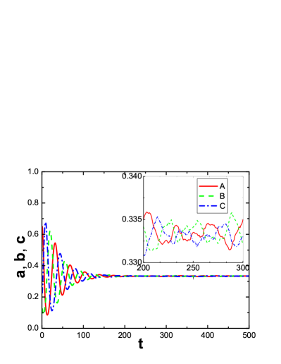
(a)

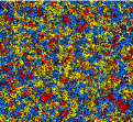
(b)

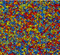
(c)

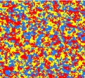
(d)

Figure 1: (Color online.) (a) Temporal evolution for the population densities of species $A$ (red/solid line), $B$(green/dashed), and $C$ (blue/dash-dotted) with symmetric reaction rates $k_{a}=k_{b}=k_{c}=0.5$ and without site occupation restriction (model 1), with unequal initial densities $a(0)=2/3$, $b(0)=c(0)=1/6$, averaged over 50 Monte Carlo runs on a 256 $\times$ 256 square lattice. (b) Snapshot of the spatial particle distribution for a single simulation run at $t=50$, and (c) at $t=500$ MCS; (d): snapshot at $t=500$ MCS, for a system where at most one particle of either species is allowed per site (model 2). (Color coding shows the majority species on each site; red/gray: species $A$, yellow/light gray: $B$, blue/dark gray: $C$, black: empty site.)

We first report and discuss our Monte Carlo simulation results on a 256 $\times$ 256 square lattice with periodic boundary conditions. The data are typically averaged over 50 Monte Carlo runs with different initial configurations, where the particles of each species are placed randomly on the lattice. Figure 1a depicts the temporal evolution of the total population densities in a system without site occupation number restrictions and with equal reaction rates $k_{a}=k_{b}=k_{c}=0.5$ (labeled model 1 in Table 1), but unequal initial densities $a(0)=2/3$, $b(0)=c(0)=1/6$, along with two snapshots 1b,1c of their spatial distribution at different times. Since the selection and reproduction processes are combined into a single step in our model, the total population density $\rho$ is strictly conserved, and as expected we therefore observe no spiral patterns that are characteristic of RPS models without conservation law Matti . In the initial time regime, we see distinct decaying population oscillations in Fig. 1a, and inhomogeneous species clusters in the snapshot Fig. 1b. As time progresses, the amplitude of the oscillating fluctuations decreases quickly, and also the spatial distribution and species cluster size become more stable and homogeneous (Fig. 1c). Our (fairly large) system eventually settles in a coexistence state with small density fluctuations (Fig. 1a inset). For comparison, Fig. 1d shows a snapshot in a system with identical reaction rates and asymmetric initial densities, but with all site occupation numbers restricted to at most a single particle (model 2); one observes the same small cluster structure as in the absence of occupation restrictions.

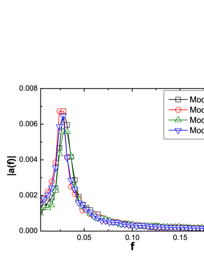
Figure 2: (Color online). Signal Fourier transform $|a(f)|$ of species $A$ density data on a 256 $\times$ 256 square lattice with initial population densities $a(0)=b(0)=c(0)=1/3$ for the four model variants described in Table 1, averaged over 50 Monte Carlo simulation runs.

In Fig. 2 we show the absolute values of the Fourier transformed population density signals $|a(f)|$, as obtained from averaging 50 Monte Carlo simulation runs for the four different model variants listed in Table 1, in this case with equal initial densities $a(0)=b(0)=c(0)=1/3$. Recall that mean-field theory predicts a regular, undamped oscillation frequency $f\approx 0.046$. From the simulation data, we determine the characteristic peak frequency $f\approx 0.028$, which evidently governs oscillatory fluctuations; however, the finite width of the Fourier peak in Fig. 2 reflects that the population oscillations are damped and will cease after a finite characteristic relaxation time.

Moreover, we see that even if spatial disorder and/or site occupancy restrictions are incorporated in the model, the Fourier-transformed density signals display practically the same frequency distribution and significant peak locations. Indeed, we find that in our simulations for model versions 1 and 3 with total density $1$, the typical occupation number at each site remains $n\leq 2$ throughout the runs, which explains why the exclusion constraints in model variants 2 and 4 do not have a large effect. Thus, neither spatial disorder nor site occupancy restrictions change the temporal evolution pattern of the system markedly. This is in stark contrast with results for the two-species stochastic lattice Lotka–Volterra model, for which one finds (i) very pronounced spatio-temporal structures in the species coexistence regime Ivan ; (ii) large fluctuations that strongly renormalize the characteristic population oscillation frequency Ivan ; Mark ; (iii) an extinction threshold for the predator species induced by local density restrictions on the prey Ivan ; and (iv) considerable enhancement of the asymptotic densities of both species caused by spatial variability of the predation rate Ulrich .

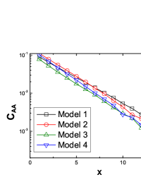
(a)

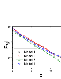
(b)

Figure 3: (Color online.) (a) Static density autocorrelation function $C_{AA}(x)$ and (b) cross-correlation function $C_{AB}(x)$ (linear-$log_{10}$ plots) measured at $t=250$ MCS for the four model variants described in Table 1, with initial population densities $a(0)=b(0)=c(0)=1/3$.

	Model 1	Model 2	Model 3	Model 4
$l_{AA}$	3.27 $\pm$ 0.02	2.92 $\pm$ 0.02	2.64 $\pm$ 0.03	2.59 $\pm$ 0.01
$l_{AB}$	2.86 $\pm$ 0.08	2.35 $\pm$ 0.09	2.40 $\pm$ 0.06	1.99 $\pm$ 0.09

Table 2: Correlation lengths $l_{AA}$ for the autocorrelation function and $l_{AB}$ for the cross-correlation function (in units of the lattice spacing) obtained for the four model variants of Table 1 with symmetric reaction rates.

In order to study the effect of spatial disorder and site occupation restriction on emerging correlations in our stochastic RPS models, we have determined the equal-time two-point correlation functions in the quasi-stationary (long-lived) coexistence state illustrated for models 1 and 2 in Figs. 1c and 1d, respectively. These static correlation functions can quantitatively capture the emerging spatial structures in the lattice. Figures 3a and 3b depict the autocorrelation function $C_{AA}(x)$ and the cross-correlation function $C_{AB}(x)$ as obtained for our four models (see Table 1), which all are seen to decay exponentially with distance, i.e., $C_{AA}(x)\propto e^{-|x|/l_{AA}}$ and $C_{AB}(x)\propto e^{-|x|/l_{AB}}$. From these log-normal plots, we have extracted the associated correlation length $l_{AA}$ and typical species separation distance $l_{AB}$; the results are listed in Table 2. It is worth noticing that in systems exhibiting spiralling patterns, as in the four-state RPS model without conservation law, the correlation functions $C_{AA}(x)$ and $C_{AB}(x)$ do not fall off exponentially but exhibit (damped) oscillations, see e.g. Refs. Reichenbach3 ; Reichenbach4 . Site occupation restrictions clearly have the effect of reducing both correlation lengths. Also, as is the case for the two-species lattice Lotka–Volterra system Ulrich , rendering the reaction rate a quenched random variable for each site leads to more localized population and activity patches, characterized by markedly smaller correlation and typical separation lengths.

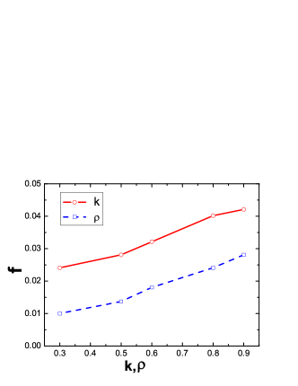
Figure 4: (Color online.) Variation of the characteristic peak frequency in the density Fourier signal $|a(f)|$ with the total density $\rho$ and homogeneous, symmetric reaction rate $k$, for RPS simulations on a 256 $\times$ 256 square lattice with equal initial densities, run for 1000 MCS.

The influence of varying (homogeneous and symmetric) reaction rates and modifying the total (conserved) population density is explored in Fig. 4, which shows the dependence of the characteristic Fourier peak frequency $f$ on $k$ and $\rho$. We find that $f$ scales roughly linearly with both the total density $\rho$ and the reaction rate $k$, in accord with the mean-field prediction $f\propto\rho\,k$, see Sec. II. We have also checked that switching off nearest-neighbor hopping (setting $D=0$), thus allowing particle spreading only via the nonlinear reaction processes (1), essentially leaves the stochastic RPS system’s features intact.

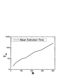
(a)

(b)

Figure 5: (a) Mean extinction time as function of lattice size $N$ (linear-$log_{10}$ plot), obtained from averages over 50 Monte Carlo runs, for small two-dimensional lattice RPS systems in the absence of site restrictions and with symmetric reaction rates $k_{a}=k_{b}=k_{c}=0.5$ (model 1), and equal initial population densities $a(0)=b(0)=c(0)=1/3$. The data are for lattices with $N=5\times 5$, $7\times 7$, $10\times 10$, $12\times 12$, $15\times 15$, $17\times 17$, and $20\times 20$ sites. (b) Histogram of measured extinction times for $N=100$ sites.

Finally, we have also studied the mean extinction time as function of lattice size $N$ for small two-dimensional stochastic lattice RPS systems, here of the model 1 variety with homogeneous symmetric reaction rates $k_{a}=k_{b}=k_{c}=0.5$ and equal initial densities $a(0)=b(0)=c(0)=1/3$. We recall that in any finite system displaying an absorbing stationary state, stochastic fluctuations will eventually reach this absorbing configuration. In the stochastic RPS model, one therefore expects two species to eventually become extinct; however, reaching this absorbing state may take an enormous amount of time, and will thus become practially unobservable on large lattices. In fact, in two and higher dimensions one expects the mean extinction time $T_{\rm ex}$ (here measured for the first species to die out) to scale exponentially with system size $N$, since random fluctuations effectively have to overcome a finite barrier in order to follow an ‘optimal’ path towards extinction. As depicted in Fig. 5a, we indeed observe $\ln T_{\rm ex}(N)\sim N$, consistent with the prediction on the coexistence state stability reported in Refs. Reichenbach1 ; Reichenbach4 . The associated distributions of extinction times are described by neither Poisson nor Gaussian distributions (e.g., the means are considerably larger than the most likely values), but display long ‘fat’ tails at large extinction times, see Fig. 5b. We expect similar features in model variant 2, in accord with the remarkably long-live species coexistence observed in Ref. Tainaka1 .

III.3 Two-dimensional stochastic RPS system: asymmetric rates

Model	Reaction rates	Site restriction
1	$k_{a}=0.2,k_{b}=0.5,k_{c}=0.8$	no restriction
2	$k_{a}=0.2,k_{b}=0.5,k_{c}=0.8$	at most one
3	$k_{a}\in[0,0.4]$, $k_{b}=0.5$, $k_{c}=0.8$	no restriction
4	$k_{a}\in[0,0.4]$, $k_{b}=0.5$, $k_{c}=0.8$	at most one

Table 3: List of stochastic lattice RPS model variants with asymmetric rates. While $k_{b}=0.5$ and $k_{c}=0.8$ are held fixed in all four variants, we set $k_{a}=0.2$ in models 1 and 2, whereas we took $k_{a}$ to be a random variable uniformly distributed in $[0,0.4]$ in models 3 and 4.

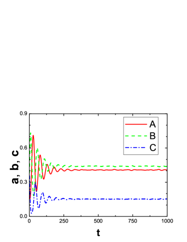
(a)

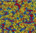
(b)

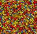
(c)

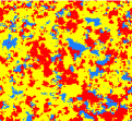
(d)

Figure 6: (Color online.) (a) Temporal evolution for the population densities of species $A$ (red/solid line), $B$ (green/dashed), and $C$ (blue/dash-dotted) with asymmetric reaction rates $k_{a}=0.2$, $k_{b}=0.5$, $k_{c}=0.8$ and without site occupation restriction (model 1), with equal initial densities $a(0)=b(0)=c(0)=1/3$, averaged over 50 runs on a 256 $\times$ 256 square lattice. (b) Snapshot of the spatial particle distribution in a single simulation run at $t=50$, and (c) at $t=500$ MCS; (d): snapshot at $t=500$ MCS, for a system where at most one particle of either species is allowed per site (model 2). (Majority species coloring: red/gray: $A$, yellow/light gray: $B$, blue/dark gray: $C$, black: empty.)

Next we turn to a stochastic RPS system with asymmetric reaction rates and consider the various model variants specified in Table 3 together with the reactions (1). Figure 6a shows the time evolution for the three species’ densities in a system with constant rates $k_{a}=0.2$, $k_{b}=0.5$, and $k_{c}=0.8$. From our simulations for model version 1, we infer the asymptotic population densities (with statistical errors) $(0.40\pm 0.01,0.45\pm 0.01,0.15\pm 0.01)$, which follow the trends of the mean-field results $(a^{*},b^{*},c^{*})=(0.33,0.53,0.13)$. As becomes apparent in the snapshots 6b and 6c for model variant 1 without site restrictions, and 6d for a system with at most a single particle per site (model 2), particles of the same species form distinctive spatial clusters. The effect of the reaction rate asymmetry on the equal-time auto- and cross-correlation functions is shown in Figs. 7a and 7b, respectively, with the ensuing correlation lengths and typical separation distances listed in Table 4. Note that the autocorrelation length $l_{CC}$ for species $C$ is smaller than $l_{AA}$, and $l_{BB}$, which is largest. This is consistent with the long-time densities in the (quasi-stationary) coexistence state, given our observation that the overall particle density is roughly uniform.

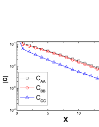
(a)

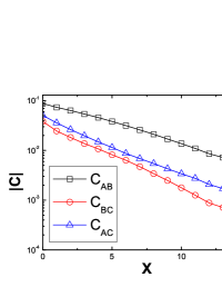
(b)

Figure 7: (Color online.) (a) Equal-time autocorrelation functions $C_{AA}(x)$, $C_{BB}(x)$, $C_{CC}(x)$ at $t=1000$ MCS for the model described in Fig. 6. (b) Equal-time cross-correlation functions $C_{AB}(x)$, $C_{BC}(x)$, $C_{AC}(x)$ (linear-$log_{10}$ plots).

$l_{AA}$	$l_{BB}$	$l_{CC}$
5.24 $\pm$ 0.03	5.67 $\pm$ 0.08	3.46$\pm$0.05
$l_{AB}$	$l_{BC}$	$l_{AC}$
6.68 $\pm$ 0.20	3.68 $\pm$ 0.07	3.33 $\pm$ 0.05

Table 4: Correlation lengths (top) inferred from the autocorrelation functions and typical separation distances (bottom) obtained from the cross-correlation functions (in units of the lattice spacing) measured for the RPS model with asymmetric but homogeneous reaction rates $k_{a}=0.2$, $k_{b}=0.5$, and $k_{c}=0.8$.

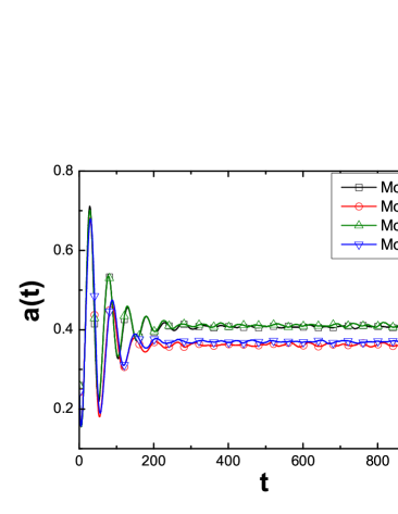
Figure 8: (Color online.) Time evolution for the population density $a(t)$ of species $A$ for four model variants with asymmetric reaction rates, namely with $k_{b}=0.5$, $k_{c}=0.8$ and either uniformly $k_{a}=0.2$, or drawn from a flat distribution $[0,0.4]$, with and without site restrictions (see the listing in Table 3). The initial densities are $a(0)=b(0)=c(0)=1/3$, and the data stem from averages over 50 runs on a 256 $\times$ 256 square lattice.

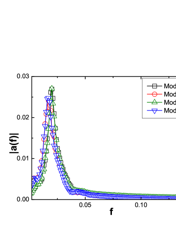
Figure 9: (Color online.) Signal Fourier transform $|a(f)|$ for the four model variants described in Table 3. The characteristic frequency comes out to be $f\approx 0.021$.

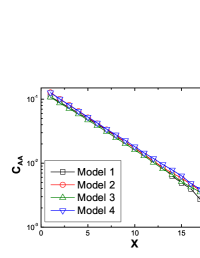
(a)

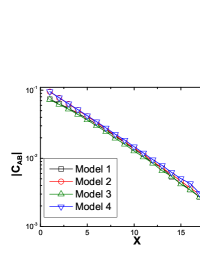
(b)

Figure 10: (Color online.) (a) Equal-time autocorrelation function $C_{AA}(x)$ and (b) cross-correlation functions $C_{AB}(x)$ (linear-$log_{10}$ plots) at $t=1000$ MCS for the four model variants described in Table 3.

As a last model variation, we allow the reaction rate $k_{a}$ to be a quenched spatial random variable drawn from the flat distribution $[0,0.4]$, such that its average is still $0.2$, but hold $k_{b}=0.5$ and $k_{c}=0.8$ fixed. Fig. 8 compares the time evolution for these disordered systems with and without site restrictions with the corresponding homogeneous models. Once again, we see that spatial variability in the reaction rate even in this asymmetric setting has very little effect. As can be seen from the Fourier signal peak in Fig. 9, the characteristic frequency comes out to be $f\approx 0.021$ for all four asymmetric model variants investigated here, and Figs. 10a and 10b demonstrate that the disorder hardly modifies the spatial decay of the auto- and cross-correlation functions either.

III.4 One-dimensional Monte Carlo simulations

We have run simulations for all four model variants listed in Table 1, i.e., with/without site occupancy restriction; with/without quenched spatial randomness in the reaction rates, in one dimension. We find that only a single species ultimately survives and eventually occupies the whole lattice no matter whether spatial disorder or site restrictions are included in the model: as expected, the one-dimensional system will always evolve towards one of the three extinction states where two of the three species will die out. While this phenomenon also occurs in two dimensions, in $d=1$ the species coexist over a time that on average scales polynomially with the system size (see below), i.e., extinction happens on a much shorter time scale than in two dimensions (see Fig. 5a). Again, for equal (mean) reaction rates and initial densities, each species has equal survival probability. For comparison, the space-time plots of one-dimensional lattice simulations without and with site occupancy restriction are depicted in Figs. 11 and 12, respectively. It is seen that individuals of identical species cluster together, and any reactions are confined to the boundary separating the single-species domains. When the occupancy of any site is restricted to a single particle of either species, these domains form quickly and are very robust, even if not all sites are filled, see Figs. 12a and 12b.

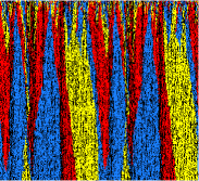
Figure 11: (Color online.) Time evolution (up to 1000 Monte Carlo steps; from top to bottom) for a one-dimensional RPS model run with equal, homogeneous reaction rates $k_{a}=k_{b}=k_{c}=0.5$, equal initial densities $a(0)=b(0)=c(0)=1/3$, and in the absence of site occupancy restriction. (Only 10000 of the total 50000 lattice sites in this run are shown; majority species coloring in red/gray: $A$, yellow/light gray: $B$, blue/dark gray: $C$, black: empty.)

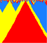
(a)

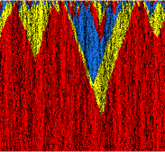
(b)

Figure 12: (Color online.) Time evolution (up to 1000 Monte Carlo steps; from top to bottom) for one-dimensional RPS model runs with equal, homogeneous reaction rates $k_{a}=k_{b}=k_{c}=0.5$, equal initial densities (a) model 2: $a(0)=b(0)=c(0)=1/3$, and (b) model 2’: $a(0)=b(0)=c(0)=0.2$ (model 2’ and 4’ refer to the corresponding model variants listed in Table 1 with total particle density less than $1$), where at most one particle of either species is allowed per site. (Only 10000 of the total 50000 lattice sites in these runs are shown; red/gray: $A$, yellow/light gray: $B$, blue/dark gray: $C$, black: empty.)

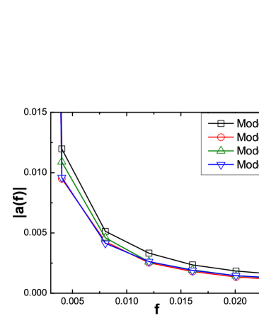
Figure 13: (Color online.) Signal Fourier transform $|a(f)|$ for the four RPS model variants listed in Table 1, in one dimension. The data is averaged over 50 Monte Carlo simulations on lattices with 50000 sites.

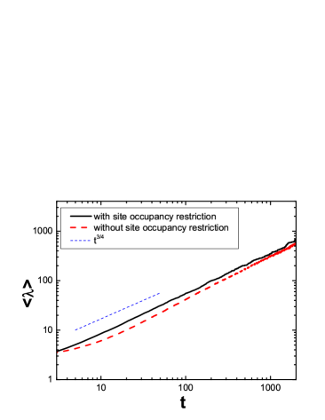
Figure 14: (Color online.) The time evolution ($log_{10}-log_{10}$ plot) of the mean single-species domain size $\langle\lambda(t)\rangle$ measured in one-dimensional Monte Carlo simulation runs with 10000 lattice sites for RPS models with symmetric reaction rates $k_{a}=k_{b}=k_{c}=0.5$ and equal initial densities $a(0)=b(0)=c(0)=1/3$. The upper (black) curve shows the data for model 2 with site occupation restriction, see Fig. 12a, whereas the lower (red/dashed) graph pertains to model variant 1 without site occupancy restrictions, see Fig. 11. For comparison, the blue/dotted straight line represents the predicted $t^{3/4}$ power law.

The population density signal Fourier transform $|a(f)|$, shown for species $A$ in Fig. 13, confirms the absence of any population oscillations through the absence of any peak at nonzero frequency $f$, and the width of the peak at $f=0$ reflects the decay time to the stationary extinction state. As in two dimensions, we observe very little effect of either site occupation number restrictions or spatial variability of the reaction rates on the Fourier signal, compare Figs. 2 and 9. We have also measured the mean single-species domain size $\langle\lambda(t)\rangle$ and investigated its growth with time $t$, shown in Fig. 14. As was predicted in Refs. Frache1 ; Frache2 , for the implementation with site occupancy restriction (model 2) to at most a single particle per site, we observe $\langle\lambda(t)\rangle\sim t^{3/4}$; we find the same asymptotic growth law when arbitrarily many particles are allowed on each lattice site. An algebraic decay of the number of domains was also reported in Ref. Tainaka1 . The domain stability is further illustrated by the very slow temporal decay of the on-site auto- and cross-correlation functions (see Figs. 15a and 15b). Notice that quenched spatial disorder in the reaction rates does not affect the time evolution of the autocorrelation functions, in contrast with site occupancy restrictions; here the results depend on the presence or absence of empty sites, see Fig. 15a. However, the cross-correlation functions in Fig. 15b look essentially indistinguishable for all these model variations.

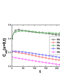
(a)

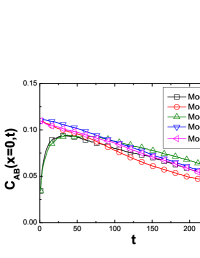
(b)

Figure 15: (Color online.) Time evolution for the on-site (a) autocorrelation $C_{AA}(0,t)$ and (b) cross-correlation function $C_{AB}(0,t)$ in one-dimensional RPS model variants with 500 sites, averaged over 1000 simulation runs. Shown are the results for model variants 1–4 with initial densities $a(0)=b(0)=c(0)=1/3$; model 2’ refers to a system with site occupancy restriction 1 and lower particle density $a(0)=b(0)=c(0)=1/4$.

Figures 16a and 16b respectively depict the equal-time auto- and cross-correlation functions for the various model variants listed in Table 1 obtained for a one-dimensional lattice with 50000 sites. We observe exponential decay with similar large correlation lengths for all model variants upto about 50 lattice sites, followed by a cutoff (which extends to larger $x$ as time increases).

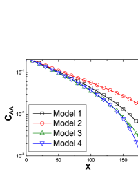
(a)

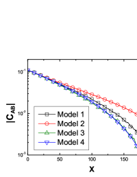
(b)

Figure 16: (Color online.) (a) Static autocorrelation functions $C_{AA}(x)$ and (b) static cross-correlation functions $C_{AB}(x)$ (linear-$log_{10}$ plots) measured at $t=250$ MCS for the four RPS model variants described in Table 1 on a one-dimensional lattice with 50000 sites, averaged over 50 simulation runs.

Finally, we investigate the mean extinction time as function of system size $N$ in one dimension. As becomes apparent in Figs. 17a, in all one-dimensional model variants we have considered, within our (large) error bars the mean extinction time appears to follow a power law $T_{\rm ex}\sim N^{\gamma}$, as proposed in Refs. Schutt ; Reichen ; Dobrienski ; Parker . However, a best power-law fit yields variable effective exponents $T_{\rm ex}\sim N^{\gamma}$ with $\gamma$ ranging from $\sim 1.5$ to $\sim 1.8$ if we fit the data up to $N=50$ or $N=200$, respectively, rather than $\gamma=2$ Schutt or $\gamma=1$ Reichen ; Dobrienski ; Parker . Biasing the data towards smaller systems for which the statistical errors are likely better controlled, our results may even be consistent with the mean-field value $\gamma=1$. Note, however, that the extinction time distribution acquires even fatter tails at large times than in two dimensions, see Fig. 17b, and rare long survival events dominate the averages and induce large statistical fluctuations. The mean extinction time alone therefore poorly characterizes the extinction kinetics. When the reaction rates are chosen asymmetric, we have checked that only the ‘weakest’ species with the smallest predation rate survives, whereas the other two species are driven to extinction Frean ; Berr .

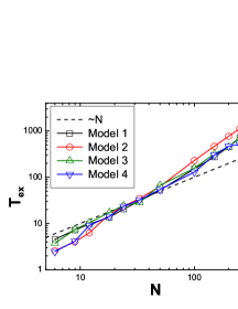
(a)

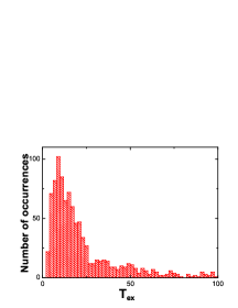
(b)

Figure 17: (Color online.) (a) Mean extinction time as function of lattice size $N$ ($log_{10}-log_{10}$ plot), obtained from averages over 1000 Monte Carlo runs, in one dimension. (b) Histogram of the measured extinction times for model variant 2 with $N=30$; compare with Figs. 5a and 5b.

IV Conclusion

In this paper, we have studied the effects of finite carrying capacity and spatial variability in the reaction rates on the dynamics of a class of spatial rock–paper–scissors (RPS) models. We have investigated the properties of several variants of the stochastic four-state zero-sum RPS game (with conserved total particle number) on two- and one-dimensional lattices with periodic boundary conditions. In two dimensions, owing to the strict (local) conservation of the total particle number, one does not observe the formation of spiral patterns; the three species simply form small clusters. In fact, spatial correlations are weak in the (quasi-stationary) coexistence state, and the system is remarkably well described by the mean-field rate equation approximation. Typical extinction times scale exponentially with system size Reichenbach4 , resulting in coexistence of all three species already on moderately large lattices. We find the characteristic initial oscillation frequency to be proportional to the reaction rate and total particle density, as predicted by mean-field theory.

We observe that neither site occupation number restrictions nor quenched spatial disorder in the reaction rates markedly modify the populations’ temporal evolution, species density Fourier signals, or equal-time spatial correlation functions. This observation holds for models with symmetric as well as asymmetric reaction rates, and even if spatial variability is introduced only for the competition of one species pair. On the basis of the mean-field results, this very weak disorder effect is a consequence of the essentially linear dependence of the long-time densities on the reaction rates $k$; averaging over a symmetric distribution just yields the average. In the two-species Lotka–Volterra model, instead both the asymptotic predator and prey densities are inversely proportional to the predation rate, and averaging over a distribution of the latter strongly biases towards small rate values and large densities Ulrich . Both in the two- and cyclic three-species systems, spatially variable rates induce stronger localization of the species clusters.

In one dimension, two species are driven towards extinction with the mean extinction time $T_{\rm ex}\sim N^{\gamma}$, $\gamma\approx 1\ldots 1.8$ (with large error bars), and only a single species survives. The distribution of extinction times displays fat long-time tails. We confirm that the single-species domains grow with the predicted power law $\langle\lambda(t)\rangle\sim t^{3/4}$ in the models with site restrictions Frache1 ; Frache2 , and we have obtained similar results for the model variants with an infinite carrying capacity. For asymmetric reaction rates, we have also checked that the ‘weakest’ species is the surviving one Frean ; Berr .

Our results demonstrate that the physical properties of cyclic RPS models are quite robust, even quantitatively, with respect to modifications of their ‘microscopic’ model definitions and characterization. This is in stark contrast with the related two-species Lotka–Volterra predator-prey interaction model. We believe the origin of this remarkable robustness lies in the comparatively weaker prominence of stochastic fluctuations and spatial correlations in the cyclic three-species system. The robustness of the RPS models considered here implies that environmental noise can be safely ignored and that their properties are essentially independent of the carrying capacity. It is worth emphasizing that this result is nontrivial; in terms of modeling such systems, it notably implies that one has the freedom to consider strict site restriction ($n_{m}=1$) and hence simplify the numerical calculations, or to set $n_{m}=\infty$ (no site restrictions) and thus facilitate the mathematical treatment. In fact, our study establishes that both ‘microscopic’ model realizations are essentially equivalent. As it turns out, this conclusion also pertains to spatial May–Leonard models MayLeonard ; DurrettLevin , as we shall report in detail elsewhere HMT .

- (1) R. M. May, Stability and Complexity in Model Ecosystems (Cambridge University Press, Cambridge, 1974).
- (2) J. Maynard Smith, Models in Ecology (Cambridge University Press, Cambridge, 1974).
- (3) R. E. Michod, Darwinian Dynamics (Princeton University Press, Princeton, 2000).
- (4) R. V. Sole and J. Basecompte, Self-Organization in Complex Ecosystems (Princeton University Press, Princeton, 2006).
- (5) D. Neal, Introduction to Population Biology (Cambridge University Press, Cambridge, 2004).
- (6) A. J. Lotka, J. Amer. Chem. Soc. 42, 1595 (1920).
- (7) V. Volterra, Mem. Accad. Lincei. 2, 31 (1926).
- (8) J. Maynard Smith, Evolution and the Theory of Games (Cambridge University Press, Cambridge, 1982).
- (9) J. Hofbauer and K. Sigmund, Evolutionary games and population dynamics (Cambridge University Press, Cambridge, 1998).
- (10) R. M. Nowak, Evolutionary Dynamics (Belknap Press, Cambridge(USA), 2006).
- (11) G. Szabó and G. Fáth, Evolutionary games on graphs, Phys. Rep. 446, 97 (2007).
- (12) D. Volovik, M. Mobilia, and S. Redner, Eur. Phys. Lett. 85, 480003 (2009).
- (13) M. Mobilia, J. Theor. Biol. 264, 1 (2010).
- (14) B. Sinervo and C.M. Lively, Nature 380, 240 (1996).
- (15) K. R. Zamudio and B. Sinervo, Proc. Natl. Acad. Sci. U.S.A. 97, 14427 (2000).
- (16) B. Kerr, M. A. Riley, M. W. Feldman, and B. J. M. Bohannan, Nature 418, 171 (2002).
- (17) J. B. C. Jackson and L. W. Buss, Proc. Nat. Acad. Sci. U.S.A. 72, 516 (1975); Am. Nat. 113, 223 (1979).
- (18) L. W. Buss, Proc. Nat. Acad. Sci. U.S.A. 77, 5355 (1980).
- (19) M. T. Burrows and S. J. Hawkins, Mar. Ecol. Prog. Ser. 167, 1 (1998).
- (20) M. Ifti and B. Bergersen, Eur. Phys. J. E 10, 241 (2003).
- (21) T. Reichenbach, M. Mobilia, and E. Frey, Phys. Rev. E. 74, 051907 (2006).
- (22) M. Frean and E. R. Abraham, Proc. R. Soc. Lond. B 268, 1323 (2001).
- (23) M. Berr, T. Reichenbach, M. Schottenloher, and E. Frey, Phys. Rev. Lett. 102, 048102 (2009).
- (24) K. I. Tainaka, J. Phys. Soc. Jpn. 57, 2588 (1988).
- (25) L. Frachebourg, P. L. Krapivsky, and E. Ben-Naim, Phys. Rev. Lett. 77, 2125 (1996).
- (26) L. Frachebourg, P. L. Krapivsky, and E. Ben-Naim, Phys. Rev. E. 54, 6186 (1996).
- (27) A. Provata, G. Nicolis, and F. Baras, J. Chem. Phys. 110, 8361 (1999).
- (28) S. Venkat and M. Pleimling, Phys. Rev. E 81, 021917 (2010).
- (29) K. I. Tainaka, Phys. Lett. A 176, 303 (1993).
- (30) K. I. Tainaka, Phys. Rev. E 50, 3401 (1994).
- (31) G. Szabó and A. Szolnoki, Phys. Rev. E 65, 036115 (2002).
- (32) M. Perc, A. Szolnoki and G. Szabo, Phys. Rev. E 75, 052102 (2007).
- (33) T. Reichenbach, M. Mobilia, and E. Frey, Nature 448, 1046 (2007).
- (34) T. Reichenbach, M. Mobilia, and E. Frey, Phys. Rev. Lett. 99, 238105 (2007).
- (35) T. Reichenbach, M. Mobilia, and E. Frey, Banach Center Publications Vol.80, 259 (2008).
- (36) T. Reichenbach, M. Mobilia, and E. Frey, J. Theor. Biol. 254, 368 (2008).
- (37) G. A. Tsekouras and A. Provata, Phys. Rev. E. 65, 016204 (2001).
- (38) M. Peltomäki and M. Alava, Phys. Rev. E. 78, 031906 (2008).
- (39) A. Dobrienski and E. Frey, e-print arXiv:1001.5235.
- (40) M. Mobilia, I. T. Georgiev, and U. C. Täuber, J. Stat. Phys. 128, 447 (2007); and references therein.
- (41) M. J. Washenberger, M. Mobilia, and U. C. Täuber, J. Phys.: Condens. Matter. 19, 065139 (2007).
- (42) U. Dobramysl and U. C. Täuber, Phys. Rev. Lett. 101, 258102 (2008).
- (43) S. P. Hubbell, The Unified Neutral Theory of Biodiversity and Biogeography (Princeton University Press, Princeton, 2001).
- (44) I. A. Hanski and O. E. Gagiotti (Eds.), Ecology, genetics, and evolution of metapopulations (Elsevier Academic Press, 2004).
- (45) Q. He, M. Mobilia, and U. C. Täuber, in preparation.
- (46) R. M. May and W. Leonard, SIAM J. Appl. Math. 29, 243 (1975).
- (47) R. Durrett and S. Levin, J. Theor. Biol. 185, 165 (1997); Theor. Pop. Biol. 53, 30 (1998).
- (48) M. Schütt and J.C. Claussen, e-print arXiv:1003.2427.
- (49) M. Parker and A. Kamenev, Phys. Rev. E 80, 021129 (2009).