Coupled tensorial form for atomic relativistic two-particle operator given in second quantization representation

Abstract

General formulas of the two-electron operator representing either atomic or effective interactions are given in a coupled tensorial form in relativistic approximation. The alternatives of using uncoupled, coupled and antisymmetric two-electron wave functions in constructing coupled tensorial form of the operator are studied. The second quantization technique is used. The considered operator acts in the space of states of open-subshell atoms.

Rytis Juršėnas, Gintaras Merkelis

Institute of Theoretical Physics and Astronomy of Vilnius University,
A. Goštauto 12, LT-01108 Vilnius, Lithuania

1 Introduction

In the atomic structure calculations, investigations to optimize the effort of obtaining matrix elements of a two-electron operator are urgently required. This can be explained by the fact that theoretical methods recently used to produce high-precision atomic structure data generate large sets of matrix elements for a two-particle operator. This leads to large computation requirements in terms of both memory and speed. For example, large-scale configuration interaction (CI) calculations [1]-[5] use a massive matrix for the atomic Hamiltonian. A large fraction of expansion terms of perturbation theory (PT) recently applied in atomic calculations [6]-[11] are considered as matrix elements of some effective two-particle operators with complex tensorial structures. In all the above mentioned studies, a significant fraction of computations are devoted to the calculation of $N$-electron angular parts of the matrix elements of a two-electron operator. Particularly complex calculations emerge when more than two open subshells with $N>2$ are involved. A number of methods and techniques [12]-[17] were developed in order to obtain the general formulas for matrix elements of a two-particle operator for many electron case. The comprehensive description of this subject can be found everywhere [12], [19].

In the present paper we distinguish the second quantization representation (SQR) [8], [13], [14]. The efficiency of this technique manifests itself when the tensorial properties of creation and annihilation operators are taken into account [14]. Then the $N$-electron angular part of a matrix element is described by a coupled tensorial product of creation and annihilation operators. In order to optimize (minimize) the calculation procedures it is important to choose the appropriate coupling schemes of angular momenta and the order of creation and annihilation operators in the tensorial product. In [5] and [16] the coupling schemes for the tensorial products of creation and annihilation operators were considered for nonrelativistic ($LS$-coupling) and relativistic ($jj$-coupling) cases, respectively. The manner to determinate the expressions for matrix elements was presented. In [17] a coupled tensorial form of an effective two-particle operator used in a second-order MBPT was obtained in $LS$-coupling. Here, the different forms [16] of coupling schemes to make tensorial product for particular cases were suggested. This enables one to reduce the complexity of the expressions for matrix elements. In [18] the investigations of [17] were extended by including into the presentation of coupled tensorial form of a two-particle operator coupled and antisymmetric two-electron wave functions given in $LS$-coupling.

In the present manuscript we continue the studies of [18] by considering a two-particle operator in $jj$-coupling (in the relativistic approximation [3]). We search for the general expressions of formal (effective) two-particle operator which describes atomic interactions as well as effective interactions in atoms. In Section 2 a coupled form of the two-electron operator is studied using uncoupled, coupled and antisymmetric two-electron wave functions. Sets of expressions for the two-electron operator are given in SQR (see Tables). An example of the application of obtained results for specific cases is considered in Section 3.

2 Coupling schemes of ranks for a two-particle operator

Let us consider a two-particle operator $G$ given in the second quantization representation (SQR) in $jj$-coupling [14]:

$$G=X\displaystyle\sum_{\alpha\beta\mu\nu}a_{\alpha}a_{\beta}a_{\nu}^{\dagger}a_{\mu}^{\dagger}\,\,g(\alpha,\beta,\mu,\nu;\gamma,m_{\gamma}).$$ (1)

In our considerations $\alpha,\beta,\nu,\mu$ indicate the subshells $n_{\alpha}\lambda_{\alpha}m_{\alpha},n_{\beta}\lambda_{\beta}m_{\beta},n_{\nu}\lambda_{\nu}m_{\nu},n_{\mu}\lambda_{\mu}m_{\mu}$ of $N$-electron wave function ${{\left|\Psi^{N}\right\rangle\equiv\left|n_{a}\lambda_{a}^{N_{a}}\Lambda_{a}\,n_{b}\lambda_{b}^{N_{b}}\Lambda_{b}...n_{k}\lambda_{k}^{N_{k}}\Lambda_{k}\,\left(\Lambda_{ab}...\right)\;\Lambda M_{\Lambda}\right\rangle}}$, the operator $G$ acts on. Operators $a_{i}$ and $a_{i}^{\dagger}$ denote electron creation and annihilation operators in the state $n_{i}\lambda_{i}m_{i}$ ($\lambda_{i}=l_{i}j_{i}$, $l_{i}-$parity of the state) with principal quantum number $n_{i}$ and magnetic quantum number (projection) $m_{i}$. In the present paper the factor $g(\alpha,\beta,\mu,\nu;\gamma,m_{\gamma})$ is associated with a matrix element ${\left\langle n_{\alpha}\lambda_{\alpha}m_{\alpha}n_{\beta}\lambda_{\beta}m_{\beta}\left|g_{m_{\gamma}}^{(\gamma)}(1,2)\right|n_{\mu}\lambda_{\mu}m_{\mu}n_{\nu}\lambda_{\nu}m_{\nu}\right\rangle}$ of a two-electron operator

$$G=\displaystyle\sum_{i<j}^{N}g_{ij}=\frac{1}{2}\sum_{i\neq j}\,g_{ij}$$ (2)

of atomic interactions. We assume that $g_{ij}$ can be expressed by the tensorial product [12]:

$$g_{ij}\equiv g_{m_{\gamma}}^{(\gamma)}(i,j)=\displaystyle\sum_{\gamma_{1}\gamma_{2}}g(r_{i},r_{j})g_{m_{\gamma}}^{(\gamma_{1}\,\gamma_{2})(\gamma)}=\displaystyle\sum_{\gamma_{1}\gamma_{2}}g(r_{i},r_{j})\left[g^{(\gamma_{1})}(i)\times g^{(\gamma_{2})}(j)\right]_{m_{\gamma}}^{(\gamma)}$$ (3)

and that $g_{ij}=g_{ji}.$ In (3) $g(r_{i},r_{j})$ is the radial part of $g_{ij}$. An irreducible tensorial operator $g^{(\gamma)}(i)$ acts on the spin-angular variables of the $i$-th electron in the space of one-electron relativistic wave functions ($4$-spinors) [19]

$$\left|n\lambda m\right\rangle\equiv\left|nljm\right\rangle=\left(\begin{array}[]{c}f(nlj|r)\left|ljm\right\rangle\\ (-1)^{\vartheta}g(nl^{\prime}j|r)\left|l^{\prime}jm\right\rangle\end{array}\right),$$ (4)

where $l^{\prime}=2j-l$, $\vartheta=l-j+1/2$. Functions $f(nlj|r)$ and $g(nl^{\prime}j|r)$ are large and small components of $\left|n\lambda m\right\rangle$. Functions $\left|ljm\right\rangle$, $\left|l^{\prime}jm\right\rangle$ are $2$-spinors. In (1) the factor $X=1/2$. However, when $g(\alpha,\beta,\mu,\nu;\gamma,m_{\gamma})$ is associated with the antisymmetric matrix element [10]

$$\left\langle n_{\alpha}\lambda_{\alpha}m_{\alpha}n_{\beta}\lambda_{\beta}m_{\beta}\left|g_{m_{\gamma}}^{(\gamma)}(1,2)\right|n_{\mu}\lambda_{\mu}m_{\mu}n_{\nu}\lambda_{\nu}m_{\nu}\right\rangle_{A}$$

$$=\left[1-\left(\mu\leftrightarrow\nu\right)\right]\left\langle n_{\alpha}\lambda_{\alpha}m_{\alpha}n_{\beta}\lambda_{\beta}m_{\beta}\left|g_{m_{\gamma}}^{(\gamma)}(1,2)\right|n_{\mu}\lambda_{\mu}m_{\mu}n_{\nu}\lambda_{\nu}m_{\nu}\right\rangle,$$ (5)

the factor $X=1/4$. Here $(\mu\leftrightarrow\nu)$ indicates that $\mu$ must be interchanged with $\nu$.

Notice, that when examining the atomic perturbation theory expansion terms or coupled cluster (CC) approach equation ones, they can be considered as the matrix elements of some effective operator ${}^{eff}g_{m_{\gamma}}^{(\gamma)}$ [6]. Then the factor $g(\alpha,\beta,\mu,\nu;\gamma,m_{\gamma})$ can be associated with the matrix element ${\left\langle\alpha\beta\left|{}^{eff}g_{m_{\gamma}}^{(\gamma)}\right|\mu\nu\right\rangle}$. The operator ${}^{eff}g_{m_{\gamma}}^{(\gamma)}$ usually has more complicated tensorial structure and symmetry properties than $g_{m_{\gamma}}^{(\gamma)}$ (3). Nevertheless, the expressions of $G$ developed in this manuscript are also valid for ${}^{eff}g_{m_{\gamma}}^{(\gamma)}$. In the later case the factor $X$ is obtained individually.

Below we briefly describe the procedures that we have used to convert operator $G$ into a coupled tensorial form, i.e., to obtain the expressions for $G$, where the quantities entering these expressions are independent of magnetic quantum numbers $m_{i}$. It is convinient to explain such transformation by examining the schema (Figure 1) which arises when applying a graphical method of angular momentum theory [21]. In schematic form we can write

$$G=X\displaystyle\sum_{\alpha\beta\mu\nu}\,\,\sum_{m_{\alpha}m_{\beta}m_{\mu}m_{\nu}}a_{\alpha}a_{\beta}a_{\nu}^{\dagger}a_{\mu}^{\dagger}\,A_{1}=\sum_{\alpha\beta\mu\nu}\,\sum_{J_{1}J_{2}}\ A_{2}\,\sum_{ud}\,A_{3}\,\ A_{4},$$ (6)

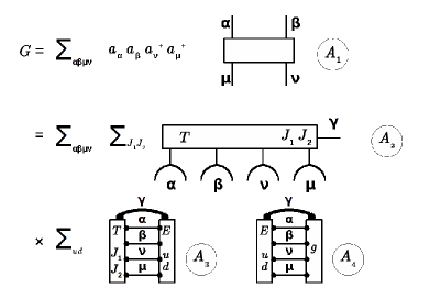
Figure 1: The block-scheme of transforming two-electron operator into coupled tensorial form.

where summation indices $\alpha\beta\mu\nu$ denote quantum numbers $n\lambda$. The diagram $A_{1}$ denotes either a matrix element ${\left\langle\alpha\beta\left|g_{m_{\gamma}}^{(\gamma)}\right|\mu\nu\right\rangle}$ or ${\left\langle\alpha\beta\left|{}^{eff}g_{m_{\gamma}}^{(\gamma)}\right|\mu\nu\right\rangle}$. The irreducible tensorial product (the diagram $A_{2}$) composed of creation and annihilation operators was produced by using Jucys theorems of graphical angular momentum theory [21]. To obtain the desired form of the irreducible product, we carried out several recouplings of angular momenta and made several changes of positions of creation and annihilation operators in (1). The arrangements of operators will be discussed later. Firstly, we shall discuss the recoupling of angular momenta. In this manuscript we investigate two approaches. In each approach the specific coupling schemes of the angular momenta $j$ were applied. The block $E$ of diagrams $A_{3}$, $A_{4}$ represents such schemes. In the first approach we have used the following coupling of momenta

$$E_{b}:=\left[\begin{array}[]{ccc}j_{\mu}&u&j_{\alpha}\\ m_{\mu}&m_{u}&m_{\alpha}\end{array}\right]\left[\begin{array}[]{ccc}j_{\nu}&d&j_{\beta}\\ m_{\nu}&m_{d}&m_{\beta}\end{array}\right]\left[\begin{array}[]{ccc}u&d&\gamma\\ m_{u}&m_{d}&m_{\gamma}\end{array}\right],$$ (7)

while in the second approach, the block $E$ is given by

$$E_{z}:=\left[\begin{array}[]{ccc}j_{\alpha}&j_{\beta}&u\\ m_{\alpha}&m_{\beta}&m_{u}\end{array}\right]\left[\begin{array}[]{ccc}j_{\mu}&j_{\nu}&d\\ m_{\mu}&m_{\nu}&m_{d}\end{array}\right]\left[\begin{array}[]{ccc}u&d&\gamma\\ m_{u}&m_{d}&m_{\gamma}\end{array}\right].$$ (8)

Here $\left[...\right]$ brackets define Clebsch-Gordan coefficients; $u$ and $d$ are the intermediate momenta arising in the recoupling procedure. The block $T$ in $A_{2}$, $A_{3}$ describes the coupling schema of the irreducible tensorial product of creation and annihilation operators with the intermediate ranks $J_{1}$, $J_{2}$. The diagram $A_{3}$ represents the recoupling coefficient of angular momenta $j_{i}$ transforming the schema $E$ into $T$. In the case of (3), due to the chosen specific coupling $E_{b}$, in the first approach the diagram $A_{4}$ corresponds to product of the submatrix element $\left[\lambda_{\alpha}\lambda_{\beta}\left\|g^{(\gamma)}\right\|\lambda_{\mu}\lambda_{\nu}\right]$ and $\delta(u,\gamma_{1})\delta(d,\gamma_{2})$. However, in the second approach $A_{4}$ is associated with submatrix element

$$\left[\lambda_{\alpha}\lambda_{\beta}u\left\|g^{(\gamma)}(1,2)\right\|\lambda_{\mu}\lambda_{\nu}d\right]\\ ={\displaystyle\sum_{\gamma_{1}\gamma_{2}}}\left[j_{\alpha},j_{\beta},\gamma,d\right]^{1/2}\left\{\begin{array}[]{ccc}j_{\mu}&j_{\nu}&d\\ \gamma_{1}&\gamma_{2}&\gamma\\ j_{\alpha}&j_{\beta}&u\end{array}\right\}\left[\lambda_{\alpha}\lambda_{\beta}\left\|g^{(\gamma_{1}\gamma_{2})}\right\|\lambda_{\mu}\lambda_{\nu}\right]R_{\alpha\beta\mu\nu}(1,2).$$ (9)

Here $R_{\alpha\beta\mu\nu}(1,2)$ is a radial integral of a radial function $g(r_{1},r_{2})$ in the basis of $|nlj)$ functions. In (9) the coupled two-electron wave functions

$$\left|n_{i}\lambda_{i}n_{j}\lambda_{j}um_{u}\right\rangle=\displaystyle\sum_{{\scriptstyle m_{\lambda_{i}}m_{\lambda_{j}}}}\left[\begin{array}[]{ccc}\lambda_{i}&\lambda_{j}&u\\ m_{\lambda_{i}}&m_{\lambda_{j}}&m_{u}\end{array}\right]\left|n_{i}\lambda_{i}m_{i}n_{j}\lambda_{j}m_{\lambda_{j}}\right\rangle$$ (10)

are used to determine the matrix element of $g_{m_{\gamma}}^{(\gamma)}$. Note that in the first approach (7) uncoupled wave functions $\left|n_{\alpha}\lambda_{\alpha}m_{\alpha}n_{\beta}\lambda_{\beta}m_{\beta}\right\rangle\equiv\left|n_{\alpha}\lambda_{\alpha}m_{\alpha}\right\rangle\left|n_{\beta}\lambda_{\beta}m_{\beta}\right\rangle$ were employed. Bellow the indices $b$ and $z$ denote the quantities which have been obtained in the first (7) and the second (8) approaches, respectively.

The coupling scheme of the block $T$ is developed to consider the order of creation and annihilation operators ($A_{2}$). Let us study this problem in a more detail. We collect the terms of operator $G$ taking into account on how many subshells of equivalent electrons creation and annihilation operators act on. Then we can write

$$G={\displaystyle\sum_{i}}G_{i}+{\displaystyle\sum_{i<j}}G_{ij}+{\displaystyle\sum_{i<j<k}}G_{ijk}+{\displaystyle\sum_{i<j<k<l}}G_{ijkl}.$$ (11)

Operators $G_{i},$ $G_{ij},$ $G_{ijk},$ $G_{ijkl}$ act in the space of the states of one, two, three and four subshells, respectively. Indices $i,j,k,l$ numerate the subshells in $\left|\Psi^{N}\right\rangle$ the operator $G$ acts on. In our study, the sums in (11) run in a way that $i<j<k<l$. The placing (arrangement) of creation and annihilation operators in (11) follows the suggestions of [17]: first of all, operators $a_{m_{\lambda}}^{(\lambda)}$ and $\widetilde{a}_{m_{\lambda}}^{(\lambda)}$ which act on the same subshell are collected side by side; secondly, operators $a_{m_{\lambda}}^{(\lambda)}$ and $\widetilde{a}_{m_{\lambda}}^{(\lambda)}$ acting on the first (second, third) subshell of many-electron wave function are situated to the left of the ones acting on the second (third, fourth) subshell. Each operator in (11) is given in the coupled form

$$G_{i...l}=\sum_{J_{1}J_{2}\,\varrho_{e}}\ ^{x}G_{s\varrho_{e}\qquad m_{\gamma}}^{(J_{1}J_{2})(\gamma)}\,{}^{x}g(s,\varrho_{e},J_{1},J_{2},\gamma).$$ (12)

${}^{x}G_{s\varrho_{e}\qquad m_{\gamma}}^{(J_{1}J_{2})(\gamma)}$ denotes the irreducible tensorial product of the operators $a_{m_{\lambda}}^{(\lambda)}$ and $\widetilde{a}_{m_{\lambda}}^{(\lambda)}$ with the intermediate ranks $J_{1}$, $J_{2}$ and with the resulting rank $\gamma$. $T$ (see diagram $A_{3}$) defines the coupling scheme of the irreducible tensorial product. The factor ${}^{x}g(s,\varrho_{e},J_{1},J_{2},\gamma)$ (the diagrams $A_{3}$ and $A_{4}$) includes the submatrix elements of $g_{i}^{\left(\gamma_{i}\right)}$ and the recoupling coefficients arising while making the tensorial product. In (12) superscript $x$ prescribes in which approach the quantities are obtained. Argument $x=b,z$ indicates the first and second approaches, respectively; $s$ and $\varrho_{e}$ characterize the set $\{n_{\alpha}\lambda_{\alpha}n_{\beta}\lambda_{\beta}n_{\mu}\lambda_{\mu}n_{\nu}\lambda_{\nu}\}$ of quantum numbers in (12); $s$ indicates the number of subshells the operator $G$ acts on. We collect together the terms of operator $G$ with definite $s$ into the groups. Operators $G_{s\varrho\qquad m_{\gamma}}^{(J_{1}J_{2})(\gamma)}$ of a particular group connect exclusively the configuration states $\left\langle\ldots N_{1},\ldots N_{2},\ldots N_{3},...N_{4}\ldots\right|$ and $\left|\ldots N_{1}^{\prime},\ldots N_{2}^{\prime},\ldots N_{3}^{\prime},...N_{4}^{\prime}\ldots\right\rangle$ with the specific electron occupation numbers $N_{i}$ and $N_{i}^{\prime}$, i.e., $\{\delta_{1}=N_{1}^{\prime}-N_{1},$ $\delta_{2}=N_{2}^{\prime}-N_{2},$ $\delta_{3}=N_{3}^{\prime}-N_{3},\,\delta_{4}=N_{4}^{\prime}-N_{4}\}$. Furthermore, the terms of each group $\varrho$ are collected into the subgroups ($e$ numerates different subgroups). Each subgroup $\varrho_{e}$ is characterized by the following sets of the quantum numbers: $st1=\{n_{\alpha}\lambda_{\alpha}n_{\beta}\lambda_{\beta}n_{\nu}\lambda_{\nu}n_{\mu}\lambda_{\mu}\},$ $st2=\{n_{\beta}\lambda_{\beta}n_{\alpha}\lambda_{\alpha}n_{\mu}\lambda_{\mu}n_{\nu}\lambda_{\nu}\},$ $st3=\{n_{\alpha}\lambda_{\alpha}n_{\beta}\lambda_{\beta}n_{\mu}\lambda_{\mu}n_{\nu}\lambda_{\nu}\},$ $st4=\{n_{\beta}\lambda_{\beta}n_{\alpha}\lambda_{\alpha}n_{\nu}\lambda_{\nu}n_{\mu}\lambda_{\mu}\}.$ The subgroups differ the sets with distinct collections of $n_{\alpha}\lambda_{\alpha},$ $n_{\beta}\lambda_{\beta},n_{\nu}\lambda_{\nu},n_{\mu}\lambda_{\mu}$ quantum numbers. Note that the terms with $st1$ ($st2$) and $st3$ ($st4$) describe the direct and exchange interactions, correspondingly. Creation and annihilation operators with fixed $\varrho_{e}$ compose the irreducible tensorial product $G_{s\varrho_{e}\qquad m_{\gamma}}^{(J_{1}J_{2})(\gamma)}$ (the diagram $A_{2}$). In general, the factor ${}^{x}g(s,\varrho_{e},J_{1},J_{2},\gamma)$ has four terms associated with $st1,st2,st3,st4$. However, due to the symmetry properties of atomic interactions, the term in ${}^{x}g(s,\varrho_{e},J_{1},J_{2},\gamma)$ corresponding to the set $st1$ ($st3$) is equal to the term described by $st2(st4)$.

For convenience, the expressions of ${}^{x}G_{s\varrho_{e}\qquad m_{\gamma}}^{(J_{1}J_{2})(\gamma)}$ and ${}^{x}g(s,\varrho_{e},J_{1},J_{2},\gamma)$ for $s=2,3,4$ are collected in Tables 1-3. The expressions for the operator $G$ when it acts on one subshell ($n_{\alpha}\lambda_{\alpha}=n_{\beta}\lambda_{\beta}=n_{\mu}\lambda_{\mu}=n_{\nu}\lambda_{\nu},$ $s=1$) can be found everywhere (see, for example, in [14], [16], [17]), therefore they are not presented in this paper.

Let us concentrate now on the study of the tensorial part ${}^{x}G_{s\varrho_{e}\qquad m_{\gamma}}^{(J_{1}J_{2})(\gamma)}$ of $G$ for $s>1$. Decreasing a number of expressions which should be written for $G_{s\varrho_{e}\qquad m_{\gamma}}^{(J_{1}J_{2})(\gamma)}$, we explore the convention $T_{\alpha\beta}(b_{1},b_{2},b_{3},b_{4})$ to describe the tensorial products of creation and annihilation operators. In $T_{\alpha\beta}$ the $i$-th operator is equal to $a^{\left(\lambda\right)}$ or $\widetilde{a}^{\left(\lambda\right)}$ if the argument $b_{i}=-1$ or $1$. For instance, $T_{21}(b_{1},b_{2},b_{3},b_{4})$ describes three operators $G_{2\varrho_{e}\qquad m_{\gamma}}^{(J_{1}J_{2})(\gamma)}$ when $\varrho=1,2$ and $5$ (see Table 1). It is important to note that in our study in the case of three and four subshells the operators ${}^{x}G_{2\varrho_{e}\qquad m_{\gamma}}^{(J_{1}J_{2})(\gamma)}$ are identical for $x=b$ and $x=z$. Only for two-subshell case, the operators ${}^{b}G_{2\varrho_{e}\qquad m_{\gamma}}^{(J_{1}J_{2})(\gamma)}$ and ${}^{z}G_{2\varrho_{e}\qquad m_{\gamma}}^{(J_{1}J_{2})(\gamma)}$ differ. More exactly, this takes place only if $\{\delta_{1},\delta_{2}\}=$ $\{-1,1\}$, $\{1,-1\}$, (i.e., when $\varrho=3,4$) and then $e=1,2$ for fixed $\varrho$. Thus, for the remaining cases index $e$ is redundant and it is dropped out in ${}^{x}G_{s\varrho_{e}\qquad m_{\gamma}}^{(J_{1}J_{2})(\gamma)}$ and ${}^{x}g(s,\varrho_{e},J_{1},J_{2},\gamma)$.

Table 1: The quantities for generation of the expressions for the operator $\mathnormal{G}$ in two-subshell case.

$(\delta_{1},\delta_{2})$	$\varrho$	$e$	$\>{}^{x}G_{2\varrho_{e}\>\>\>\>\>\>\>m_{\gamma}}^{(J_{1}J_{2})(\gamma)}$	$\>{}^{b}g_{2\varrho_{e}}$	$\>{}^{z}g_{2\varrho_{e}}$
$(0,0)$	$1$	$1$	$T_{21}(-1,1,-1,1)$	$\begin{array}[]{l}(-1)^{j_{1}+j_{2}+J_{2}}\\ \times((-1)^{\gamma_{2}}b_{1212}D+\phi_{1})\\ +(b_{1221}D_{2}^{b}+\phi_{2})\end{array}$	$-Z_{1212}D_{21}^{z}$
$(-2,2)$	$2$	$1$	$T_{21}(-1,-1,1,1)$	$-b_{1122}D$	$Z_{1122}D_{22}^{z}$
$(2,-2)$	$5$	$1$	$T_{21}(1,1,-1,-1)$	$\overline{{}^{b}g}_{22_{1}}$	$\overline{{}^{z}g}_{22_{1}}$
$(-1,1)$	$3$	$1$	$\>{}^{x}T_{22}(-1,-1,1,1)$	$\begin{array}[]{l}(-1)^{j_{2}+J_{2}+\gamma_{1}+\gamma_{2}}(b_{1112}\\ \times\delta_{J_{1}\gamma_{2}}P+\phi_{1})\end{array}$	$Z_{1112}\delta_{J_{1}u}D_{23}^{z}$
		$2$	$\>{}^{x}T_{23}(-1,-1,1,1)$	$\begin{array}[]{l}(-1)^{j_{1}+J_{2}+\gamma}(b_{1222}\\ \times\delta_{J_{1}\gamma_{2}}P|_{j_{1}\leftrightarrow j_{2}}+\phi_{1})\end{array}$	$\begin{array}[]{l}Z_{1222}\delta_{J_{1}d}\\ \times D_{23}^{z}|_{j_{1}\leftrightarrow j_{2},u\leftrightarrow d}\end{array}$
$(1,-1)$	$4$	$1$	$\>{}^{x}T_{22}(-1,1,1,-1)|_{b\leftrightarrow z}$	$(-1)^{j_{1}-J_{2}}\>\overline{{}^{b}g}_{23_{1}}$	$(-1)^{j_{1}-J_{2}}\>\overline{{}^{z}g}_{23_{1}}$
		$2$	$\>{}^{x}T_{23}(1,-1,-1,1)|_{b\leftrightarrow z}$	$(-1)^{j_{2}-J_{2}}\>\overline{{}^{b}g}_{23_{2}}$	$(-1)^{j_{2}-J_{2}}\>\overline{{}^{z}g}_{23_{2}}$

Operators $G_{2\varrho_{e}\qquad m_{\gamma}}^{(J_{1}J_{2})(\gamma)}$ (Table 1) which act on two subshells ($s=2$) are described by tensorial products with the following coupling schemes:

$$T_{21}(-1,1,-1,1):=\left[T^{(J_{1})}\left(\lambda_{1},\widetilde{\lambda}_{1}\right)\times T^{(J_{2})}\left(\lambda_{2},\widetilde{\lambda}_{2}\right)\right]_{m_{\gamma}}^{(\gamma)},$$ (13)

$${}^{b}T_{22}(-1,-1,1,1):=\left[\left[a^{\left(\lambda_{1}\right)}\times T^{(J_{1})}\left(\lambda_{1},\widetilde{\lambda}_{1}\right)\right]^{\left(J_{2}\right)}\times\widetilde{a}^{\left(\lambda_{2}\right)}\right]_{m_{\gamma}}^{(\gamma)},$$ (14)

$${}^{b}T_{23}(-1,-1,1,1):=\left[a^{\left(\lambda_{1}\right)}\times\left[T^{(J_{1})}\left(\lambda_{2},\widetilde{\lambda}_{2}\right)\times\widetilde{a}^{\left(\lambda_{2}\right)}\right]^{\left(J_{2}\right)}\right]_{m_{\gamma}}^{(\gamma)},$$ (15)

$${}^{z}T_{22}(-1,-1,1,1):=\left[\left[T^{(J_{1})}\left(\lambda_{1},\lambda_{1}\right)\times\widetilde{a}^{\left(\lambda_{1}\right)}\right]^{\left(J_{2}\right)}\times\widetilde{a}^{\left(\lambda_{2}\right)}\right]_{m_{\gamma}}^{(\gamma)},$$ (16)

$${}^{z}T_{23}(-1,-1,1,1):=\left[a^{\left(\lambda_{1}\right)}\times\left[a^{\left(\lambda_{2}\right)}\times T^{(J_{1})}\left(\widetilde{\lambda}_{2},\widetilde{\lambda}_{2}\right)\right]^{\left(J_{2}\right)}\right]_{m_{\gamma}}^{(\gamma)}.$$ (17)

Table 2: The quantities for generation of the expressions for the operator $\mathnormal{G}$ in three-subshell case.

$(\delta_{1},\delta_{2},\delta_{3})$	$\varrho$	$\>{}^{x}G_{3\varrho\>\>\>\>\>\>\>m_{\gamma}}^{(J_{1}J_{2})(\gamma)}$	$\>{}^{b}g_{3\varrho}$	$\>{}^{z}g_{3\varrho}$
$(0,-1,1)$	$2$	$T_{31}(-1,1,-1,1)$	$\begin{array}[]{l}-(b_{1213}EN+\phi_{1})\\ +(b_{1231}\delta_{J_{1}\gamma_{1}}TN+\phi_{2})\end{array}$	$\begin{array}[]{l}-Z_{1213}\\ \times D_{31}^{z}|_{u\leftrightarrow d}\end{array}$
$(0,1,-1)$	$1$	$T_{31}(1,-1,1,-1)$	$(-1)^{J_{1}}\>\overline{{}^{b}g}_{32}$	$(-1)^{J_{1}}\>\overline{{}^{z}g}_{32}$
$(-2,1,1)$	$4$	$T_{31}(-1,-1,1,1)$	$(b_{1123}D_{3}^{b}+\phi_{1})$	$Z_{1123}D_{33}^{z}$
$(2,-1,-1)$	$3$	$T_{31}(1,1,-1,-1)$	$\overline{{}^{b}g}_{34}$	$\overline{{}^{z}g}_{34}$
$(-1,1,0)$	$5$	$T_{32}(-1,1,-1,1)$	$\begin{array}[]{c}(-1)^{j_{2}-j_{3}}\\ \times((-1)^{\gamma_{2}}b_{1323}PN+\phi_{1})\\ +(b_{1332}D_{2}^{b}+\phi_{2})\end{array}$	$Z_{1323}D_{32}^{z}$
$(1,-1,0)$	$6$	$T_{32}(1,-1,-1,1)$	$(-1)^{J_{2}}\>\overline{{}^{b}g}_{35}$	$(-1)^{J_{2}}\>\overline{{}^{z}g}_{35}$
$(-1,-1,2)$	$7$	$T_{32}(-1,-1,1,1)$	$(b_{1233}PN+\phi_{1})$	$Z_{1233}D_{22}^{z}$
$(1,1,-2)$	$8$	$T_{32}(1,1,-1,-1)$	$\overline{{}^{b}g}_{37}$	$\overline{{}^{z}g}_{37}$
$(1,0,-1)$	$9$	$T_{33}(1,-1,1,-1)$	$\begin{array}[]{l}(-1)^{j_{1}+J_{1}-J_{2}}\\ \times\left.{}^{b}g_{31}\right|_{j_{1}\leftrightarrow j_{2}}\end{array}$	$\begin{array}[]{l}(-1)^{j_{1}+J_{1}-J_{2}}\\ \times\left.{}^{z}g_{31}\right|_{j_{1}\leftrightarrow j_{2}}\end{array}$
$(-1,0,1)$	$10$	$T_{33}(-1,1,-1,1)$	$\begin{array}[]{l}(-1)^{j_{1}+J_{1}-J_{2}}\\ \times\left.{}^{b}g_{32}\right|_{j_{1}\leftrightarrow j_{2}}\end{array}$	$\begin{array}[]{l}(-1)^{j_{1}+J_{1}-J_{2}}\\ \times\left.{}^{z}g_{32}\right|_{j_{1}\leftrightarrow j_{2}}\end{array}$
$(-1,2,-1)$	$11$	$T_{33}(-1,1,1,-1)$	$\begin{array}[]{l}(-1)^{j_{1}+J_{1}-J_{2}}\\ \times\left.{}^{b}g_{33}\right|_{j_{1}\leftrightarrow j_{2}}\end{array}$	$\begin{array}[]{l}(-1)^{j_{1}+J_{1}-J_{2}}\\ \times\left.{}^{z}g_{33}\right|_{j_{1}\leftrightarrow j_{2}}\end{array}$
$(1,-2,1)$	$12$	$T_{33}(1,-1,-1,1)$	$\begin{array}[]{l}(-1)^{j_{1}+J_{1}-J_{2}}\\ \times\left.{}^{b}g_{34}\right|_{j_{1}\leftrightarrow j_{2}}\end{array}$	$\begin{array}[]{l}(-1)^{j_{1}+J_{1}-J_{2}}\\ \times\left.{}^{z}g_{34}\right|_{j_{1}\leftrightarrow j_{2}}\end{array}$

Here we have used the definition

$$T^{(J)}\left(\lambda_{i},\widetilde{\lambda}_{j}\right):=\left[a^{\left(\lambda_{i}\right)}\times\widetilde{a}^{\left(\lambda_{j}\right)}\right]^{\left(J\right)}.$$ (18)

For three subshells ($s=3$), operators $G_{3\varrho\qquad m_{\gamma}}^{(J_{1}J_{2})(\gamma)}$ (Table 2) are given by the following types of tensorial products:

$$T_{31}(-1,1,1,-1):=\left[\left[T^{(J_{1})}\left(\lambda_{1},\widetilde{\lambda}_{1}\right)\times\widetilde{a}^{\left(\lambda_{2}\right)}\right]^{\left(J_{2}\right)}\times a^{\left(\lambda_{3}\right)}\right]_{m_{\gamma}}^{(\gamma)},$$ (19)

$$T_{32}(-1,1,-1,1):=\left[T^{(J_{1})}\left(\lambda_{1},\widetilde{\lambda}_{2}\right)\times T^{(J_{2})}\left(\lambda_{3},\widetilde{\lambda}_{3}\right)\right]_{m_{\gamma}}^{(\gamma)},$$ (20)

and

$$T_{33}(1,-1,1,-1):=\left[\left[\widetilde{a}^{\left(\lambda_{1}\right)}\times T^{(J_{1})}\left(\lambda_{2},\widetilde{\lambda}_{2}\right)\right]^{\left(J_{2}\right)}\times a^{\left(\lambda_{3}\right)}\right]_{m_{\gamma}}^{(\gamma)}.$$ (21)

Finally, the four-subshell case ($s=4$) is presented by the tensorial product

$$T_{41}(-1,-1,1,1):=\left[\left[T^{(J_{1})}\left(\lambda_{1},\lambda_{2}\right)\times\widetilde{a}^{\left(\lambda_{3}\right)}\right]^{\left(J_{2}\right)}\times\widetilde{a}^{\left(\lambda_{4}\right)}\right]_{m_{\gamma}}^{(\gamma)}.$$ (22)

and operators $G_{4\varrho\qquad m_{\gamma}}^{(J_{1}J_{2})(\gamma)}$ in Table 3. Note again, that in (13)-(22) operators $T_{\alpha\beta}(b_{1},b_{2},b_{3},b_{4})$ describe all types (in the sense of coupling scheme) of the tensorial products used in the present paper. The expressions for operators ${}^{x}G_{s\varrho_{e}\qquad m_{\gamma}}^{(J_{1}J_{2})(\gamma)}$ are easily obtained from (13)-(22) and Tables 1-3. When a consecutive coupling of the resulting moments of subshells in many-electron wave function ${\left|n_{a}\lambda_{a}^{N_{a}}\Lambda_{a}\,n_{b}\lambda_{b}^{N_{b}}\Lambda_{b}...n_{k}\lambda_{k}^{N_{k}}\Lambda_{k}\,\left(\Lambda_{ab}...\right)\;\Lambda M_{\Lambda}\right\rangle}$ is used, the formulas for matrix elements of ${}^{x}G_{s\varrho_{e}\qquad m_{\gamma}}^{(J_{1}J_{2})(\gamma)}$ can be immediately found from general expressions given in [17].

Table 3: The quantities for generation of the expressions for the operator $\mathnormal{G}$ in four-subshell case.

$(\delta_{1},\delta_{2},\delta_{3},\delta_{4})$	$\varrho$	$\>{}^{x}G_{4\varrho\>\>\>\>\>\>\>m_{\gamma}}^{(J_{1}J_{2})(\gamma)}$	$\>{}^{b}g_{4\varrho}$	$\>{}^{z}g_{4\varrho}$
$(-1,-1,1,1)$	$1$	$T_{41}(-1,-1,1,1)$	$\begin{array}[]{l}-(b_{1243}DV+\phi_{1})\\ +(-1)^{j_{2}+j_{3}}\\ \times((-1)^{\gamma_{1}}b_{2143}D_{41}^{b}+\phi_{2})\end{array}$	$-Z_{1243}D_{41}^{z}$
$(1,1,-1,-1)$	$4$	$T_{41}(1,1,-1,-1)$	$\overline{{}^{b}g}_{41}$	$\overline{{}^{z}g}_{41}$
$(-1,1,-1,1)$	$2$	$T_{41}(-1,1,-1,1)$	$\begin{array}[]{l}-(b_{3142}D_{41}^{b}+\phi_{1})\\ +(b_{3124}\delta_{J_{1}\gamma_{2}}D_{42}^{b}\\ +\phi_{2})\end{array}$	$\begin{array}[]{l}(-1)^{j_{1}+j_{2}+J_{1}+1}\\ \times Z_{3142}\\ \times D_{42}^{z}|_{j_{1}\leftrightarrow j_{2}}\end{array}$
$(1,-1,1,-1)$	$6$	$T_{41}(1,-1,1,-1)$	$\overline{{}^{b}g}_{42}$	$\overline{{}^{z}g}_{42}$
$(1,-1,-1,1)$	$3$	$T_{41}(1,-1,-1,1)$	$\begin{array}[]{l}(-1)^{j_{1}+j_{3}}\\ \times((-1)^{\gamma_{1}}b_{3241}DV+\phi_{1})\\ +(-1)^{j_{1}-j_{2}}\\ \times((-1)^{\gamma_{2}}b_{3214}\delta_{J_{1}\gamma_{2}}D_{42}^{b}\\ +\phi_{2})\end{array}$	$Z_{3241}D_{42}^{z}$
$(-1,1,1,-1)$	$5$	$T_{41}(-1,1,1,-1)$	$\overline{{}^{b}g}_{43}$	$\overline{{}^{z}g}_{43}$

Consider now in detail the factor ${}^{x}g(s,\varrho_{e},J_{1},J_{2},\gamma)$ (12). When $x=b$ (the first approach), we obtain

$${}^{b}g(s,\varrho_{e},J_{1},J_{2},\gamma)=\displaystyle\sum_{\gamma_{1}\gamma_{2}}((^{b}D_{s\varrho_{e}}(\gamma,\lambda_{\alpha},\lambda_{\beta},\lambda_{\nu},\lambda_{\mu},\gamma_{1},\gamma_{2},J_{1},J_{2})$$

$$\times\,b(\gamma,\lambda_{\alpha},\lambda_{\beta},\lambda_{\nu},\lambda_{\mu},\gamma_{1},\gamma_{2})+\phi_{1})+(^{b}E_{s\varrho_{e}}(\gamma,\lambda_{\alpha},\lambda_{\beta},\lambda_{\nu},\lambda_{\mu},\gamma_{1},\gamma_{2},J_{1},J_{2})$$

$$\times b(\gamma,\lambda_{\alpha},\lambda_{\beta},\lambda_{\mu},\lambda_{\nu},\gamma_{1},\gamma_{2})+\phi_{2})).$$ (23)

The expressions for the special cases of ${}^{b}g(s,\varrho_{e},J_{1},J_{2},\gamma)$ are given in the fifth column of Table 1 and the fourth column of Tables 2, 3. In the case of (3)

$$b_{\alpha\beta\nu\mu}\equiv b(\gamma,\lambda_{\alpha},\lambda_{\beta},\lambda_{\nu},\lambda_{\mu},\gamma_{1},\gamma_{2}):=\frac{1}{2}\left[\frac{j_{\alpha},j_{\beta}}{\gamma_{1},\gamma_{2}}\right]^{1/2}\left[\lambda_{\alpha}\lambda_{\beta}\left\|g^{(\gamma_{1}\gamma_{2})}\right\|\lambda_{\mu}\lambda_{\nu}\right]R_{\alpha\beta\mu\nu}(1,2).$$ (24)

The factors ${}^{b}D_{s\varrho_{e}}$ and ${}^{b}E_{s\varrho_{e}}$ arrive due to the recoupling procedures described previously. The explicit expressions of these factors are obtained by using the relations in Table 4 dealing with the following ones:

$$K(x,y,\gamma_{x},\gamma_{y},\gamma_{xy},z):=\left[\gamma_{x},z\right]^{1/2}\left\{\begin{array}[]{lll}z&x&\gamma_{y}\\ \gamma_{x}&\gamma_{xy}&y\end{array}\right\}$$ (25)

and

$$L(x_{1},x_{2},y_{1},y_{2},\gamma_{x},\gamma_{y},\gamma_{xy},z_{1},z_{2}):=\left[\gamma_{x},\gamma_{y},z_{1},z_{2}\right]^{1/2}\left\{\begin{array}[]{lll}x_{1}&x_{2}&\gamma_{x}\\ y_{1}&y_{2}&\gamma_{y}\\ z_{1}&z_{2}&\gamma_{xy}\end{array}\right\}.$$ (26)

Table 4: The relations for determination of the recoupling coefficients.

Two-subshell	Formula
$D_{2}^{b}$	$\delta(J_{1},\gamma_{1})\,\delta(J_{2},\gamma_{2})\Delta(\gamma_{1},\gamma_{2},\gamma)$
$D_{21}^{z}$	$L(j_{1},j_{2},j_{1},j_{2},u,d,\gamma,J_{1},J_{2})$
$D_{22}^{z}$	$\delta(J_{1},u)\,\delta(J_{2},d)\Delta(u,d,\gamma)$
$D_{23}^{z}$	$(-1)^{\gamma+j_{1}+j_{2}+J_{1}}K(j_{1},j_{2},d,u,\gamma,J_{2})$
$D$	$L(j_{1},j_{2},j_{1},j_{2},\gamma_{1},\gamma_{2},\gamma,J_{1},J_{2})$
$P$	$K(j_{1},j_{2},\gamma_{1},\gamma_{2},\gamma,J_{2})$
Three-subshell
$D_{3}^{b}$	$\left(-1\right)^{j_{1}+j_{3}+\gamma_{1}+\gamma_{2}}K(j_{1},j_{3},\gamma_{1},\gamma_{2},\gamma,J_{2})$
	$\times K(j_{1},J_{2},\gamma_{2},j_{1},j_{2},J_{1})$
$D_{31}^{z}$	$(-1)^{J_{1}+\gamma+j_{2}-j_{3}}K(j_{1},j_{3},u,d,\gamma,J_{2})$
	$\times K(j_{1},J_{2},d,j_{1},j_{2},J_{1})$
$D_{32}^{z}$	$L\left(j_{1},j_{3},j_{2},j_{3},u,d,\gamma,J_{1},J_{2}\right)$
$D_{33}^{z}$	$(-1)^{\gamma+u+j_{2}+j_{3}}K(j_{2},j_{3},d,u,\gamma,J_{2})\delta(J_{1},u)$
$TN$	$(-1)^{\gamma+\gamma_{1}+j_{2}+j_{3}}K(j_{2},j_{3},\gamma_{2},\gamma_{1},\gamma,J_{2})$
$EN$	$(-1)^{-\gamma_{1}+j_{1}-j_{3}}K(j_{1},j_{3},\gamma_{1},\gamma_{2},\gamma,J_{2})$
	$\times K(j_{1},J_{2},\gamma_{2},j_{1},j_{2},J_{1})$
$PN$	$(-1)^{1-J_{2}}L(j_{1},j_{3},j_{2},j_{3},\gamma_{1},\gamma_{2},\gamma,J_{1},J_{2})$
Four-subshell
$D_{41}^{b}$	$(-1)^{j_{1}-j_{4}-\gamma_{1}+\gamma}K(j_{1},j_{4},\gamma_{2},\gamma_{1},\gamma,J_{2})$
	$\times K(j_{1},J_{2},\gamma_{1},j_{2},j_{3},J_{1})$
$D_{42}^{b}$	$(-1)^{j_{3}+j_{4}-\gamma_{1}}K(j_{3},j_{4},\gamma_{1},\gamma_{2},\gamma,J_{2})$
$D_{41}^{z}$	$(-1)^{d+\gamma+J_{1}}\,\delta(J_{1},u)\,K(j_{3},j_{4},d,u,\gamma,J_{2})$
$D_{42}^{z}$	$(-1)^{d+u+\gamma+1}K(j_{1},j_{4},d,u,\gamma,J_{2})$
	$\times K(j_{1},J_{2},u,j_{2},j_{3},J_{1})$
$DV$	$(-1)^{-\gamma+j_{3}-j_{4}+J_{1}}K(j_{2},j_{4},\gamma_{2},\gamma_{1},\gamma,J_{2})$
	$\times K(j_{2},J_{2},\gamma_{1},j_{1},j_{3},J_{1})$

To give more compact expression for ${}^{b}g(s,\varrho_{e},J_{1},J_{2},\gamma),$ we have introduced the notations $\phi_{1}$ and $\phi_{2}$ for the second terms in the brackets in (23). The formula for the term $\phi_{1}$ ($\phi_{2}$) linked to $st2$ ($st4$) is obtained from the expression of the first term in the brackets associated with $st1$ ($st3$) by replacing $b_{\alpha\beta\nu\mu}$ ($b_{\alpha\beta\mu\nu}$) with $b_{\beta\alpha\mu\nu}$ ($b_{\beta\alpha\nu\mu}$), interchanging $\gamma_{1}$ and $\gamma_{2}$ ($\gamma_{1}\leftrightarrow\gamma_{2}$), and multiplying the obtained formula by the factor $(-1)^{\gamma_{1}+\gamma_{2}-\gamma}\equiv\omega$. Furthermore, in Tables the notation $\overline{{}^{b}g}(s,\varrho_{e}^{\prime},J_{1},J_{2},\gamma)$ implies that the expression for ${}^{b}g(s,\varrho_{e},J_{1},J_{2},\gamma)$ is found from one of ${}^{b}g(s,\varrho_{e}^{\prime},J_{1},J_{2},\gamma)$ when $b_{\alpha\beta\nu\mu}$ is replaced with $b_{\mu\nu\beta\alpha}$ and the obtained formula is multiplied by $(-1)^{j_{\alpha}+j_{\beta}+j_{\nu}+j_{\mu}-\gamma_{1}-\gamma_{2}}$. Note that for the atomic interactions when $g_{ij}=g_{ji}$, the term $\phi_{1}$ ($\phi_{2}$) is equal to the term associated with $st1$ ($st3$). When some effective interaction ${}^{eff}g_{{}_{12}\,\,m_{\gamma}}^{(\gamma)}$ is studied, the expression for $G$ can be found by replacing $b(\gamma,\lambda_{\alpha},\lambda_{\beta},\lambda_{\nu},\lambda_{\mu},\gamma_{1},\gamma_{2})$ with the factor $\left[\frac{j_{\alpha},j_{\beta}}{\gamma_{1},\gamma_{2}}\right]^{1/2}\left[\lambda_{\alpha}\lambda_{\beta}\left\|{}^{eff}g^{(\gamma)}\right\|\lambda_{\mu}\lambda_{\nu}\right]$. Finally, for obtaining the expression of ${}^{b}g(s,\varrho_{e},J_{1},J_{2},\gamma)$ in the case of the antisymmetric matrix element (5), the factor $b(\gamma,\lambda_{\alpha},\lambda_{\beta},\lambda_{\nu},\lambda_{\mu},\gamma_{1},\gamma_{2})$ of the term with $st1$ in (23) must be replaced by

$$b_{\alpha\beta\nu\mu}^{A}:=\frac{1}{2}(b(\gamma,\lambda_{\alpha},\lambda_{\beta},\lambda_{\nu},\lambda_{\mu},\gamma_{1},\gamma_{2})-\displaystyle\sum_{p_{1},p_{2}}(-1)^{j_{\alpha}-j_{\beta}-\gamma_{2}-p_{2}}\left[j_{\alpha},j_{\beta},p_{1},p_{2}\right]^{1/2}$$

$$\times\left\{\begin{array}[]{ccc}j_{\nu}&j_{\alpha}&\gamma_{1}\\ j_{\beta}&j_{\mu}&\gamma_{2}\\ p_{1}&p_{2}&\gamma\end{array}\right\}b(\gamma,\lambda_{\alpha},\lambda_{\beta},\lambda_{\mu},\lambda_{\nu},p_{1},p_{2})).$$ (27)

In addition, the terms corresponding to $st2,$ $st3$ and $st4$ must be dropped in (23).

In the second approach, the general formula for ${}^{x}g$ $(x=z)$ is presented as follows:

$${}^{z}g(s,\varrho_{e},J_{1},J_{2},\gamma):=\,\displaystyle\sum_{u\,d}\,^{z}E_{s\varrho_{e}}(J_{1},J_{2},\gamma,\lambda_{\alpha},\lambda_{\beta},\lambda_{\nu},\lambda_{\mu},u,d)Z(\gamma,\lambda_{\alpha},\lambda_{\beta},\lambda_{\nu},\lambda_{\mu},u,d).$$ (28)

The expressions of the factors $\,{}^{z}E_{s\varrho_{e}}(J_{1},J_{2},\gamma,\lambda_{\alpha},\lambda_{\beta},\lambda_{\nu},\lambda_{\mu},u,d)\$ which represent the recoupling coefficients are given in the last column of Tables 1-3. The second factor on the right side of (28) is expressed as

$$Z_{\alpha\beta\nu\mu}\equiv Z(\gamma,\lambda_{\alpha},\lambda_{\beta},\lambda_{\nu},\lambda_{\mu},u,d):=z_{\alpha\beta\nu\mu}+\eta(\alpha,\beta,u)z_{\beta\alpha\nu\mu}+\eta(\mu,\nu,d)z_{\alpha\beta\mu\nu}+\eta(\alpha,\beta,u)\eta(\mu,\nu,d)z_{\beta\alpha\mu\nu},$$ (29)

where $\eta(x,y,f):=(1-\delta(x,y))(-1)^{j_{x}+j_{y}-f+1}$. In the case of (3),

$$z_{\alpha\beta\nu\mu}\equiv z(\gamma,\lambda_{\alpha},\lambda_{\beta},\lambda_{\nu},\lambda_{\mu},u,d):=\frac{1}{2}(-1)^{j_{\mu}+j_{\nu}-d}\left[u/\gamma\right]^{1/2}\left[\lambda_{\alpha}\lambda_{\beta}u\left\|g^{(\gamma)}(1,2)\right\|\lambda_{\mu}\lambda_{\nu}d\right].$$ (30)

Note that when $g_{ij}=g_{ji}$ the fourth (third) term in (29) gives the same contribution as the first (second) one. For antisymmetric coupled two-electron wave functions, the submatrix element of operator $g_{\;m_{\gamma}}^{(\gamma)}$ is expressed as

$$\left[\lambda_{\alpha}\lambda_{\beta}u\left\|g^{(\gamma)}(1,2)\right\|\lambda_{\mu}\lambda_{\nu}d\right]_{A}=\left[1-(-1)^{j_{\mu}+j_{\nu}-\gamma}\left(\mu\leftrightarrow\nu\right)\right]\left[\lambda_{\alpha}\lambda_{\beta}u\left\|g^{(\gamma)}(1,2)\right\|\lambda_{\mu}\lambda_{\nu}d\right]$$ (31)

and

$$Z(\gamma,\lambda_{\alpha},\lambda_{\beta},\lambda_{\nu},\lambda_{\mu},u,d):=\frac{1}{4}\left(-1\right)^{j_{\mu}+j_{\nu}-d}\left[\frac{u}{\gamma}\right]^{1/2}\left[\lambda_{\alpha}\lambda_{\beta}u\left\|g^{(\gamma)}(1,2)\right\|\lambda_{\mu}\lambda_{\nu}d\right]_{A}.$$ (32)

Furthemore, when studying the effective interaction

$$z(\gamma,\lambda_{\alpha},\lambda_{\beta},\lambda_{\nu},\lambda_{\mu},u,d):=(-1)^{j_{\mu}+j_{\nu}-d}\left[u/\gamma\right]^{1/2}\left[\lambda_{\alpha}\lambda_{\beta}u\left\|{}^{eff}g_{\;m_{\Gamma}}^{(\gamma)\Gamma}(1,2)\right\|\lambda_{\mu}\lambda_{\nu}d\right].$$ (33)

In Tables the notation $\overline{{}^{z}g}(\alpha,\varrho^{\prime},J_{1},J_{2},\gamma)$ means that the expression for ${}^{z}g(\alpha,\varrho,J_{1},J_{2},\gamma)$ is found from the expression for $\,{}^{z}g(\alpha,\varrho^{\prime},J_{1},J_{2},\gamma)|_{u\leftrightarrow d}$, where $z_{\alpha\beta\nu\mu}$ is replaced with $z_{\mu\nu\beta\alpha}$ and the obtained formula is multiplied by the phase factor $(-1)^{j_{\alpha}+j_{\beta}+j_{\nu}+j_{\mu}-\gamma}.$ The explicite expressions of (24), (33) submatrix elements of Coulomb, magnetic and retardation interactions can be found, for instance, in [12], [19].

3 Closed subshell cases

Particularly simple expressions for the two-electron operator (1) can be obtained when it acts on at least one closed subshell (say $n_{\alpha}\lambda_{\alpha}^{2j_{\alpha}+1}$) of $|\Psi{}^{N}\rangle$. Then, in the first approach from (1) we obtain

$${}^{b}G_{\alpha\beta\mu}=\displaystyle\sum_{{\scriptstyle n_{\beta}\lambda_{\beta}n_{\mu}\lambda_{\mu}n_{\alpha}\lambda_{\alpha}}}\hat{N}_{\alpha}T_{m_{\gamma}}^{(\gamma)}(\lambda_{\beta},\widetilde{\lambda}_{\mu})[j_{\alpha}]^{-1}{\displaystyle\sum_{\gamma_{1}\gamma_{2}}}\left[-[j_{\alpha}]^{1/2}\left(\delta_{\gamma_{1}0}\delta_{\gamma_{2}\gamma}b_{\alpha\beta\mu\alpha}+\delta_{\gamma_{1}\gamma}\delta_{\gamma_{2}0}b_{\beta\alpha\alpha\mu}\right)\right.$$

$$+(-1)^{j_{\beta}+j_{\mu}+\gamma}[\gamma_{1},\gamma_{2}]^{1/2}\times\left.\left(\left\{\begin{array}[]{ccc}\gamma_{1}&\gamma_{2}&\gamma\\ j_{\mu}&j_{\beta}&j_{\alpha}\end{array}\right\}b_{\beta\alpha\mu\alpha}+\omega\left\{\begin{array}[]{ccc}\gamma_{1}&\gamma_{2}&\gamma\\ j_{\beta}&j_{\mu}&j_{\alpha}\end{array}\right\}b_{\alpha\beta\alpha\mu}\right)\right].$$ (34)

In the second approach

$${}^{z}G_{\alpha\beta\mu}=2\displaystyle\sum_{{\scriptstyle n_{\beta}\lambda_{\beta}n_{\mu}\lambda_{\mu}n_{\alpha}\lambda_{\alpha}}}\hat{N}_{\alpha}T_{m_{\gamma}}^{(\gamma)}(\lambda_{\beta},\widetilde{\lambda}_{\mu})[j_{\alpha}]^{-1}{\displaystyle\sum_{ud}}(-1)^{\gamma+u+d+1}[u,d]^{1/2}\left\{\begin{array}[]{ccc}u&d&\gamma\\ j_{\mu}&j_{\beta}&j_{\alpha}\end{array}\right\}z_{\alpha\beta\mu\alpha}.$$ (35)

Here the operator $\hat{N}=-[\lambda]^{1/2}\left[a^{\left(\lambda\right)}\times\widetilde{a}^{\left(\lambda\right)}\right]^{\left(0\right)}$ has a submatrix element equal to $N$. In the case when $G$ acts on two closed subshells (say $n_{\alpha}\lambda_{\alpha}^{2j_{\alpha}+1}$, $n_{\beta}\lambda_{\beta}^{2j_{\beta}+1}$), we obtain

$${}^{b}G_{\alpha\beta}=\displaystyle\sum_{{\scriptstyle n_{\alpha}\lambda_{\alpha}n_{\beta}\lambda_{\beta}}}\delta_{\gamma 0}\hat{N}_{\alpha}\hat{N}_{\beta}[j_{\alpha},j_{\beta}]^{-1/2}{\displaystyle\sum_{\gamma_{1}\gamma_{2}}}\left\{\delta_{\gamma_{1}0}\delta_{\gamma_{2}0}b_{\alpha\beta\beta\alpha}+(-1)^{j_{\alpha}+j_{\beta}}\right.\left.\delta_{\gamma_{1}\gamma_{2}}(-1)^{\gamma_{1}}[\gamma_{1}]^{1/2}b_{\alpha\beta\alpha\beta}\right\}.$$ (36)

$${}^{z}G_{\alpha\beta}=-2\displaystyle\sum_{{\scriptstyle n_{\alpha}\lambda_{\alpha}n_{\beta}\lambda_{\beta}}}\delta_{\gamma 0}\hat{N}_{\alpha}\hat{N}_{\beta}[j_{\alpha},j_{\beta}]^{-1}{\displaystyle\sum_{u}}\delta_{ud}[u]^{1/2}z_{\alpha\beta\alpha\beta}.$$ (37)

Finally, when $G$ acts on one closed subshell (say $n_{\alpha}\lambda_{\alpha}^{2j_{\alpha}+1}$), we obtain

$${}^{b}G_{\alpha}=\displaystyle\sum_{{\scriptstyle n_{\alpha}\lambda_{\alpha}}}{\displaystyle\sum_{\gamma_{1}\gamma_{2}}}\hat{N}_{\alpha}(\hat{N}_{\alpha}-1)\delta_{\gamma 0}\delta_{\gamma_{1}0}\delta_{\gamma_{2}0}[j_{\alpha}]^{-1}b_{\alpha\alpha\alpha\alpha}.$$ (38)

$${}^{z}G_{\alpha}=\displaystyle\sum_{{\scriptstyle n_{\alpha}\lambda_{\alpha}}}\hat{N}_{\alpha}(\hat{N}_{\alpha}-1)\delta_{\gamma 0}[j_{\alpha}]^{-2}{\displaystyle\sum_{u}}\delta_{ud}(-1)^{u}[u]^{1/2}z_{\alpha\alpha\alpha\alpha}.$$ (39)

4 Conclusions

A two-electron operator $G$ which describes the relativistic interactions in atoms was considered in a coupled tensorial form in $jj$-coupling. The second-quantization representation was used. A complete set of the expressions when $G$ acts on two, three and four subshells (the largest number of subshells the operator can act at the same time) of many-electron wave function $\left|\Psi^{N}\right\rangle$ are presented in a compact form. It allows easy generation of the formula for $G$ when the particular case is considered. Each expression is given in such a structure that the calculation of the matrix elements of $G$ can be performed into two separate tasks: the calculation of $N$-electron spin-angular part presented by a submatrix element of the irreducible tensorial product $G_{s\varrho\qquad m_{\gamma}}^{(J_{1}J_{2})(\gamma)}$ composed from creation and annihilation operators (the most computer time-consuming part of calculations) and the determination of the factors ${}^{x}g(s,\varrho_{e},J_{1},J_{2},\gamma)$. The factors ${}^{x}g(s,\varrho_{e},J_{1},J_{2},\gamma)$ do not depend on the resulting angular momentum of subshells $\Lambda_{a}$ of $\left|\Psi^{N}\right\rangle$, thus they can be determined before the calculations of submatrix elements for $G_{s\varrho\qquad m_{\gamma}}^{(J_{1}J_{2})(\gamma)}$ and reduce the computation time of matrix elements.

In the present paper we apply the coupling schemes for $G_{s\varrho\qquad m_{\gamma}}^{(J_{1}J_{2})(\gamma)}$ which are very useful in the case of the consecutive order coupling of the resulting momenta of subshells in $\left|\Psi^{N}\right\rangle$. Then many-electron submatrix element of $G_{s\varrho\qquad m_{\gamma}}^{(J_{1}J_{2})(\gamma)}$ takes a very simple expression, i.e., it is expressed as sums which run over only intermediate ranks ($J_{1},J_{2}$) of the products of $6j$ and/or $9j$-symbols and submatrix elements of operators acting in the space of states formed from a subshell of equivalent electrons. In the present paper two forms of coupling schemes of angular momenta of two-electron operator $G$ were studied. It enables us to use uncoupled (the first approach), coupled (the second approach) and antisymmetric two-electron wave functions in constructing coupled tensorial form of the operator. The possibility to apply different types of two-electron wave functions allows one to choose more optimal ways of calculations. Note that the second approach is preferable for the problems where several operators with different tensorial structures are considered, for instance, in the formation of energy matrix for the atomic Hamiltonian. In this case, Coulomb and Breit interactions can be presented by a single operator $G$ with two-electron submatrix element $\left[\lambda_{\alpha}\lambda_{\beta}u\left\|g^{(\gamma)}\right\|\lambda_{\mu}\lambda_{\nu}d\right]$ when $\gamma=0$, where $g^{(0)}=g_{Coulomb}^{(0)}+g_{Breit}^{(0)}$. Then many-electron angular part can be determined as the submatrix element of the unique operator $G_{s\varrho\qquad m_{\gamma}}^{(J_{1}J_{2})(\gamma)}$. The first approach is more preferable when one seeks to calculate the matrix elements of particular operator efficiently. In this approach, the internal tensorial structure of the operator $g^{(\gamma)}$ is directly involved (through the diagram $A_{4}$, the coupling scheme $E_{b}$) into the expressions of many-electron matrix element of $G_{s\varrho\qquad m_{\gamma}}^{(J_{1}J_{2})(\gamma)}$ and recoupling coefficient (the diagram $A_{4}$).

It is important to note that the expressions of both approaches are also applicable to the study of the operators representing some effective interactions in atoms arising, for instance, in Atomic MBPT or Coupled Cluster (CC) method.

The method to obtain the formulas for the operator $G$ developed in [4], [16], can be explained as the combination of our first and second approaches. However, the methodology proposed in our paper on coupling schemes to construct the irreducible tensorial products of creation and annihilation operators allows us to find expressions for many-electron matrix element of the operator $G$ more simply than in [4].

References

• [1] C. Froese Fischer, Comput. Phys. Commun. 128, 531 (2000)
• [2] P. Bogdanovich, Lithuanian J. Phys. 44, No 2 135-153 (2004)
• [3] F. A. Parpia, Ch. Froese Fischer and I. P. Grant, Comput. Phys. Commun. 175, 745 (2006)
• [4] S. Fritzsche, Ch. Froese Fischer and G. Gaigalas, Comput. Phys. Commun. 148, 103 (2002)
• [5] G. Gaigalas, S. Fritzsche and I. P. Grant, Comput. Phys. Commun. 139, 263 (2001)
• [6] I. Lindgren and J. Morrison, Atomic Many-Body Theory, 2nd edition (Springer Series in Chemical Physics, Berlin, 1982)
• [7] C. C. Cannon and A. Derevianko, Phys. Rev. A 69, 030502(R) (2004)
• [8] H. C. Ho, W. R. Johnson, Phys. Rev. A 74, 022510 (2006)
• [9] V. A. Dzuba, V. V. Flambaum and M. G. Kozlov, Phys. Rev. A 54, 3948 (1996)
• [10] W. R. Johnson, Z. W. Liu and J. Sapirstein, Atomic Data and Nuclear Data Tables 64, 279 (1996)
• [11] G. Merkelis, J. Kaniauskas and Z. Rudzikas, Lithuanian J. Phys. 25, 21 (1985)
• [12] A. P. Jucys and A. J. Savukynas, Mathematical Foundations of the Atomic Theory (Mokslas, Vilnius, 1973)
• [13] B. R. Judd, Operator Techniques in Atomic Spectroscopy (Mc Graw-Hill, New York, 1963)
• [14] Z. Rudzikas and J. Kaniauskas, Quasispin and Isospin in the Theory of Atom (Mokslas, Vilnius, 1984)
• [15] A. Bar-Salomand, M. Klapisch and J. Oreg, JQSRT 71, 169 (2001)
• [16] G. Gaigalas, Z. Rudzikas and Ch. Froese Fischer, J. Phys. B 30, 3747 (1996)
• [17] G. Merkelis, Physica Scripta 63, 289 (2001)
• [18] R. JurΕ‘Δ—nas and G. Merkelis, Lithuanian J. Phys. 47, 255 (2007)
• [19] Z. Rudzikas, Theoretical Atomic Spectroscopy (Cambridge Univ. Press, Cambridge, 1997)
• [20] G. Merkelis, Lithuanian J. Phys. 44, 91 (2004)
• [21] A. P. Jucys and A. A. Bandzaitis, Theory of Angular Momentum in Quantum Mechanics, 2nd edition (Mokslas, Vilnius, 1977)