Study of $f_{0}(980)$ and $f_{0}(1500)$ from $B_{s}\to f_{0}(980)K,f_{0}(1500)K$ Decays

Abstract

In this paper, we calculate the branching ratios and CP-violating asymmetries for $\bar{B}^{0}_{s}\to f_{0}(980)K,f_{0}(1500)K$ within Perturbative QCD approach based on $k_{T}$ factorization. If the mixing angle $\theta$ falls into the range of $25^{\circ}<\theta<40^{\circ}$, the branching ratio of $\bar{B}^{0}_{s}\to f_{0}(980)K$ is $2.0\times 10^{-6}<{\cal B}(\bar{B}^{0}_{s}\to f_{0}(980)K)<2.6\times 10^{-6}$, while $\theta$ lies in the range of $140^{\circ}<\theta<165^{\circ}$, ${\cal B}(\bar{B}^{0}_{s}\to f_{0}(980)K)$ is about $6.5\times 10^{-7}$. As to the decay ${\cal B}(\bar{B}^{0}_{s}\to f_{0}(1500)K)$, when the mixing scheme $\mid f_{0}(1500)\rangle=0.84\mid s\bar{s}\rangle-0.54\mid n\bar{n}\rangle$ for $f_{0}(1500)$ is used, it is difficult to determine which scenario is more preferable than the other one from the branching ratios for these two scenarios, because they are both close to $1.0\times 10^{-6}$. But there exists large difference in the form factor $F^{\bar{B}_{s}^{0}\to f_{0}(1500)}$ for two scenarios.

I Introduction

For scalars’ mysterious structure, it arose much interest in both theory and experiment. In order to uncover the inner structures, many approaches are used to research the $B_{u,d}$ decay modes with a scalar meson in the final states, such as the generalized factorization approach GMM , QCD factorization approach (QCDF) CYf0K ; CCYscalar ; CCYvector , Perturbative QCD (PQCD) approach Chenf0K1 ; Chenf0K2 ; wwang ; zqzhang1 ; zqzhang2 ; ylshen . But as to $B^{0}_{s}$ meson, these decay modes haven not been well studied by theory. The role of scalar particles in $B^{0}_{s}$ decays should be given much more noticeable, because analyses of the corresponding decays can also provide a unique insight to the mysterious structure of the scalar mesons. Here we we will study the branching ratios and CP asymmetries of $\bar{B}^{0}_{s}\to f_{0}(980)K,f_{0}(1500)K$ within Perturbative QCD approach. The fundamental concept of this approach is factorization theorem, which states that the nonperturbative dynamics pross can be separated from a high-energy QCD process. The remaining part, being infrared finite, is calculable in perturbation theory. So a full amplitude is expressed as the convolution of perturbative hard kernels with hadron wave functions. There is a parton momentum fraction $x$ in the former, both $x$ and $k_{T}$ in the latter. Because $x$ must be integrated over in the range between $0$ and $1$, the end-point region with a small $x$ is not avoidable. If there is a singularity developed in a formula, $k_{T}$ factorization should be employed sterman1 ; sterman2 . Here $k_{T}$ denotes parton transverse mometa. A wave function, because of its nonperturbative origin, is not calculable, but process independent. So it can be determined by some means, such as QCD sum rules and lattice theory or extracted from experimental data. On the experimental side, some of $B^{0}_{s}$ decays involved a scalar in the final states might be observed in the Large Hadron Collider beauty experiments (LHC-b) lhc1 ; lhc2 . In order to make precision studies of rare decays in the B-meson systems, the LHC-b detector is designed to exploit the large number of b-hadrons produced. Furthermore, it can reconstruct a B-decay vertex with very good resolution, which is essential for studying the rapidly oscillating $B_{s}$ mesons. So the studies of these decay modes of $B^{0}_{s}$ are necessary in the next a few years.

It is organized as follows: In Sect.II, we introduce the input parameters including the decay constants and light-cone distribution amplitudes. In Sec.III, we then apply PQCD approach to calculate analytically the branching ratios and CP asymmetries for our considered decays. The final part contains our numerical results and discussions.

II Input Parameters

For the underlying structure of the scalar mesons is still under controversy, there are two typical schemes for the classification to them nato ; jaffe . The scenario I (SI): the nonet mesons below 1 GeV, including $f_{0}(600),f_{0}(980),K^{*}(800)$ and $a_{0}(980)$, are usually viewed as the lowest lying $q\bar{q}$ states, while the nonet ones near 1.5 GeV, including $f_{0}(1370),f_{0}(1500)/f_{0}(1700),K^{*}(1430)$ and $a_{0}(1450)$, are suggested as the first excited states. In the scenario II (SII), the nonet mesons near 1.5 GeV are treated as $q\bar{q}$ ground states, while the nonet mesons below 1 GeV are exotic states beyond the quark model such as four-quark bound states. In order to make quantitative predictions, we identify $f_{0}(980)$ as a mixture of $s\bar{s}$ and $n\bar{n}=(u\bar{u}+d\bar{d})/\sqrt{2}$, that is

$$|f_{0}(980)\rangle=|s\bar{s}\rangle\cos\theta+|n\bar{n}\rangle\sin\theta,$$ (1)

where the mixing angle $\theta$ is taken in the ranges of $25^{\circ}<\theta<40^{\circ}$ and $140^{\circ}<\theta<165^{\circ}$ hycheng . Certainly, $f_{0}(1500)$ can be treated as a $q\bar{q}$ state in both SI and SII. We considered that the meson $f_{0}(1500)$ and $f_{0}(980)$ have the same component structure but with different mixing angle.

For the the neutral scalar mesons $f_{0}(980)$ and $f_{0}(1500)$ cannot be produced via the vector current, we have $\langle f_{0}(p)|\bar{q}_{2}\gamma_{\mu}q_{1}|0\rangle=0$. Taking the mixing into account, the scalar current $\langle f_{0}(p)|\bar{q}_{2}q_{1}|0\rangle=m_{S}\bar{f_{S}}$ can be written as:

$$\langle f_{0}^{n}|d\bar{d}|0\rangle=\langle f_{0}^{n}|u\bar{u}|0\rangle=\frac{1}{\sqrt{2}}m_{f_{0}}\tilde{f}^{n}_{f_{0}},\,\,\,\,\langle f_{0}^{n}|s\bar{s}|0\rangle=m_{f_{0}}\tilde{f}^{s}_{f_{0}},$$ (2)

where $f_{0}^{(n,s)}$ represent for the light-cone distribution amplitudes for $n\bar{n}$ and $s\bar{s}$ components, respectively. Using the QCD sum rules method, one can find the scale-dependent scalar decay constants $f_{f_{0}}^{n}$ and $f_{f_{0}}^{s}$ are very close CCYscalar . So we shall assume $\tilde{f}_{f_{0}}^{n}=\tilde{f}_{f_{0}}^{s}$ and denote them as $\bar{f}_{f_{0}}$ in the following.

The twist-2 and twist-3 light-cone distribution amplitudes (LCDAs) for different components of $f_{0}$ are defined by

$$\langle f_{0}(p)|\bar{q}(z)_{l}q(0)_{j}|0\rangle = \frac{1}{\sqrt{2N_{c}}}\int^{1}_{0}dxe^{ixp\cdot z}\{p\!\!\!/\Phi_{f_{0}}(x)+m_{f_{0}}\Phi^{S}_{f_{0}}(x)+m_{f_{0}}(n\!\!\!/_{+}n\!\!\!/_{-}-1)\Phi^{T}_{f_{0}}(x)\}_{jl},$$

here we assume $f_{0}^{n}(p)$ and $f_{0}^{s}(p)$ are same and denote them as $f_{0}(p)$, $n_{+}$ and $n_{-}$ are light-like vectors: $n_{+}=(1,0,0_{T}),n_{-}=(0,1,0_{T})$. The normalization can be related to the decay constants

$$\int^{1}_{0}dx\Phi_{f_{0}}(x)=\int^{1}_{0}dx\Phi^{T}_{f_{0}}(x)=0,\,\,\,\,\,\,\,\int^{1}_{0}dx\Phi^{S}_{f_{0}}(x)=\frac{\bar{f}_{f_{0}}}{2\sqrt{2N_{c}}}.$$ (4)

The wave function for $K$ meson is given as

$$\Phi_{K}(P,x,\zeta)\equiv\frac{1}{\sqrt{2N_{C}}}\gamma_{5}\left[P/\Phi_{K}^{A}(x)+m_{0}^{K}\Phi_{K}^{P}(x)+\zeta m_{0}^{K}(v/n/-v\cdot n)\Phi_{K}^{T}(x)\right],$$ (5)

where $P$ and $x$ are the momentum and the momentum fraction of $K$ meson, respectively. The parameter $\zeta$ is either $+1$ or $-1$ depending on the assignment of the momentum fraction $x$.

In general, the $B_{s}$ meson is treated as heavy-light system and its Lorentz structure can be written as grozin ; kawa

$$\Phi_{B_{s}}=\frac{1}{\sqrt{2N_{c}}}(P/_{B_{s}}+M_{B_{s}})\gamma_{5}\phi_{B_{s}}(k_{1}).$$ (6)

For the contribution of $\bar{\phi}_{B_{s}}$ is numerically small caidianlv and has been neglected.

III Theoretical Framework and perturbative calculations

Under the two-quark model for the scalar mesons supposition, we would like to use PQCD approach to study $\bar{B}^{0}_{s}\to f_{0}(980)K,f_{0}(1500)K$ decays. In this approach, the decay amplitude is separated into soft, hard, and harder dynamics characterized by different energy scales $(t,m_{B_{s}},M_{W})$. It is conceptually written as the convolution,

$${\cal A}(\bar{B}^{0}_{s}\to f_{0}K)\sim\int\!\!d^{4}k_{1}d^{4}k_{2}d^{4}k_{3}\ \mathrm{Tr}\left[C(t)\Phi_{B_{s}}(k_{1})\Phi_{f_{0}}(k_{2})\Phi_{K}(k_{3})H(k_{1},k_{2},k_{3},t)\right],$$ (7)

where $k_{i}$’s are momenta of anti-quarks included in each meson, and $\mathrm{Tr}$ denotes the trace over Dirac and color indices. $C(t)$ is the Wilson coefficient which results from the radiative corrections at a short distance. The function $H(k_{1},k_{2},k_{3},t)$ describes the four quark operator and the spectator quark connected by a hard gluon whose $q^{2}$ is in the order of $\bar{\Lambda}M_{B_{s}}$, and includes the $\mathcal{O}(\sqrt{\bar{\Lambda}M_{B_{s}}})$ hard dynamics. Therefore, this hard part $H$ can be perturbatively calculated.

Since the b quark is rather heavy, we consider the $\bar{B}^{0}_{s}$ meson at rest for simplicity. It is convenient to use light-cone coordinate $(p^{+},p^{-},{\bf p}_{T})$ to describe the meson’s momenta,

$$p^{\pm}=\frac{1}{\sqrt{2}}(p^{0}\pm p^{3}),\quad{\rm and}\quad{\bf p}_{T}=(p^{1},p^{2}).$$ (8)

Using these coordinates the $\bar{B}^{0}_{s}$ meson and the two final state meson momenta can be written as

$$P_{B_{s}}=\frac{M_{B_{s}}}{\sqrt{2}}(1,1,{\bf 0}_{T}),\quad P_{2}=\frac{M_{B_{s}}}{\sqrt{2}}(1,0,{\bf 0}_{T}),\quad P_{3}=\frac{M_{B_{s}}}{\sqrt{2}}(0,1,{\bf 0}_{T}),$$ (9)

respectively. The meson masses have been neglected. Putting the anti-quark momenta in $\bar{B}^{0}_{s}$, $f_{0}$ and $K$ mesons as $k_{1}$, $k_{2}$, and $k_{3}$, respectively, we can choose

$$k_{1}=(x_{1}P_{1}^{+},0,{\bf k}_{1T}),\quad k_{2}=(x_{2}P_{2}^{+},0,{\bf k}_{2T}),\quad k_{3}=(0,x_{3}P_{3}^{-},{\bf k}_{3T}).$$ (10)

For our considered decay channels, the integration over $k_{1}^{-}$, $k_{2}^{-}$, and $k_{3}^{+}$ in equation (7) will lead to

$${\cal A}(\bar{B}^{0}_{s}\to f_{0}K) \sim \int\!\!dx_{1}dx_{2}dx_{3}b_{1}db_{1}b_{2}db_{2}b_{3}db_{3}$$ (11)

$$\cdot\mathrm{Tr}\left[C(t)\Phi_{B_{s}}(x_{1},b_{1})\Phi_{f_{0}}(x_{2},b_{2})\Phi_{K}(x_{3},b_{3})H(x_{i},b_{i},t)S_{t}(x_{i})\,e^{-S(t)}\right],\quad$$

where $b_{i}$ is the conjugate space coordinate of $k_{iT}$, and $t$ is the largest energy scale in function $H(x_{i},b_{i},t)$. The large double logarithms ($\ln^{2}x_{i}$) on the longitudinal direction are summed by the threshold resummation li02 , and they lead to $S_{t}(x_{i})$, which smears the end-point singularities on $x_{i}$. The last term $e^{-S(t)}$ is the Sudakov form factor which suppresses the soft dynamics effectively soft . Thus it makes the perturbative calculation of the hard part $H$ applicable at intermediate scale, i.e., $M_{B_{s}}$ scale.

We will calculate analytically the function $H(x_{i},b_{i},t)$ for $\bar{B}^{0}_{s}\to f_{0}K$ decays in the leading-order and give the convoluted amplitudes. For our considered decays, the related weak effective Hamiltonian $H_{eff}$ can be written as buras96

$${\cal H}_{eff}=\frac{G_{F}}{\sqrt{2}}\,\sum_{q=u,c}V_{qb}V_{qd}^{*}\left[\left(C_{1}(\mu)O_{1}^{q}(\mu)+C_{2}(\mu)O_{2}^{q}(\mu)\right)\sum_{i=3}^{10}C_{i}(\mu)\,O_{i}(\mu)\right]\;,$$ (12)

with the Fermi constant $G_{F}=1.16639\times 10^{-5}GeV^{-2}$, and the CKM matrix elements V. We specify below the operators in ${\cal H}_{eff}$ for $b\to d$ transition

$$\begin{array}[]{llllll}O_{1}^{u}&=&\bar{d}_{\alpha}\gamma^{\mu}Lu_{\beta}\cdot\bar{u}_{\beta}\gamma_{\mu}Lb_{\alpha}\ ,&O_{2}^{u}&=&\bar{d}_{\alpha}\gamma^{\mu}Lu_{\alpha}\cdot\bar{u}_{\beta}\gamma_{\mu}Lb_{\beta}\ ,\\ O_{3}&=&\bar{d}_{\alpha}\gamma^{\mu}Lb_{\alpha}\cdot\sum_{q^{\prime}}\bar{q}_{\beta}^{\prime}\gamma_{\mu}Lq_{\beta}^{\prime}\ ,&O_{4}&=&\bar{d}_{\alpha}\gamma^{\mu}Lb_{\beta}\cdot\sum_{q^{\prime}}\bar{q}_{\beta}^{\prime}\gamma_{\mu}Lq_{\alpha}^{\prime}\ ,\\ O_{5}&=&\bar{d}_{\alpha}\gamma^{\mu}Lb_{\alpha}\cdot\sum_{q^{\prime}}\bar{q}_{\beta}^{\prime}\gamma_{\mu}Rq_{\beta}^{\prime}\ ,&O_{6}&=&\bar{d}_{\alpha}\gamma^{\mu}Lb_{\beta}\cdot\sum_{q^{\prime}}\bar{q}_{\beta}^{\prime}\gamma_{\mu}Rq_{\alpha}^{\prime}\ ,\\ O_{7}&=&\frac{3}{2}\bar{d}_{\alpha}\gamma^{\mu}Lb_{\alpha}\cdot\sum_{q^{\prime}}e_{q^{\prime}}\bar{q}_{\beta}^{\prime}\gamma_{\mu}Rq_{\beta}^{\prime}\ ,&O_{8}&=&\frac{3}{2}\bar{d}_{\alpha}\gamma^{\mu}Lb_{\beta}\cdot\sum_{q^{\prime}}e_{q^{\prime}}\bar{q}_{\beta}^{\prime}\gamma_{\mu}Rq_{\alpha}^{\prime}\ ,\\ O_{9}&=&\frac{3}{2}\bar{d}_{\alpha}\gamma^{\mu}Lb_{\alpha}\cdot\sum_{q^{\prime}}e_{q^{\prime}}\bar{q}_{\beta}^{\prime}\gamma_{\mu}Lq_{\beta}^{\prime}\ ,&O_{10}&=&\frac{3}{2}\bar{d}_{\alpha}\gamma^{\mu}Lb_{\beta}\cdot\sum_{q^{\prime}}e_{q^{\prime}}\bar{q}_{\beta}^{\prime}\gamma_{\mu}Lq_{\alpha}^{\prime}\ ,\end{array}$$ (18)

where $\alpha$ and $\beta$ are the $SU(3)$ color indices; $L$ and $R$ are the left- and right-handed projection operators with $L=(1-\gamma_{5})$, $R=(1+\gamma_{5})$. The sum over $q^{\prime}$ runs over the quark fields that are active at the scale $\mu=O(m_{B_{s}})$, i.e., $(q^{\prime}\epsilon\{u,d,s,c,b\})$.

There are eight type diagrams contributing to the $\bar{B}_{s}\to f_{0}K$ decays are illustrated in figure 1. For the factorizable emission diagrams (a) and (b), Operators $O_{1,2,3,4,9,10}$ are $(V-A)(V-A)$ currents, and the operators $O_{5,6,7,8}$ have a structure of $(V-A)(V+A)$, the sum of the their amplitudes are written as $F_{ef_{0}}$ and $F_{ef_{0}}^{P1}$. In some other cases, we need to do Fierz transformation for the $(V-A)(V+A)$ operators and get $(S-P)(S+P)$ ones which hold right flavor and color structure for factorization work. The contribution from operator type $(S-P)(S+P)$ is written as $F_{ef_{0}}^{P2}$; Similarly, for the facorizable annihilation diagrams (g) and (h), The contributions from $(V-A)(V-A),(V-A)(V+A),(S-P)(S+P)$ these three kinds of operators are $F_{af_{0}},F_{af_{0}}^{P1}$ and $F_{af_{0}}^{P2}$, respectively. For the nonfactorizable emission (annihilation) diagrams (c) and (d) ((e) and (f)), these three kinds of contributions can be written as $M_{e(a)f_{0}},M_{e(a)f_{0}}^{P1},M_{e(a)f_{0}}^{P2}$, respectively. Since these amplitudes are similar to those for the decays $B\to f_{0}(980)K(\pi,\eta^{(\prime)})$ wwang ; zqzhang1 or $B\to a_{0}(980)K$ ylshen , we just need to replace some corresponding wave functions and parameters. It is the same with the amplitudes for the $f_{0}$ and $K^{0}$ exchanging diagrams.

Figure 1: Diagrams contributing to the $\bar{B}^{0}_{s}\to f_{0}K^{0}$ decays .

Combining the contributions from different diagrams, the total decay amplitudes for these decays can be written as

$${\cal M}(\bar{B}^{0}_{s}\to f_{0}K) = {\cal M}_{s\bar{s}}\times\cos\theta+\frac{1}{\sqrt{2}}{\cal M}_{n\bar{n}}\sin\theta,$$ (19)

with

$${\cal M}_{s\bar{s}} = -V_{tb}V^{*}_{td}\left[(F_{ef_{0}}+F_{af_{0}})(a_{4}-\frac{1}{2}a_{10})+(F^{P2}_{ef_{0}}+F^{P2}_{af_{0}})(a_{6}-\frac{1}{2}a_{8})\right.$$ (20)

$$\left.+(M_{ef_{0}}+M_{af_{0}})(C_{3}-\frac{1}{2}C_{9})+(M^{P1}_{ef_{0}}+M^{P1}_{af_{0}})(C_{5}-\frac{1}{2}C_{7})\right.$$

$$\left.+M_{eK}(C_{4}-\frac{1}{2}C_{10})+M^{P2}_{eK}(C_{6}-\frac{1}{2}C_{8})\right],$$

$${\cal M}_{n\bar{n}} = V_{ub}V^{*}_{ud}M_{eK}C_{2}-V_{tb}V^{*}_{td}\left[(F^{P2}_{eK}+F^{P2}_{aK})(a_{6}-\frac{1}{2}a_{8})+(M^{P1}_{eK}+M^{P1}_{aK})(C_{5}-\frac{1}{2}C_{7})\right.$$ (21)

$$\left.+M_{eK}(C_{3}+2C_{4}+\frac{1}{2}(C_{10}-C_{9}))+M^{P2}_{eK}(2C_{6}+\frac{1}{2}C_{8})+M_{aK}(C_{3}-\frac{1}{2}C_{9})\right.$$

$$\left.+F_{aK}(a_{4}-\frac{1}{2}a_{10})\right],$$

where the combinations of the Wilson coefficients are defined as usual AKL ; keta

$$a_{1}=C_{2}+C_{1}/3, a_{3}=C_{3}+C_{4}/3,~{}a_{5}=C_{5}+C_{6}/3,~{}a_{7}=C_{7}+C_{8}/3,~{}a_{9}=C_{9}+C_{10}/3,\quad\quad$$ (22)

$$a_{2}=C_{1}+C_{2}/3, a_{4}=C_{4}+C_{3}/3,~{}a_{6}=C_{6}+C_{5}/3,~{}a_{8}=C_{8}+C_{7}/3,~{}a_{10}=C_{10}+C_{9}/3.\quad\quad$$ (23)

IV Numerical results and discussions

The twist-2 LCDA can be expanded in the Gegenbauer polynomials

$$\Phi_{f_{0}}(x,\mu) = \frac{1}{2\sqrt{2N_{c}}}\bar{f}_{f_{0}}(\mu)6x(1-x)\sum_{m=1}^{\infty}B_{m}(\mu)C^{3/2}_{m}(2x-1),$$ (24)

where $B_{m}(\mu)$ and $C^{3/2}_{m}(x)$ are the Gegenbauer moments and Gegenbauer polynomials, respectively. The values for Gegenbauer moments and the decay constants are taken (at scale $\mu=1\mbox{GeV}$) as CYf0K ; CCYscalar

$$\mbox{Scenario I}:\bar{f}_{f_{0}(980)} = (0.37\pm 0.02)\mbox{GeV},\quad\bar{f}_{f_{0}(1500)}=-(0.255\pm 0.03)\mbox{GeV},$$

$$B_{1}(980) = -0.78\pm 0.08,\quad\quad\quad B_{3}(980)=0.02\pm 0.07,$$

$$B_{1}(1500) = 0.80\pm 0.40,\quad\quad\;\quad B_{3}(1500)=-1.32\pm 0.14;$$

$$\mbox{Scenario II}:\bar{f}_{f_{0}(1500)} = (0.49\pm 0.05)\mbox{GeV},$$

$$B_{1}(1500) = -0.48\pm 0.11,\quad\quad\quad B_{3}(1500)=-0.37\pm 0.20.$$ (25)

Table 1: Input parameters used in the numerical calculationCCYscalar ; pdg08 .

Masses	$m_{f_{0}(980)}=0.98\mbox{ GeV}$,	$m_{0}^{K}=1.7\mbox{ GeV}$,
	$m_{f_{0}(1500)}=1.5\mbox{ GeV}$	$M_{B_{s}}=5.37\mbox{ GeV}$,
Decay constants	$f_{B_{s}}=0.23\mbox{ GeV}$,	$f_{K}=0.16\mbox{ GeV}$,
Lifetimes	$\tau_{B^{0}_{s}}=1.466\times 10^{-12}\mbox{ s}$,
$CKM$	$V_{tb}=0.9997$,	$V_{td}=0.0082e^{-i21.6^{\circ}}$,
	$V_{ud}=0.974$,	$V_{ub}=0.00367e^{-i60^{\circ}}$.

As for the explicit form of the Gegenbauer moments for the twist-3 distribution amplitudes $\Phi_{f_{0}}^{S}$ and $\Phi_{f_{0}}^{T}$, they have not been studied in the literature, so we adopt the asymptotic form

$$\Phi^{S}_{f_{0}} = \frac{1}{2\sqrt{2N_{c}}}\bar{f}_{f_{0}},\,\,\,\,\,\,\,\Phi_{f_{0}}^{T}=\frac{1}{2\sqrt{2N_{c}}}\bar{f}_{f_{0}}(1-2x).$$ (26)

In the each twist LCDAs, the appearance of Gegenbauer polynomials is from the expansion of non-local operator into local conformal operators braun . Sometimes, the twist-3 contributions are important, because they can be enhanced due to some mechanism like chiral enhancement, especially in the condition of the leading twist contributions being small or zero.

The twist-2 kaon distribution amplitude $\Phi^{A}_{K}$, and the twist-3 ones $\Phi^{P}_{K}$ and $\Phi^{T}_{K}$ have been parametrized as

$$\Phi_{K}^{A}(x) = \frac{f_{K}}{2\sqrt{2N_{c}}}6x(1-x)\left[1+0.51(1-2x)+0.3(5(1-2x)^{2}-1)\right],$$ (27)

$$\Phi^{P}_{K}(x) = \frac{f_{K}}{2\sqrt{2N_{c}}}\left[1+0.24(3(1-2x)^{2}-1)\right.$$ (28)

$$\left.\qquad\qquad-0.12/8(3-30(1-2x)^{2}+35(1-2x)^{4})\right],$$

$$\Phi^{T}_{K}(x) = \frac{f_{K}}{2\sqrt{2N_{c}}}(1-2x)\left[1+0.35(1-10x+10x^{2})\right].\quad\quad$$ (29)

The $B_{s}$ meson’s wave function can be written as

$$\phi_{B_{s}}(x,b)=N_{B_{s}}x^{2}(1-x)^{2}\exp[-\frac{M^{2}_{B_{s}}x^{2}}{2\omega^{2}_{b_{s}}}-\frac{1}{2}(\omega_{b_{s}}b)^{2}],$$ (30)

where $\omega_{b_{s}}$ is a free parameter and we take $\omega_{b_{s}}=0.5\pm 0.05$ GeV in numerical calculations, and $N_{B_{s}}=63.67$ is the normalization factor for $\omega_{b_{s}}=0.5$ ali .

For the numerical calculation, we list the other input parameters in Table  I.

Using the wave functions and the values of relevant input parameters, we find the numerical values of the corresponding form factors $\bar{B}^{0}_{s}\to f_{0}(s\bar{s})$ at zero meomentum transfer

$$F^{\bar{B}^{0}_{s}\to f_{0}(980)}_{0}(q^{2}=0) = 0.33^{+0.02+0.02+0.02}_{-0.01-0.01-0.01},\quad\mbox{ scenario I},$$ (31)

$$F^{\bar{B}^{0}_{s}\to f_{0}(1500)}_{0}(q^{2}=0) = -0.25^{+0.01+0.06+0.04}_{-0.00-0.05-0.03},\quad\mbox{ scenario I},$$ (32)

$$F^{\bar{B}^{0}_{s}\to f_{0}(1500)}_{0}(q^{2}=0) = 0.59^{+0.06+0.04+0.05}_{-0.06-0.03-0.05},\quad\;\;\;\mbox{ scenario II},$$ (33)

where the uncertainties are from the decay constant, the Gegenbauer moments $B_{1}$ and $B_{3}$ of the meson $f_{0}$. The large form factors result from the large decay constants of the scalar mesons. The opposite sign of the $\bar{B}^{0}_{s}\to f_{0}(1500)(s\bar{s})$ form factor in the upper two scenarios arises from the decay constant of $f_{0}(1500)$. These values agree well with those as given in Ref.btos

In the $B_{s}$-rest frame, the decay rate of $\bar{B}^{0}_{s}\to f_{0}K^{0}$ can be expressed as

$$\Gamma=\frac{G_{F}^{2}}{32\pi m_{B_{s}}}|{\cal M}|^{2}(1-r^{2}_{f_{0}}),$$ (34)

where $r_{f_{0}}=m_{f_{0}}/m_{B_{s}}$ and ${\cal M}$ is the decay amplitude of $B\to f_{0}K^{0}$, which has been given in equation (19) . If $f_{0}(980)$ and $f_{0}(1500)$ are purely composed of $n\bar{n}$($s\bar{s}$), the branching ratios of $\bar{B}^{0}_{s}\to f_{0}(980)K^{0},f_{0}(1500)K^{0}$ are

$${\cal B}(\bar{B}^{0}_{s}\to f_{0}(980)(n\bar{n})K^{0}) = (5.4^{+0.7+1.2+0.1}_{-0.5-1.0-0.0})\times 10^{-6},\mbox{ scenario I},$$ (35)

$${\cal B}(\bar{B}^{0}_{s}\to f_{0}(1500)(n\bar{n})K^{0}) = (4.4^{+0.1+3.4+0.5}_{-0.1-2.0-0.3})\times 10^{-6},\mbox{ scenario I},$$ (36)

$${\cal B}(\bar{B}^{0}_{s}\to f_{0}(1500)(n\bar{n})K^{0}) = (3.9^{+0.8+1.4+0.2}_{-0.7-1.3-0.1})\times 10^{-6},\mbox{ scenario II};$$ (37)

$${\cal B}(\bar{B}^{0}_{s}\to f_{0}(980)(s\bar{s})K^{0}) = (1.0^{+0.1+0.1+0.1}_{-0.1-0.2-0.1})\times 10^{-6},\mbox{ scenario I},$$ (38)

$${\cal B}(\bar{B}^{0}_{s}\to f_{0}(1500)(s\bar{s})K^{0}) = (0.2^{+0.00+0.30+0.06}_{-0.00-0.13-0.05})\times 10^{-6},\mbox{ scenario I},$$ (39)

$${\cal B}(\bar{B}^{0}_{s}\to f_{0}(1500)(s\bar{s})K^{0}) = (2.1^{+0.5+0.5+0.7}_{-0.4-0.4-0.5})\times 10^{-6},\mbox{ scenario II},$$ (40)

where the uncertainties are from the same quantities as above.

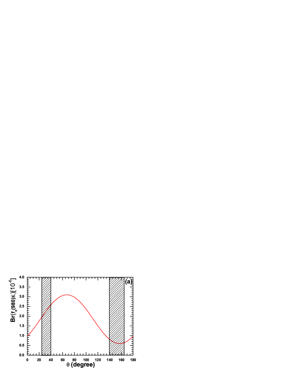
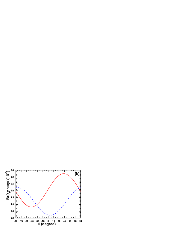
Figure 2: The dependence of the branching ratios for $\bar{B}^{0}_{s}\to f_{0}(980)K^{0}$ (a) and $\bar{B}^{0}_{s}\to f_{0}(1500)K^{0}$ (b) on the mixing angle $\theta$ using the inputs derived from QCD sum rules. For the right panel, the dashed (solid) curve is plotted in scenario I (II). The vertical bands show two possible ranges of $\theta$: $25^{\circ}<\theta<40^{\circ}$ and $140^{\circ}<\theta<165^{\circ}$.

Table 2: Decay amplitudes for $\bar{B}^{0}_{s}\to f_{0}(980)K^{0},f_{0}(1500)K^{0}$ ($\times 10^{-2}\mbox{GeV}^{3}$).

$\bar{s}s$		$F^{K}_{e}$	$M^{K}_{e}$	$M^{K}_{a}$	$F^{K}_{a}$	$M^{f_{0}}_{e}$
$f_{0}(980)K^{0}$ (SI)		-1.0	$0.2+0.5i$	$-0.4-0.1i$	$2.2-10.3i$	$-5.7-5.1i$
$f_{0}(1500)K^{0}$ (SI)		1.8	$-0.6+0.8i$	$-0.1-0.2i$	$6.6+13.4i$	$-2.2-8.1i$
$f_{0}(1500)K^{0}$ (SII)		-2.4	$0.6+0.07i$	$-0.5-0.04i$	$-0.8-21.1i$	$-6.3-1.7i$
$\bar{n}n$		$F^{f_{0}}_{e}$	$M^{f_{0},T}_{e}$	$M^{f_{0}}_{e}$	$M^{f_{0}}_{a}$	$F^{f_{0}}_{a}$
$f_{0}(980)(\bar{n}n)K^{0}$ (SI)		7.2	$57.5+47.6i$	$-10.1-9.5i$	$0.4+0.4i$	$1.9-8.7i$
$f_{0}(1500)(\bar{n}n)K^{0}$ (SI)		-7.6	$20.9+77.1i$	$-2.6-15.1i$	$-0.7+0.7i$	$6.8+11.8i$
$f_{0}(1500)(\bar{n}n)K^{0}$ (SII)		14.6	$57.9+14.3i$	$-10.7-2.9i$	$0.9+0.1i$	$-1.4-17.8i$

In table II, we list values of the factorizable and non-factorizable amplitudes from the emission and annihilation topology diagrams of the decays $\bar{B}^{0}_{s}\to f_{0}(980)K,f_{0}(1500)K$. $F^{K}_{e(a)}$ and $M^{K}_{e(a)}$ are the $K$ emission (annihilation) factorizable contributions and non-factorizable contributions from penguin operators respectively. Similarly, $F^{f_{0}}_{e(a)}$ and $M^{f_{0}}_{e(a)}$ denote as the contributions from $f_{0}$ emission (annihilation) factorizable contributions and non-factorizable contributions from penguin operators respectively. It is easy to see that $F^{f_{0}}_{e(a)}$ and $M^{f_{0}}_{e(a)}$ are larger than $F^{K}_{e(a)}$ and $M^{K}_{e(a)}$, that is $f_{0}$- emission diagrams give large contributions. $M^{f_{0},T}_{e}$ denotes the $f_{0}$ emission non-factorizable contribution from tree operator $O_{2}$. From the table, one can find that the contributions from $n\bar{n}$ component of $f_{0}$ are larger than those from $s\bar{s}$ component, the one reason is that $M^{f_{0},T}_{e}$ from the operator $O_{2}$ is much larger than other amplitudes. Furthermore, ${\cal B}(\bar{B}^{0}_{s}\to f_{0}(n\bar{n})K)$ is about two or five times of ${\cal B}(\bar{B}^{0}_{s}\to f_{0}(s\bar{s})K)$. Certainly, as to the decay $\bar{B}^{0}_{s}\to f_{0}(1500)K$ in SI, the difference is greater. One can see the values of ${\cal B}(\bar{B}_{s}\to f_{0}(1500)(n\bar{n})K)$ in SI and SII are close to each other, but the values of ${\cal B}(\bar{B}^{0}_{s}\to f_{0}(1500)(s\bar{s})K)$ in the two scenarios are much differ, which results the total branching ratios have an apparent difference between these two scenarios (shown in figur 2(b)).

In figure 2, we plot the branching ratios as functions of the mixing angle $\theta$. If the mixing angle $\theta$ falls into the range of $25^{\circ}<\theta<40^{\circ}$, the branching ratio of $\bar{B}^{0}_{s}\to f_{0}(980)K$ is:

$$2.0\times 10^{-6}<{\cal B}(\bar{B}^{0}_{s}\to f_{0}(980)K)<2.6\times 10^{-6},$$ (41)

while $\theta$ lies in the range of $140^{\circ}<\theta<165^{\circ}$, ${\cal B}(\bar{B}^{0}_{s}\to f_{0}(980)K)$ is roughly $6.5\times 10^{-7}$. The dependence of the branch ratio of $\bar{B}^{0}_{s}\to f_{0}(980)K$ is strong in the whole mixing angle range, but not sensitive in some ranges, for example, $140^{\circ}<\theta<165^{\circ}$. As to the decay $\bar{B}^{0}_{s}\to f_{0}(1500)K$, because there are more discrepancies for the structure of $f_{0}(1500)$, we do not show the possible allowed mixing angle range in Fig.2(b). Lattice QCD predicted that the mass of the ground state scalar glueball is around $1.5-1.8$ GeV glueball ; cheny , so the three mesons $f_{0}(1370),f_{0}(1500)$ and $f_{0}(1710)$ become the potential candidates. The mixing matrix can be written as wwang2

$$\left(\begin{array}[]{c}f_{0}(1710)\\ f_{0}(1500)\\ f_{0}(1370)\end{array}\right)=\left(\begin{array}[]{ccc}a_{1}&a_{2}&a_{3}\\ b_{1}&b_{2}&b_{3}\\ c_{1}&c_{2}&c_{3}\end{array}\right)\left(\begin{array}[]{c}G\\ \bar{s}s\\ \bar{n}n\end{array}\right).$$ (51)

For each physical scalar meson, the corresponding component coefficients satisfy the normalization condition, so we have $\sqrt{|b_{1}|^{2}+|b_{2}|^{2}+|b_{3}|^{2}}=1$ for the meson $f_{0}(1500)$. For the earlier lattice calculations predicting the scalar glueball mass to be about $1550$ MeV and the decay width of $f_{(}1500)$ being not compatible with a simple $q\bar{q}$ state amsler0 , Amsler and Close claimed that $f_{0}(1500)$ is primarily a scalar glueball amsler . But in the $SU(3)$ symmetry limit, Cheng et al. reanlyze all existing experimental data and find that $f_{0}(1500)$ is a pure SU(3) octet with a very tiny glueball content. Their results for the mixing coefficients are given in the following mixingch

$$\left(\begin{array}[]{c}f_{0}(1710)\\ f_{0}(1500)\\ f_{0}(1370)\end{array}\right)=\left(\begin{array}[]{ccc}0.93&0.17&0.32\\ -0.03&0.84&-0.54\\ -0.36&0.52&0.78\end{array}\right)\left(\begin{array}[]{c}G\\ \bar{s}s\\ \bar{n}n\end{array}\right).$$ (61)

From above Equation, it is ease to see that $f_{0}(1710)$ is composed primarily of a scalar glueball. This conclusion is also supported by an improved LQCD calculation cheny , which predicts that the mass of the scalar glueball is $1710\pm 50\pm 80$ MeV. Here we use the mixing coefficients for $f_{0}(1500)$ given in Eq.(61) and neglect the tiny component of glueball, that is $\mid f_{0}(1500)\rangle=0.84\mid s\bar{s}\rangle-0.54\mid n\bar{n}\rangle$. The branching ratios in two scenarios given as:

$${\cal B}(\bar{B}^{0}_{s}\to f_{0}(1500)K^{0}) = 9.7\times 10^{-7},\mbox{ Scenario I},$$

$${\cal B}(\bar{B}^{0}_{s}\to f_{0}(1500)K^{0}) = 9.5\times 10^{-7},\mbox{ Scenario II},$$ (62)

which is obtained by the mixing angle taken as $-32.7^{\circ}$. From these results, it is difficult to determine which scenario is more preferable than the other.

Now we turn to the evaluations of the CP-violating asymmetries of the considered decays in PQCD approach. For the neutral decays $\bar{B}^{0}_{s}\to f_{0}(980)K_{S},f_{0}(1500)K_{S}$, there are both direct $CP$ asymmetry $A^{dir}_{CP}$ and mixing-induced $CP$ asymmetry $A^{mix}_{CP}$. The time dependent $CP$ asymmetry of $B^{0}_{s}$ decay into a $CP$ eigenstate $f$ is defined as

$${\cal A}_{CP}(t)={\cal A}^{dir}_{CP}(B^{0}_{s}\to f)\cos(\Delta m_{s})+{\cal A}^{mix}_{CP}(B^{0}_{s}\to f)\sin(\Delta m_{s}),$$ (63)

with

$${\cal A}^{dir}_{CP}(B^{0}_{s}\to f) = \frac{|\lambda|^{2}-1}{1+|\lambda|^{2}},\;\;\;{\cal A}^{mix}_{CP}(B^{0}_{s}\to f)=\frac{2Im\lambda}{1+|\lambda|^{2}},$$ (64)

$$\lambda = \eta e^{-2i\beta}\frac{{\cal A}(\bar{B}^{0}_{s}\to f)}{{\cal A}(B^{0}_{s}\to f),}$$ (65)

where $\eta=\pm 1$ depends on the $CP$ eigenvalue of $f$, $\Delta m_{s}$ is the mass difference of the two neutral $B_{s}$ meson eigenstates. Here we only give the direct CP asymmetries.

Table 3: Direct $CP$ asymmetries (in units of %) of $\bar{B}^{0}_{s}\to f_{0}(980)K^{0},f_{0}(1500)K^{0}$ decays for $n\bar{n}$ and $s\bar{s}$ components, respectively.

Channel	Scenario I	Scenario II
$\bar{B}^{0}_{s}\to f_{0}(980)(n\bar{n})K^{0}$	$-57.0$	-
$\bar{B}^{0}_{s}\to f_{0}(980)(s\bar{s})K^{0}$	$0$	-
$\bar{B}^{0}_{s}\to f_{0}(1500)(n\bar{n})K^{0}$	$17.6$	$-94.8$
$\bar{B}^{0}_{s}\to f_{0}(1500)(s\bar{s})K^{0}$	$0$	$0$

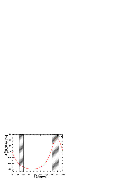
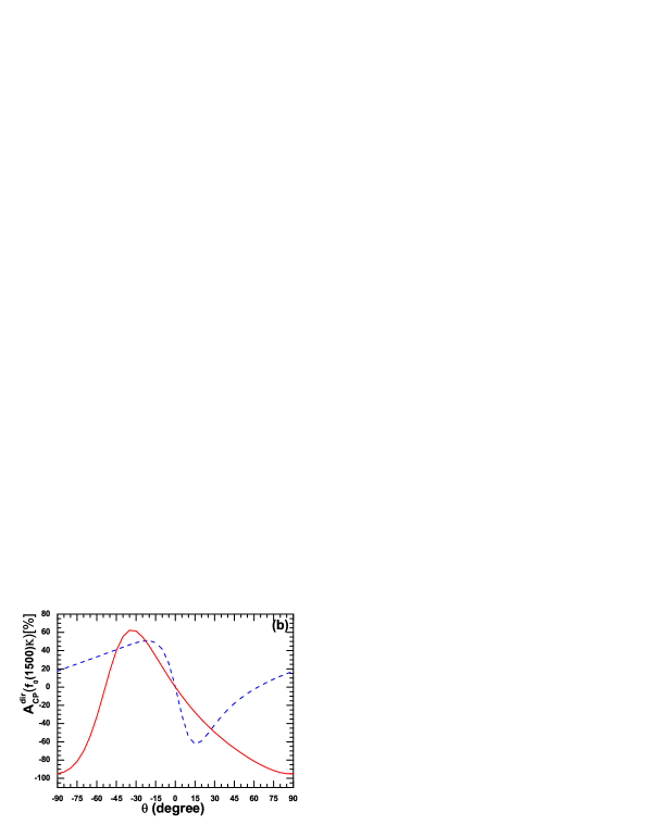
Figure 3: The dependence of the direct CP asymmetries for $\bar{B}^{0}_{s}\to f_{0}(980)K$ (a) and $\bar{B}^{0}_{s}\to f_{0}(1500)K$ (b) on the mixing angle $\theta$. For the right panel, the dashed (solid) curve is plotted in scenario I (II). The vertical bands show two possible ranges of $\theta$: $25^{\circ}<\theta<40^{\circ}$ and $140^{\circ}<\theta<165^{\circ}$.

In $\bar{B}^{0}_{s}\to f_{0}(s\bar{s})K$, there is no tree contribution at the leading order, so the direct CP asymmetry is naturally zero. As $\bar{B}^{0}_{s}\to f_{0}(n\bar{n})K$, the corresponding direct CP asymmetries are listed in table III. For the decay $\bar{B}^{0}_{s}\to f_{0}(1500)K$, the amplitudes from the non-factorizable $f_{0}$-emission and annihilation topologies, that is $M_{e}^{f_{0}}$ and $F_{a}^{f_{0}}$, are constructive in scenario II but are destructive in scenario I (seen in table II). Furthermore, the contributions from the factorizable $f_{0}$-emission diagrams have an opposite sign between scenario I and II (which is because that the decay constant of $f_{0}(1500)$ is opposite in two scenarios). These reasons result that there exists a great difference for the direct CP asymmetries of $\bar{B}^{0}_{s}\to f_{0}(1500)(n\bar{n})K$ in two scenarios (shown in table III). The dependence of the direct CP violating asymmetries for these decays are shown in Fig.3. From Fig.3(a), we can see that the signs of the direct CP asymmetries in the two allowed mixing angle ranges are opposite, it gives the hint that one can determine the mixing angle by comparing with the future experimental results. For the decay $\bar{B}^{0}_{s}\to f_{0}(1500)K$, if we still use the mixing scheme given by Eq.(61) for $f_{0}(1500)$, the direct CP asymmetry is

$${\cal A}^{dir}_{CP}(\bar{B}^{0}_{s}\to f_{0}(1500)K^{0}) = 47.4\%,\qquad\mbox{ scenario I},$$

$${\cal A}^{dir}_{CP}(\bar{B}^{0}_{s}\to f_{0}(1500)K^{0}) = 62.8\%,\qquad\mbox{ scenario II}.$$ (66)

Although the CP asymmetry for the decay $\bar{B}^{0}_{s}\to f_{0}(1500)K^{0}$ is large, it is difficult to measure it, since its branching ratio is small.

V Conclusion

In this paper, we calculate the branching ratios and the direct CP-violating asymmetries of $\bar{B}^{0}_{s}\to f_{0}(980)K,f_{0}(1500)K$ decays in the PQCD factorization approach. From our calculations and phenomenological analysis, we find the following results:

• In general, the contributions from $f_{0}$-emission diagrams are larger than those from $K$-emission diagrams. Especially, the $f_{0}$-emission non-factorizable contribution from tree operator $O_{2}$ is quite larger than other amplitudes. For the decays $\bar{B}^{0}_{s}\to f_{0}(980)K,f_{0}(1500)K$, the contributions from $n\bar{n}$ component are larger than those from $s\bar{s}$ component in two scenarios.

• Using the wave functions and the values of relevant input parameters, we find the numerical results of the corresponding form factors $\bar{B}^{0}_{s}\to f_{0}(s\bar{s})$ at zero meomentum transfer

  $$F^{\bar{B}^{0}_{s}\to f_{0}(980)}_{0}(q^{2}=0) = 0.33^{+0.02+0.02+0.02}_{-0.01-0.01-0.01},\quad\mbox{ scenario I},$$ (67)

  $$F^{\bar{B}^{0}_{s}\to f_{0}(1500)}_{0}(q^{2}=0) = -0.25^{+0.01+0.06+0.04}_{-0.00-0.05-0.03},\quad\mbox{ scenario I},$$ (68)

  $$F^{\bar{B}^{0}_{s}\to f_{0}(1500)}_{0}(q^{2}=0) = 0.59^{+0.06+0.04+0.05}_{-0.06-0.03-0.05},\quad\;\;\;\mbox{ scenario II}.$$ (69)

  The values of $F^{\bar{B}^{0}_{s}\to f_{0}(1500)}_{0}(q^{2}=0)$ for two scenarios can be used to identify which scenario is favored by compare with the future experimental results.

• If the mixing angle $\theta$ falls into the range of $25^{\circ}<\theta<40^{\circ}$, the branching ratio of $\bar{B}^{0}_{s}\to f_{0}(980)K$ is

  $$2.0\times 10^{-6}<{\cal B}(\bar{B}^{0}_{s}\to f_{0}(980)K)<2.6\times 10^{-6},$$ (70)

  while $\theta$ lies in the range of $140^{\circ}<\theta<165^{\circ}$, ${\cal B}(\bar{B}^{0}_{s}\to f_{0}(980)K)$ is about $6.5\times 10^{-7}$.

• if we identify the meson $f_{0}(1500)$ as a pure SU(3) octet state and use the mixing scheme giving by $\mid f_{0}(1500)\rangle=0.84\mid s\bar{s}\rangle-0.54\mid n\bar{n}\rangle$, one can find that the branching ratios in two scenarios are both close to $1.0\times 10^{-6}$. Although the CP asymmetry for the decay $\bar{B}^{0}_{s}\to f_{0}(1500)K^{0}$ is large, it is difficult to measure it, since its branching ratio is small.

References

• (1) A. K. Giri , B. Mawlong, R. Mohanta Phys. Rev. DΒ 74, 114001 (2006).
• (2) H. Y. Cheng, K. C. Yang Phys. Rev. DΒ 71, 054020 (2005).
• (3) H. Y. Cheng, C.K. Chua, K. C. Yang, Phys. Rev. DΒ 73, 014017 (2006).
• (4) H. Y. Cheng, C.K. Chua, K. C. Yang, Phys. Rev. DΒ 77, 014034 (2008).
• (5) C. H. Chen, Phys. Rev. DΒ 67, 014012 (2003).
• (6) C. H. Chen, Phys. Rev. DΒ 67, 094011 (2003).
• (7) W. Wang, Y. L. Shen, Y. Li, C. D. LΓΌ Phys. Rev. DΒ 74, 114010 (2006).
• (8) Z.Q. Zhang and Z.J. Xiao, Chin.Phys.C 33(07):508-515 (2009).
• (9) Z.Q. Zhang and Z.J. Xiao, Chin.Phys.C 34(05):528-534 (2010).
• (10) Y. L. Shen, W. Wang, J. Zhu and C. D. LΓΌ, Eur.Phys.J.C 50:877-887 (2007).
• (11) J. Botts and G. Sterman, Nucl. Phys. B 225, 62 (1989).
• (12) H.N. Li and G.Sterman, Nucl. Phys. B 381, 129 (1992).
• (13) N.Brambilla et al., (Quarkonium Working Group), CERN-2005-005, hep-ph/0412158; M.P. Altarelli and F.Teubert, Int. J. Mod.Phys. A 23, 5117 (2008).
• (14) M. Artuso et al., ”B, D and K decays”, Report of Working Group 2 of the CERN workshop on Flavor in the Era of the LHC, Eur. Phys. J. C 57:309-492 (2008).
• (15) N.A.Β Tornqvist, Phys. Rev. Lett. 49, 624 (1982).
• (16) G.L.Β Jaffe, Phys. Rev. DΒ 15, 267 (1977); Erratum-ibid.Phys. Rev. DΒ 15 281 (1977); A.L.Β Kataev, Phys. Atom. Nucl. 68, 567 (2005), Yad. Fiz. 68, 597 (2005); A.Β Vijande, A. Valcarce, F.Β Fernandez and B.Β Silvestre-Brac, Phys. Rev. D 72, 034025 (2005).
• (17) H.Y. Cheng, Phys. Rev. DΒ 67, 034024 (2004).
• (18) A.G.Grozin and M.Neubert, Phys. Rev. DΒ 55, 272 (1977); M.Beneke and T.Feldmann, Nucl. Phys.B 592,3 (2001).
• (19) H.Kawamura, J.Kodaira, C.F. Qiao and K. Tanaka, Phys. Lett. B 523, 111 (2001); Mod.Phys.Lett.A 18,799 (2003).
• (20) C.D. LΓΌ, M.Z. Yang, Eur.Phys.J.C 28, 515 (2003).
• (21) H.N. Li, Phys. Rev. DΒ 66, 094010 (2002).
• (22) H.N. Li and B. Tseng, Phys. Rev. DΒ 57, 443 (1998).
• (23) G. Buchalla, A.J. Buras, M.E. Lautenbacher, Rev. Mod. Phys. 68, 1125 (1996).
• (24) A. Ali, G. Kramer, C.D. LΓΌ, Phys. Rev. DΒ 58, 094009 (1998).
• (25) Z.J. Xiao, Z.Q. Zhang, X. Liu, L.B. Guo, Phys. Rev. DΒ 78, 114001 (2008).
• (26) Particle Data Group, C.Β Amsler et al., Phys. Lett. BΒ 667, 1 (2008).
• (27) V.M. Braun, G.P. Korchemsky, D. Mueller, Prog. Part. Nucl. Phys. 51:311-398, (2003).
• (28) A. Ali et al., Phys. Rev. D 76, 074018 (2007), Z.J. Xiao, X.F. Chen and D.Q. Guo, Eur. Phys. J. C 50:363-371 (2007).
• (29) R.H. Li et al., Phys. Rev. DΒ 79, 014013 (2009).
• (30) G. S. Bali, et al. [UKQCD Collaboration], Phys. Lett. B 309, 378 (1993); H. Chen, J. Sexton, A. Vaccarino and D. Weingarten, Nucl. Phys. Proc. Suppl. 34, 357 (1994); C. J. Morningstar and M. J. Peardon, Phys. Rev. D 60, 034509 (1999) ; A. Vaccarino and D. Weingarten, Phys. Rev. D 60, 114501 (1999).
• (31) Y. Chen et al., Phys. Rev. DΒ 73, 104516 (2006).
• (32) W. Wang, Y.L. Shen and C.D. LΓΌ, arXiv:hep-ph/0909.4141v1.
• (33) C. Amsler et al., Phys. Lett. BΒ 342, 433 (1995); Phys. Lett. BΒ 340, 259 (1994).
• (34) C. Amsler and F.E. Close, Phys.Lett.B 353,385 (1995).
• (35) H. Y. Cheng, C. K. Chua and K. F. Liu, Phys. Rev. D 74, 094005 (2006).