Active and hibernating turbulence in minimal channel flow of Newtonian and polymeric fluids

Abstract

Turbulent channel flow of drag-reducing polymer solutions is simulated in minimal flow geometries. Even in the Newtonian limit, we find intervals of “hibernating” turbulence that display many features of the universal maximum drag reduction (MDR) asymptote observed in polymer solutions: weak streamwise vortices, nearly nonexistent streamwise variations and a mean velocity gradient that quantitatively matches experiments. As viscoelasticity increases, the frequency of these intervals also increases, while the intervals themselves are unchanged, leading to flows that increasingly resemble MDR.

The energy dissipated in turbulent channel or pipe flow of a liquid can be dramatically reduced by low levels of long-chain polymer additives (Virk, 1975; Graham, 2004; White and Mungal, 2008). The most striking qualitative feature of this phenomenon is the existence of a so-called maximum drag reduction (MDR) asymptote (Virk, 1975). For a given flow geometry at a given pressure drop (i.e. at a given Reynolds number Re), there is an asymptotic maximum flow rate that can be achieved through addition of polymers. Changing the concentration, molecular weight or even the chemical structure of the additives has no effect on this asymptotic value. This universality is the major puzzle of drag reduction.

Turbulent flow in or near the MDR regime displays important differences from Newtonian turbulence. Its most commonly discussed signature is a distinctive mean velocity profile $U_{\mathrm{mean}}(y)$ that displays clear log-law behavior well-approximated by a formula given by Virk: $U_{\mathrm{mean}}^{+}=11.7\>\ln y^{+}-17.0$ (Virk, 1975) (Superscript “+” denotes quantities nondimensionalized in inner velocity and length scales $\sqrt{\tau_{\mathrm{w}}/\rho}$ and $\eta/\sqrt{\rho\tau_{w}}$; $\tau_{\mathrm{w}}$ is the time- and area averaged wall shear stress, $\eta$ and $\rho$ are fluid viscosity and density and $y$ is distance from the wall.) Additionally, streamwise vortices, which dominate near-wall dynamics in Newtonian turbulence, are significantly weakened at MDR. Low-speed streaks become much less wavy in the streamwise direction and the streak spacing is substantially larger (White et al., 2004; Housiadas et al., 2005; Li et al., 2006; Xi and Graham, 2010). In addition, the Reynolds shear stress near MDR is substantially smaller than in Newtonian turbulence (Ptasinski et al., 2001; Warholic et al., 1999, 2001; Ptasinski et al., 2003). Indeed, the smallness of Reynolds shear stress is a central issue in a recent phenomenological model of MDR Procaccia et al. (2008).

Based on these observations, many researchers have suggested that turbulence in the MDR regime is “transitional” White and Mungal (2008) or “marginal” Procaccia et al. (2008) in some sense that is not yet well-defined, and that the spatiotemporal flow structures that sustain turbulence in this regime are substantially different from those of normal Newtonian turbulence. In the latter case, one simulation approach that has been fruitful in identifying the self-sustaining structures is the so-called minimal flow unit (MFU) approach Jiménez and Moin (1991); Webber et al. (1997). This approach identifies the smallest flow domain (at a given Reynolds number) in which turbulence can be sustained. Accordingly, temporally intermittent phenomena can be identified more readily than in a large box, where spatial averages incorporate different regions in which the instantaneous behavior may be very different. The present work is the first to address the relevance of this approach for understanding MDR.

We focus on plane Poiseuille flow with fixed pressure drop. Streamwise, wall-normal and spanwise directions are denoted $x$, $y$, and $z$, respectively. The no-slip boundary condition applies at $y=\pm 1$ and periodic boundary conditions apply in $x$ and $z$; the periods in these directions are $L_{x}$ and $L_{z}$. Lengths are scaled with half-channel height $l$ and velocities with the Newtonian laminar centerline velocity $U$ at the given pressure drop. Time $t$ is scaled with $l/U$ and pressure $p$ with $\rho U^{2}$. The governing equations are:

$$\frac{D\boldsymbol{v}}{Dt}=-\boldsymbol{\nabla}p+\frac{\beta}{\textit{Re}}\nabla^{2}\boldsymbol{v}+\frac{2\left(1-\beta\right)}{\textit{Re}\textit{Wi}}\left(\boldsymbol{\nabla}\cdot\boldsymbol{\tau}_{\mathrm{p}}\right),\boldsymbol{\nabla}\cdot\boldsymbol{v}=0$$ (1)

$$\begin{split}\frac{\textit{Wi}}{2}\left(\frac{D\boldsymbol{\alpha}}{Dt}-\boldsymbol{\alpha}\cdot\boldsymbol{\nabla v}-\left(\boldsymbol{\alpha}\cdot\boldsymbol{\nabla v}\right)^{\mathrm{T}}\right)=-\frac{b}{b+5}\boldsymbol{\tau}_{\mathrm{p}},\end{split}$$ (2)

$$\boldsymbol{\tau}_{\mathrm{p}}=\frac{b+5}{b}\left(\frac{\boldsymbol{\alpha}}{1-\frac{\mathrm{tr}(\boldsymbol{\alpha})}{b}}-\left(1-\frac{2}{b+2}\right)\boldsymbol{\delta}\right).$$ (3)

Eq. (1) describes conservation of momentum and mass, and the polymer conformation and stress tensors $\boldsymbol{\alpha}$ and $\boldsymbol{\tau}_{\mathrm{p}}$ are described by the FENE-P constitutive equation for a bead-spring dumbbell model of a polymer in solution ((Eqs. 2) and (3)) (Bird et al., 1987). Reynolds number $\textit{Re}\equiv\rho Ul/\eta$, Weissenberg number $\textit{Wi}\equiv 2\lambda U/l$ ($\lambda$ is the polymer relaxation time), viscosity ratio $\beta\equiv\eta_{\mathrm{s}}/\eta$ ($\eta_{s}$ is the solvent contribution to zero-shear viscosity), and $b$ is the upper limit of the extension of polymer. All simulations reported here are at $\textit{Re}=3600,\beta=0.97,b=5000$. The numerical integration procedure is described in (Xi and Graham, 2010).

A rigorous search for MFUs would consider the parameter dependence of both $L_{x}^{+}$ and $L_{z}^{+}$, a task involving an impractically large number of simulation runs. Here we fix $L_{x}^{+}=360$ (which is in the range of streamwise sizes of Newtonian MFU Jiménez and Moin (1991); Webber et al. (1997)) and vary $L_{z}^{+}$ only. Although both length scales depend on parameters, $L_{z}^{+}$ is arguably the quantity of more interest: the dominant structures are the streamwise streaks and the streamwise vortices aligned alongside them; $L_{z}^{+}$ restricts the streak spacing and the size of the vortices.

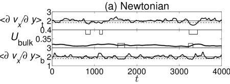
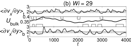
Figure 1: Mean shear rates at the walls (“b”–bottom, “t”–top) and bulk velocity $U_{\textrm{bulk}}$ as functions of time for typical segments of (a) Newtonian and (b) viscoelastic ($\textit{Wi}=29$) simulations. Solid and dashed lines show $\langle\partial v_{x}/\partial y\rangle=2$ and $\langle\partial v_{x}/\partial y\rangle=1.8$, respectively. In laminar flow, $U_{\textrm{bulk}}=2/3$.

Fig. 1 shows time series of instantaneous bulk average velocity $U_{\textrm{bulk}}$ and area-averaged shear rate $\langle\partial v_{x}/\partial y\rangle$ at the top and bottom walls for (a) Newtonian flow and (b) viscoelastic flow at $\textit{Wi}=29$, where $DR\%=26$ and $L_{z}^{+}$ has increased from $140$ to $250$. In the Newtonian case, Fig. 1(a), one occasionally observes long-lasting periods when the shear rate at one or both walls is substantially lower than the average value of 2 – for example the time interval $3200<t<3400$. By momentum conservation, the bulk velocity increases during these periods. A similar observation was made in the Newtonian MFU study of Webber et al. Webber et al. (1997). These periods will be termed “hibernation”, in contrast to the “active” turbulence found outside them. As Wi increases, hibernation periods become increasingly frequent (Fig. 1(b)) – since the bulk velocity increases during these periods, they contribute substantially to drag reduction.

To systematically identify hibernation events, two criteria are used: (1) area-averaged wall shear rate at one or both walls drops below a cutoff value $\langle\partial v_{x}/\partial y\rangle|_{\mathrm{cutoff}}=1.8$; and (2) it stays there for longer than a certain amount of time $\Delta t_{\mathrm{cutoff}}=50$. Hibernating periods so identified are shown in the middle panels of Fig. 1 as rectangular signals, on the top or bottom of the plot according to the wall(s) on which the criterion is satisfied.

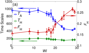
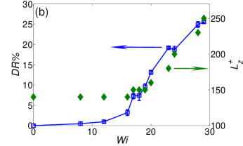
Figure 2: (a) Time scales and fraction of time spent in hibernation and (b) level of drag reduction and spanwise box size, as functions of Wi. (At the relatively low Reynolds number considered here, the flow laminarizes for $\textit{Wi}\gtrsim 31$).

Based on this identification scheme, Fig. 2(a) shows, as functions of Wi, the mean duration of the hibernation periods $T_{H}$, mean duration of active periods $T_{A}$, and fraction of time spent in hibernation $F_{H}$. Corresponding results for minimal spanwise box size and level of drag reduction are in Fig. 2(b). Notice that the average duration $T_{H}$ of a hibernating period is almost completely insensitive to Wi. In contrast, the average duration $T_{A}$ of an active turbulence phase decreases substantially after onset of drag reduction. Therefore, at high Wi, viscoelasticity compresses the lifetime of active turbulence intervals, while having virtually no effect on hibernation.

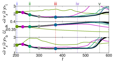
Figure 3: A hibernation event. Thick black lines are results at $\textit{Wi}=29$ ($200\leqslant t\leqslant 600$ in Fig. 1(b)). Colored lines are from Newtonian simulations started at the dots, using velocity fields from the $\textit{Wi}=29$ simulation.

The insensitivity of $T_{H}$ to Wi suggests that flow during hibernation does not strongly stretch polymer molecules. Indeed, at $\textit{Wi}=29$ the peak value of $\langle\alpha_{yy}\rangle$, which is closely associated with streamwise vortex suppression (Procaccia et al., 2008; Stone et al., 2004; Li and Graham, 2007), drops from about 210 in active turbulence to about 5 during hibernation, a 40-fold reduction. These results suggest that hibernation should be very similar in the Newtonian and viscoelastic cases. To test this possibility, velocity fields from time instants before and during a hibernation event at $\textit{Wi}=29$ were used as initial conditions for a Newtonian simulation, the trajectories of which were then compared with those from the original viscoelastic simulation. Fig. 3 illustrates the original viscoelastic trajectory (thick black line) as well as Newtonian trajectories (colors) started at various times. For the Newtonian run starting before any sign of hibernation is observed ($t=205$), active turbulence is sustained. However, runs started from later times show that once the system begins to enter hibernation, removing the polymer stress does not cause turbulence to revert to an active state, although the depth and duration of hibernation are weakly dependent on the start time.

(a)                                                                           

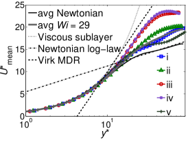
(b)                                                                           

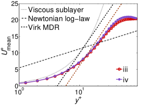
(c)                                                                           

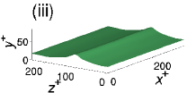
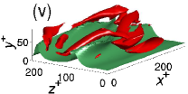
Figure 4: (a): Instantaneous mean velocity profiles of snapshots i-v (colors), and time-averaged profiles in the Newtonian and $\textit{Wi}=29$ cases. (The latter are plotted in terms of conventional wall units.) (b): Instantaneous mean velocity profiles from time instants iii and iv plotted in conventional wall units. For comparison, a downward-shifted plot of the Virk log-law is also shown. (c): flow structures of typical snapshots in hibernation (iii) and active turbulence (v). Green sheets are isosurfaces $v_{x}=0.3$; pleats correspond to low-speed streaks; red tubes are isosurfaces of streamwise-vortex intensity $Q_{\mathrm{2D}}=0.02$, calculated by applying the $Q$-criterion of vortex indentification Jeong and Hussain (1995) in the $yz$ plane Li and Graham (2007); Xi and Graham (2010).

To better understand these results, we examine more closely the hibernating period shown in Fig. 3. Several time instants are selected as marked: (i) is just before turbulence enters hibernation; (ii) is on the path toward hibernation; (iii) and (iv) are within hibernation; (v) is after turbulence becomes reactivated. Fig. 4a shows instantaneous area-averaged velocity profiles in the bottom half of the channel at these instants, plotted in inner units based on the instantaneous wall shear stress at the bottom wall (denoted by the superscript ^∗ rather than ⁺). By collapsing the viscous sublayer behavior onto a single curve, this choice of scaling best exposes the nature of and differences between the various time instants shown. In active turbulence (i and v), the profiles fluctuate substantially. Profiles for snapshots completely in hibernation (iii and iv) are fundamentally different. In particular, in the range $15\lesssim y^{*}\lesssim 40$, both profiles show a clear log-law relationship with a slope very close to (within $10\%$ of) the Virk MDR asymptotic slope of 11.7 Virk (1975). (The differences between the intercepts is smaller than the scatter of the available data.) The figure also shows the time-averaged mean velocity profiles for the Newtonian flow (which has a log-law region in good agreement with the classical result $U_{\mathrm{mean}}^{+}=2.5\ln y^{+}+5.5$) and the flow at $\textit{Wi}=29$, which is, as expected, intermediate between the Newtonian and MDR profiles. To illustrate that the choice of scaling does not affect the conclusion that velocity profiles in hibernation display a log-law slope close to the Virk results, Fig. 4b shows the curves from time instants iii and iv in conventional wall units. Although shifted downward from the Virk profile (because in the instantaneous wall shear stress is less than the time-averaged wall shear stress), the log-law slope remains within $20\%$ of the Virk value. The Newtonian hibernation periods (not shown, for brevity) are very similar and the Virk slope is observed there as well.

Fig. 4c shows flow structures corresponding to time instants iii and v. Within active periods (v), turbulence shows the expected highly 3D structure of streamwise vortices and low-speed streaks Robinson (1991); Jiménez and Moin (1991); Waleffe (1997). During hibernation (iii), streamwise vortices are significantly weaker; low-speed streaks are still observed, but are weak and only weakly dependent on $x$. (The low shear events observed in the Newtonian MFU study of Webber et al. Webber et al. (1997) also display weak streamwise dependence.) Weak streamwise vorticity and three-dimensionality are distinct characteristics of the MDR regime (Virk, 1975; White et al., 2004; Housiadas et al., 2005; Li et al., 2006; White and Mungal, 2008). The weak effect of viscoelasticity on hibernating turbulence may lie in its nearly streamwise-invariant kinematics. In the limiting case of a streamwise invariant steady flow, material lines cannot stretch exponentially Ottino (1989); accordingly, polymer stretch in such a flow will not be substantial. Finally, the Reynolds shear stress during hibernation drops to very low values relative to active turbulence, where it peaks at about 0.8; the peak value during hibernation is about $0.3$. Again, this result is consistent with observations in the MDR regime Ptasinski et al. (2001, 2003); Warholic et al. (1999, 2001).

The qualitative picture that emerges from these simulations is thus the following. Active turbulence generates substantial stretching of polymer molecules. The resulting stresses act to suppress this turbulence and drive the flow toward a very weakly turbulent hibernating regime. During hibernation the polymer molecules are no longer strongly stretched and relax toward equilibrium. Eventually, hibernation ends as new turbulent fluctuations begin to grow, and the system transits back into active turbulence. The active turbulence again stretches polymer chains and the (stochastic) cycle repeats.

In this picture, experimental observations in which the Virk MDR mean velocity profile is found correspond to a limiting situation – not achieved at the low Reynolds number and small boxes studied here – where the fraction of time and space occupied by active turbulence becomes small enough that the hibernating regime dominates the statistics. Active turbulence cannot vanish entirely, because it is known that on average, the polymer molecules carry a substantial fraction of the mean shear stress (Warholic et al., 1999; Ptasinski et al., 2003), and since hibernating turbulence does not stretch polymers, some active turbulence must remain. These considerations lead to a new picture of turbulence in the MDR regime as a state in which hibernating turbulence is the norm, with active turbulence arising intermittently in space and time only to be suppressed by the polymer stretching that it induces.

This study focused on MFU flows at low Reynolds number, allowing analysis of an extensive data set in a regime where flow structures are relatively simple. Remarkably, even this regime displays clear signatures of the features of MDR commonly associated with higher Reynolds numbers. (Though it should be noted that the MDR asymptote is experimentally observed at values of Re all the way down into the laminar-turbulent transition regime Virk (1975).) To carefully evaluate the generality of picture just presented, future work will require simulations at higher Re and large boxes in combination with pattern analysis tools that can identify spatiotemporally localized regions of active and hibernating turbulence.

In addition, attention must be focused on the hibernation phenomenon. Waleffe has identified a class of nonlinear traveling wave solutions in the plane Couette and Poiseuille geometries – saddle points in phase space – that share many characteristics with hibernating turbulence, specifically weak streamwise vortices and weak streamwise dependence Wang et al. (2007). At least one family of these solutions has vanishing streamwise dependence and Reynolds shear stress as $\textit{Re}\rightarrow\infty$. Similarly, other researchers Schneider et al. (2007, 2008); Duguet et al. (2008) have identified both simple and chaotic saddle trajectories, “edge states”, that lie on the boundary between laminar and turbulent dynamics. These observations may allow us to make rigorous the qualitative notion described in the introduction that the MDR regime is transitional or marginal – it may be that hibernating turbulence is very near in phase space to the boundary between laminar and turbulent flow. Finally, a better understanding of hibernation may lead to strategies for active flow control to maintain turbulence in a state of hibernation and thus dramatically reduce skin friction.

The authors thank Fabian Waleffe for many helpful discussions. The code used here is based on ChannelFlow by John F. Gibson, whose assistance we gratefully acknowledge. This work is supported by the National Science Foundation (DDDAS-SMRP-0540147, CBET-0730006).

References

- Virk (1975) P. S. Virk, AIChE J. 21, 325 (1975).
- Graham (2004) M. D. Graham, in Reology Reviews 2004, edited by D. M. Binding and K. Walters (British Society of Rheology, 2004), pp. 143–170.
- White and Mungal (2008) C. M. White and M. G. Mungal, Annu. Rev. Fluid Mech. 40, 235 (2008).
- White et al. (2004) C. M. White, V. S. R. Somandepalli, and M. G. Mungal, Exp. Fluids 36, 62 (2004).
- Xi and Graham (2010) L. Xi and M. D. Graham, J. Fluid Mech. 647, 421 (2010).
- Housiadas et al. (2005) K. D. Housiadas, A. N. Beris, and R. A. Handler, Phys. Fluids 17, 035106 (2005).
- Li et al. (2006) C. F. Li, R. Sureshkumar, and B. Khomami, J. Non-Newton. Fluid Mech. 140, 23 (2006).
- Ptasinski et al. (2001) P. K. Ptasinski, F. T. M. Nieuwstadt, B. H. A. A. van den Brule, and M. A. Hulsen, Flow, Turbulence and Combustion 66, 159 (2001).
- Ptasinski et al. (2003) P. K. Ptasinski, B. J. Boersma, F. T. M. Nieuwstadt, M. A. Hulsen, B. H. A. A. van den Brule, and J. C. R. Hunt, J. Fluid Mech. 490, 251 (2003).
- Warholic et al. (1999) M. D. Warholic, H. Massah, and T. J. Hanratty, Exp. Fluids 27, 461 (1999).
- Warholic et al. (2001) M. D. Warholic, D. K. Heist, M. Katcher, and T. J. Hanratty, Expts. Fluids 31, 474 (2001).
- Procaccia et al. (2008) I. Procaccia, V. S. L’vov, and R. Benzi, Rev. Mod. Phys. 80, 225 (2008).
- Jiménez and Moin (1991) J. Jiménez and P. Moin, J. Fluid Mech. 225, 213 (1991).
- Webber et al. (1997) G. A. Webber, R. A. Handler, and L. Sirovich, Phys. Fluids 9, 1054 (1997).
- Bird et al. (1987) R. B. Bird, C. F. Curtis, R. C. Armstrong, and O. Hassager, Dynamics of Polymeric Liquids, vol. 2 (Wiley Interscience, New York, 1987), 2nd ed.
- Stone et al. (2004) P. A. Stone, A. Roy, R. G. Larson, F. Waleffe, and M. D. Graham, Phys. Fluids 16, 3470 (2004).
- Li and Graham (2007) W. Li and M. D. Graham, Phys. Fluids 19, 083101 (2007).
- Jeong and Hussain (1995) J. Jeong and F. Hussain, J. Fluid Mech. 285, 69 (1995).
- Robinson (1991) S. K. Robinson, Annu. Rev. Fluid Mech. 23, 601 (1991).
- Waleffe (1997) F. Waleffe, Phys. Fluids 9, 883 (1997).
- Ottino (1989) J. M. Ottino, The Kinematics of Mixing: Stretching, Chaos and Transport (Cambridge University Press, Cambridge, 1989).
- Wang et al. (2007) J. Wang, J. F. Gibson, and F. Waleffe, Phys. Rev. Lett. 98, 204501 (2007).
- Duguet et al. (2008) Y. Duguet, A. P. Willis, and R. R. Kerswell, J. Fluid Mech. 613, 255 (2008).
- Schneider et al. (2007) T. M. Schneider, B. Eckhardt, and J. A. Yorke, Phys. Rev. Lett. 99, 034502 (2007).
- Schneider et al. (2008) T. M. Schneider, J. F. Gibson, M. Lagha, F. D. Lillo, and B. Eckhardt, Phys. Rev. E 78, 037301 (2008).